1. Introduction
Gambier is a commodity plant with a good economic value. Gambier is used for several purposes such as medicine, food, and paint. Indonesia has been one of the main gambier producers in the world [
1]. The Indonesian gambier production total in 2013 was 20,507 tons and West Sumatera dominated with a 13,809-ton gambier production, or 67% of the total Indonesian production [
2]. Lima Puluh Kota, a region in West Sumatera, is the center of gambier cultivation. It supplies almost 70% of gambier from West Sumatera [
3]. Gambier can be used in various industries such as cosmetics, medicine, beverages, and paint [
4,
5,
6,
7]. Leaves are the parts of the gambier plant that are taken to be processed [
8,
9,
10].
The farmers in a village at the 50-Kota regency have picked the leaves manually. Available leaves are picked selectively based on area and color. This is an ability inherited from generation to generation. This skill has been developed on site instead of from formal education. The skill adoption process has required considerable time and is highly dependent on the availability of experienced farmers [
11]. Over the years, this routine has become more challenging and complicated because of a significant decrease of young people who are willing to get involved in agriculture. In 2018, there were only about 10%, from 27.5 million farmers, as head of household under the age of 35 years old [
12]. Therefore, there is a need to model the gambier leaf classifying skill to avoid the extinction of knowledge.
Some methods have been introduced in clustering, such as the Extreme Learning Machine (ELM) [
13] for speech [
14] and energy classification [
15], fuzzy clustering for detecting plant disease [
16], and a backpropagation artificial neural network for maize detection [
17]. Leaf recognition is one of the implementations of clustering methods using image processing [
18]. The leaf is one of the objects used to recognize a plant [
19,
20]. Image color as a feature was also effective for identifying the leaves [
21]. Plant classification from Flavia based on Hu moment and a uniform local binary pattern histogram dataset was also conducted by Reference [
22]. These features could be implemented to the support vector machine method with a good performance. Laos leaves were specially studied by Reference [
20]. The study used moment invariant as the feature to recognize Laos leaves with different positions. Euclidean and Canberra distance performed with acceptable accuracies of about 86% and 72%, respectively.
Feature combinations were developed to improve the accuracy of computer vision to classify the leaves. A moment invariant feature using a neural network method to classify leaves had about 93% accuracy. Centroid representation as an addition increased this accuracy to 100% [
20]. In Reference [
23], gross shape, Fourier, and Multiscale Distance Matrix-Average Distance (MDM-A) were the features used to recognize different types of leaves from Flavia and Swedish Leaf Image Database (SLID) datasets. Combination features produced an average accuracy above 95%. Combination features showed improvement in leaf recognition. In Reference [
24], more leaf features used in a recognition system resulted in better accuracy for a leaf recognition system using a computer vision.
In this research, the skill of the farmers in Tarantang Village, West Sumatera, in classifying whether a gambier leaf is ready to be picked is modeled based on three features, as follows: Area, perimeter, and intensity. Three artificial neural networks were constructed for each feature. Trained networks from three features were combined to build a set of rules to detect leaf status. This algorithm was implemented in a real time application using a camera and a mini processor. A monitor was provided to serve as a user–machine interface.
3. Materials and Methods
3.1. Sample of Leaf
This study was conducted on gambier leaves from Tarantang Village, West Sumatera, Indonesia. This village is very famous for its gambier production. From discussions with the farmers, the gambier leaves in Tarantang Village are usually picked when they have reached the age of 5 months. The farmers usually use area and color of the leaf to simplify the selection process.
Table 1 shows the explanation of color and area of the five grades and their class. Leaves that are old enough are classified as grade 5. This is the only recommended grade to be picked by farmers, yet a few grade 4 leaves are also carried away in the picking process. Grade 1, 2, and 3 leaves are totally forbidden to be picked, because they could degrade product quality.
3.2. System Design
A group of farmers with approximately 30 years of experience with gambier plant was asked to classify the leaves into grades 1, 2, 3, 4, and 5. This grade was also related to the age of leaf. The age prediction made by the farmers for grades 1 to 5 were 1 month, 2 months, 3 months, 4 months, and 5 months, respectively. There were 300 leaves in each grade.
A system was designed to predict leaf maturity. The system designed to classify the leaves has four main parts, as shown in
Figure 1. The input is the gambier leaf image captured by a camera. The output is leaf grade shown on an LCD. A raspberry Pi as a microprocessor is used to process image features and recognize the grade. A user interface was designed to operate this system on a mini monitor.
Hardware Design
A rectangular box was designed with a dimension of 19 cm by 14 cm, as shown in
Figure 2. The electrical components consist of an LCD, a camera, and a microcontroller. They are attached on the top side of the box, and a mini monitor sits beside the box, as shown in
Figure 2. Two LEDs are located on two sides facing each other. These two LEDs are 13 cm from the bottom of the box. Each LEDs is supplied with a 3.6 volt and 150 mA power source. The color temperature is from 6000K to 6500 K with 140° view angle. A camera is attached on the roof exactly at the center point of the roof (9.5 cm × 7 cm). The camera resolution is 5 MP and the image size is 720 pixels (horizontal) × 480 pixels (vertical).
A leaf must be placed inside the box to have its picture taken.
Figure 3a shows the box cover opened to position the leaf inside the box.
Figure 3b illustrates the leaf position on the bottom of the box. This plane has a dimension of 19 cm × 14 cm. The center viewpoint of the camera is at the diagonal line intersection of the bottom side and the starting pixel is the (0, 0) pixel coordinate. An imaginary auxiliary line is used to center the leaf position at the horizontal axis. The tip of the leaf faces toward the viewpoint of the camera. A horizontal pixel is 0.026 cm in length and a vertical pixel has a 0.029 cm length.
Software Design
The software was designed as the interface between machine and human. A user can choose both input types to select the image source and feature to classify the leaf based on the image. There are three available input sources, which are the camera, file, and folder. This process is shown in
Figure 4.
File type source is an input that processes an image from a saved image file. It allows the user to processed only one file at a time. On other hand, the folder type input gives flexibility to the user to process multiple files in one processing. The saved image for both file and folder type inputs must be the picture taken using the camera at the top of the box.
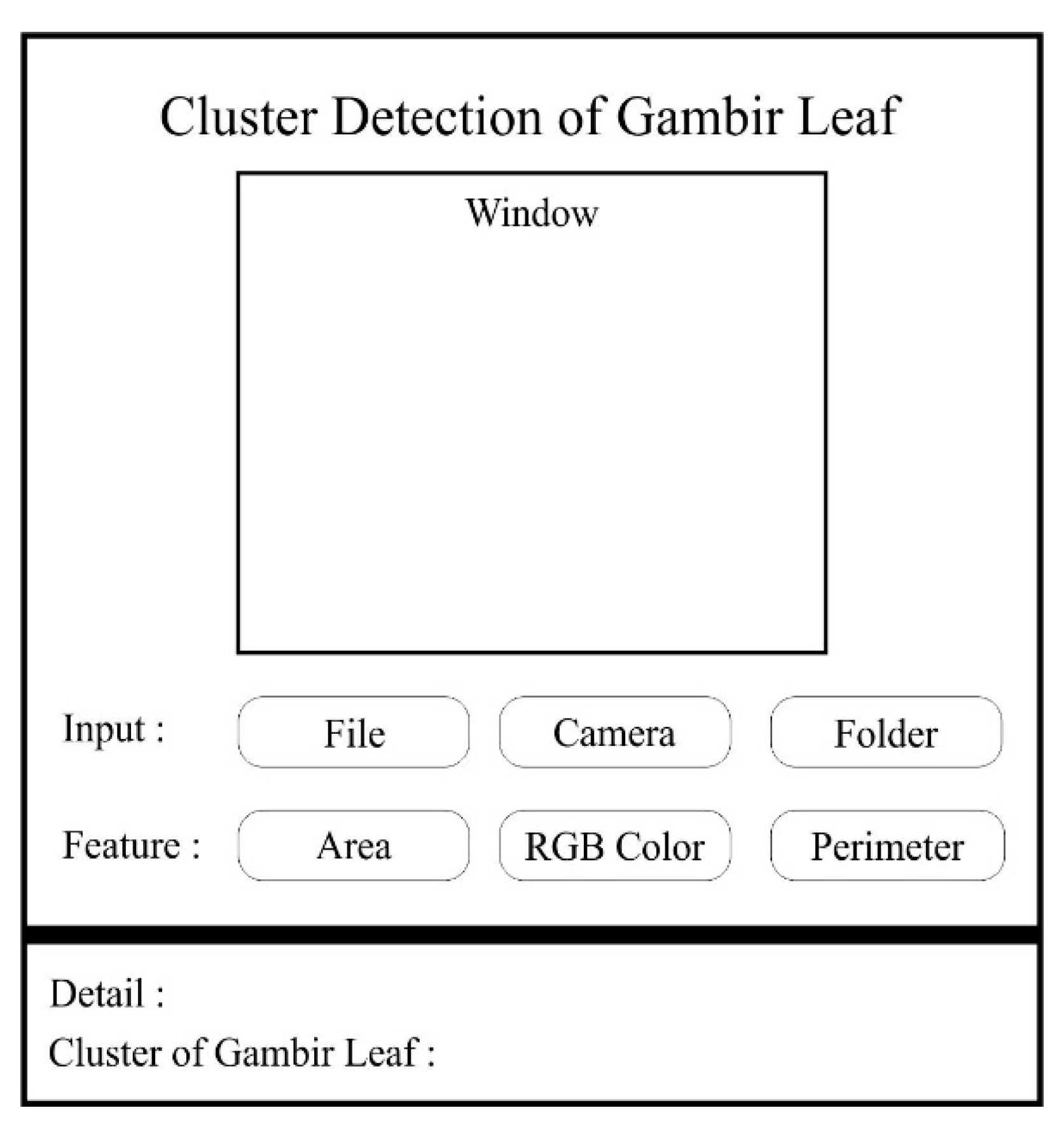
After choosing the input type, the user can choose the feature to predict the grade of leaf. Three features available on the menu are area, perimeter, and color. In particular, the result from a file or camera input type is available in the detail section. This section provides information about area, perimeter, and color. The grade of the leaf is also shown on this part. The layout of this software is illustrated in
Figure 5.
3.3. Leaf Features
Leaf features used in this research were area, perimeter, and intensity of the leaf image. The image was produced by a camera installed at the top side of cover box. The image was represented as a bitmap image in jpeg format, which had pixels. The three features were processed from the image pixels. Captured images were saved in Raspberry Pi memory.
Area
The original image is processed using the grayscale method provided by OpenCV. The RGB value is converted to grayscale using Equation (1). After the gray scale image is obtained, the next step is to get the binary image using threshold Equation (2). The threshold value (T) is set to 70. Pixels are labelled “0” for white if the grayscale value is smaller than threshold and “1” for black if the grayscale is equal or bigger than threshold value. The image is divided into two parts, as follows: Area 1 and 2, as shown by
Figure 6a,b. Each part has a size of 720 pixels × 240 pixels. The leaf area is calculated using horizontal integral projection for both parts, based on Equation (3) for area 1 and Equation (4) for area 2. The total area for the leaf in the pixel is given by Equation (5).
The surface area of the leaf is also measured manually for the validation method, as shown in
Figure 7. The outline of the leaf is projected on millimeter grid paper. The size of the major square on the paper is 1 cm
2. There are two types of filled squares, as follows: Full grid
and half grid
. The total of area
in cm
2 is the sum of full grid and half grid, as in Equation (6). The full grid total is equal to the amount of full squares
(7) and the half grid total is the total of the half grid squares divided by two
(Equation (8)).
Perimeter
The Canny method provided by the cv.Canny() function in OpenCV is used to detect the edges of the leaf image. Hysteresis thresholds were declared to be 70 and 150 for minimum and maximum values, respectively. This method converts the original image into a binary image as shown in
Figure 8. The black pixels are labeled as “0” and white pixels are “1”. Similar to the area procedure, the image is also divided into area 1 and area 2 to calculate the perimeter 1 (Equation (9)) and 2 (Equation (10)), respectively. The total leaf perimeter in the pixel is given by Equation (11).
C1 = perimeter 1 in pixel
C2 = perimeter 2 in pixel
Cp = perimeter of leaf in pixel
P (i, j) = Pixel label in line i and column j.
The perimeter of the leaf is also manually measured to validate the Canny method. The leaf is projected to a millimeter grid paper. Then, a string is attached to trace the line on that paper, as shown by
Figure 9a,b. The length of string is measured using a ruler. The perimeter of the leaf is equal to the length of the string.
Intensity
Image intensity is used to recognize leaf grade. The intensity of the image is calculated using Equation (12). Ten pixels are used as samples for the intensity feature. The coordinates of the ten pixels are set from the lengths and widths of leaves from all grades.
Figure 10 shows the ten sample pixels for the image intensity. There are five areas to position them. Each area has two sample pixels. The horizontal line boundaries located on the camera are vertical pixel 230 for Y
low and vertical pixel 260 for Y
high. The vertical line boundaries are constructed using the horizontal pixel values. Only leaves on grade 5 had ten sample pixels on the leaf. For grade 1, there two sample pixels are located on the leaf and the remaining eight pixels are attached on the background of the image. The completed information about the area vertical boundaries and distribution of the sample locations are provided in
Table 2.
3.4. Neural Network
Each feature has its own artificial neural network (ANN) system. There is an input layer (X
i), one hidden layer (Z
j), and an output layer (Y
k). The hidden and output layer have bias functions b
Zj and b
Yk, respectively. The input layer and the hidden layer is connected with weight (c
ij). The hidden layer and output is weighted by d
jk. The Logsigmoid function is used for the hidden layer and purelin is the activation function for the output layer. The illustration of the ANN is shown by
Figure 11. The output from the hidden layer is calculated using Equation (13) and activated by Equation (14). The output layer produces Equation (15) and is activated by Equation (16).
The number of neurons for each layer is shown by
Table 3. The area and perimeter features, respectively, have two ANN inputs. The area feature uses area 1 and area 2 as the input and the perimeter feature utilizes perimeter 1 and perimeter 2 as the input. The intensity feature uses ten inputs, which are the ten sample pixels. Three binary output neurons as the representatives of the amount of cluster are selected for the output layer. The relationship between the output condition and the grade is shown by
Table 4.
There were 1000 training data sets used to build neuron weight and bias. There were 500 data sets for test sessions. Each grade had 100 data sets to test. The ANN was trained using MATLAB Software to get the weight and bias. The performance of the trained ANN was evaluated based on the accuracy.
5. Conclusions
Gambier leaves in Tarantang village were classified based on farmers’ knowledge into three class; namely, recommended, available, and forbidden to be picked. Five-month-old gambier leaves are recommended to be picked and four-month-old gambier leaf are available to be picked. Younger gambier leaves are forbidden to be picked. Farmers’ ability to classify the gambier leaf were reproduced using three artificial neural networks for each feature of area, perimeter, and intensity. The results show that the neural network with the intensity input was the most accurate system, with a 97% accuracy. The area and perimeter features resulted in 93% and 96% accuracy, respectively. Based on that performance, a set of grading rules was determined using the combination of three neural networks. The recommended class is only given to leaf with an intensity grade of 5 and other features have grade ≥ 4. The leaf is forbidden to be picked if the intensity grade is lower than 5. Those rules can give 100% accuracy to cluster gambier leaves, compared with farmers’ knowledge in this village.


