Article

ParaLarPD: Parallel FPGA Router Using Primal-Dual Sub-Gradient Method

1
Computational Science and Engineering Laboratory, Indian Institute of Technology Indore, Indore 453552, India
2
Electrical and Computer Engineering, National University of Singapore, Singapore 117583, Singapore
3
Center for Advancing Electronics, Technische Universität Dresden, 01062 Dresden, Germany
*
Author to whom correspondence should be addressed.
Electronics 2019, 8(12), 1439; https://doi.org/10.3390/electronics8121439
Submission received: 25 September 2019 / Revised: 25 November 2019 / Accepted: 27 November 2019 / Published: 1 December 2019
(This article belongs to the Section Circuit and Signal Processing)

Abstract

:
In the field programmable gate array (FPGA) design flow, one of the most time-consuming steps is the routing of nets. Therefore, there is a need to accelerate it. In a recent work by Hoo et al., the authors have developed a linear programming (LP)-based framework that parallelizes this routing process to achieve significant speed-ups (the resulting algorithm is termed as ParaLaR). However, this approach has certain weaknesses. Namely, the constraints violation by the solution and a standard routing metric could be improved. We address these two issues here. In this paper, we use the LP framework of ParaLaR and solve it using the primal–dual sub-gradient method that better exploits the problem properties. We also propose a better way to update the size of the step taken by this iterative algorithm. We call our algorithm as ParaLarPD. We perform experiments on a set of standard benchmarks, where we show that our algorithm outperforms not just ParaLaR but the standard existing algorithm VPR as well. We perform experiments with two different configurations. We achieve 20 % average improvement in the constraints violation and the standard metric of the minimum channel width (both of which are related) when compared with ParaLaR. When compared to VPR, we get average improvements of 28 % in the minimum channel width (there is no constraints violation in VPR). We obtain the same value for the total wire length as by ParaLaR, which is 49 % better on an average than that obtained by VPR. This is the original metric to be minimized, for which ParaLaR was proposed. Next, we look at the third and easily measurable metric of critical path delay. On an average, ParaLarPD gives 2 % larger critical path delay than ParaLaR and 3 % better than VPR. We achieve maximum relative speed-ups of up to seven times when running a parallel version of our algorithm using eight threads as compared to the sequential implementation. These speed-ups are similar to those as obtained by ParaLaR.

1. Introduction

According to the Moore’s law, the number of transistors in an integrated circuit is doubling approximately every two years. In the field programmable gate array (FPGA) [1,2] design flow, the routing of nets (which are a collection of two or more interconnected components) is one of the most time-consuming steps. Hence, there is a need to develop fast routing algorithms that tackle the problem of the increasing numbers of transistors per chip, and subsequently, the increased runtime of FPGA CAD (computer-aided design) tools. This can be achieved in two ways. First, by parallelizing the routing algorithms for hardware having multiple cores. However, the pathfinder algorithm [3], which is one of the most commonly used FPGA routing algorithm is intrinsically sequential. Hence, this approach seems inappropriate for parallelizing all types of FPGA routing algorithms.
Second, instead of compiling the entire design together, the users can partition their design, compile partitions progressively, and then assemble all the partitions to form the entire design. Some existing works have proposed this approach [4,5]. However, the routing resources required by one partition may be held by another partition, i.e., there is no guarantee to have balanced partitions. In other words, in this approach, there is a need to tackle the difficulties arising in sharing of routing resources.
The authors in ParaLaR [6] overcome the limitations of existing approaches by formulating the FPGA routing problem as an optimization problem [7]. Here, the objective function is linear and the decision variables can only have binary values. Hence, the FPGA routing problem is converted to a binary integer linear programming (BILP) minimization problem [8,9,10] (generally termed as linear programming (LP)). In this LP, the dependencies (or constraints) that prevent the nets from being routed in parallel are examined and relaxed by using Lagrange relaxation multipliers [11]. The relaxed LP is solved in a parallel manner by the sub-gradient method and the Steiner tree algorithm. The complete algorithm is called ParaLaR.
This parallelization gives significant speed-ups. However, in this approach, the sub-gradient method is used in a standard way that does not always give a feasible solution (i.e., some constraints are violated). This directly impacts the standard metric of minimum channel width, which could also be improved.
There are many variants of the sub-gradient method and a problem-specific method gives better results. In this paper, we use the same framework as for ParaLaR, but use an adapted sub-gradient method. We use a primal–dual variant of the sub-gradient method with an adapted step size in this iterative method. Our approach substantially solves the above two problems.
By experiments on standard benchmarks, we compared our algorithm (termed as ParaLarPD) both with ParaLaR and the commonly used non-parallelizable routing algorithm VPR (Versatile Place and Route) [12]. We performed 100 independent experiments/runs (for all benchmarks) for both ParaLarPD and ParaLaR, and obtained the aggregate results. We performed these experiments for two configurations. For our best configuration, we got results as below. The number of infeasible solutions and the minimum channel width requirement on average reduced by 20 % as compared to ParaLaR (as above, the two metrics are related). Our minimum channel width wa on average 28 % better than that obtained by VPR (there are no constraints that could be violated in VPR). When looking at the total wire length, we obtained the same value as by ParaLaR, which was on an average 49 % better than as obtained by VPR. This is the original metric to be minimized, for which ParaLaR was proposed.
In achieving the above improvements, on an average, the critical path delay in ParaLarPD was 2 % worse than that in ParaLaR and 3 % better than that in VPR. When running a parallel version of ParaLarPD with eight threads, we obtained maximum relative speed-ups of up to seven times over ParaLarPD’s sequential implementation. These speed-ups are similar to those as obtained when comparing parallel ParaLaR and sequential ParaLaR.
There have been some other attempts to improve the performance of VPR in the past few years. Two of the resulting algorithms are RVPack [13] and GGAPack/GGAPack2 [13]. Although these algorithms do not attempt to parallelize the routing process, for the completeness we compare our algorithm to these as well. The rest of this paper is organized as follows: Section 2 describes the formulation of the FPGA routing as an optimization problem. Section 3 explains the implementation of our proposed approach. Section 4 presents experimental results. Finally, Section 5 gives conclusions and discusses future work.

2. Formulation of the Optimization Problem

The routing problem in FPGA or electronic circuit design is a standard problem that is formulated as a weighted grid graph G ( V , E ) of certain set of vertices V and edges E, where a cost is associated with each edge. In this grid graph, there are three types of vertices; the net vertices, the Steiner vertices, and the other vertices. A net is represented as a set N V consisting of all net vertices. A Steiner vertex is not part of the net vertices but it is used to construct the net tree, which is the route of a net (i.e., a sub-tree T of the graph G). A net tree is also called a Steiner tree.
Figure 1 shows an example of a 4 × 4 grid graph, where the black color circles represent the net vertices; the gray color circles represent the Steiner vertices; and the white color circles are the other vertices. The horizontal and the vertical lines represent the edges (as above, these edges have a cost associated with them but that is not marked here). Two net trees are shown by dotted edges.
The number of nets and the set of vertices belonging to each net is given. The objective here is to find a route for each net such that the union of all the routes will minimize the total wire length of the graph G (which is directly proportional to the total path cost). The goal here is to also minimize the channel width requirement of each edge. Both these objectives are explained in detail below, after (1).
To achieve the above two objectives, the problem of routing of nets is formulated as an LP problem given as follows [6] (ParaLaR paper):
min x e , i i = 1 N n e t s e E w e x e , i ,
Subject to i = 1 N n e t s x e , i W , e E ,
A i x i = b i , i = 1 , 2 , . . . , N n e t s and
x e , i = 0 o r 1 .
This optimization problem minimizes the total wire length of FPGA routing, where N n e t s is the number of nets; E is the set of edges with e denoting one such edge; w e is the cost/time delay associated with the edge e; x e , i is the decision variable that indicates whether an edge e (routing channel) is utilized by the net i (value 1) or not (value 0); W is a constant; x i is the vector of all x e , i for net i that represents the ith net’s route tree; A i is the node-arch incidence matrix (which represents a graph as a constraint matrix of the minimum cost flow problem); and b i is the demand/supply vector (which signifies the amount of cost flow to each node).
The inequality constraints are the channel width constraints that restrict the number of nets utilizing an edge to W (which is iteratively reduced; discussed later). The equality constraints guarantee that a valid route tree is formed for each net (these are implicitly satisfied by our solution approach; again discussed later). To find a feasible route for each net efficiently, the above LP should be parallelized. There are two main challenges here, which are discussed in the two sub-sections below.
We use the same elements as used in ParaLaR [6], since we improve that existing algorithm. These elements are discussed in the subsequent paragraphs. There is a slight change of notations, which we have done to make the exposition of our new algorithm more easier. This change of notations is summarized below.
  • Number of nets: N in ParaLaR and N n e t s in ParaLarPD.
  • Cost/time delay associated to edge e: c e in ParaLaR and w e in ParaLarPD.
  • Node–arch incidence matrix: N i in ParaLaR and A i in ParaLarPD.

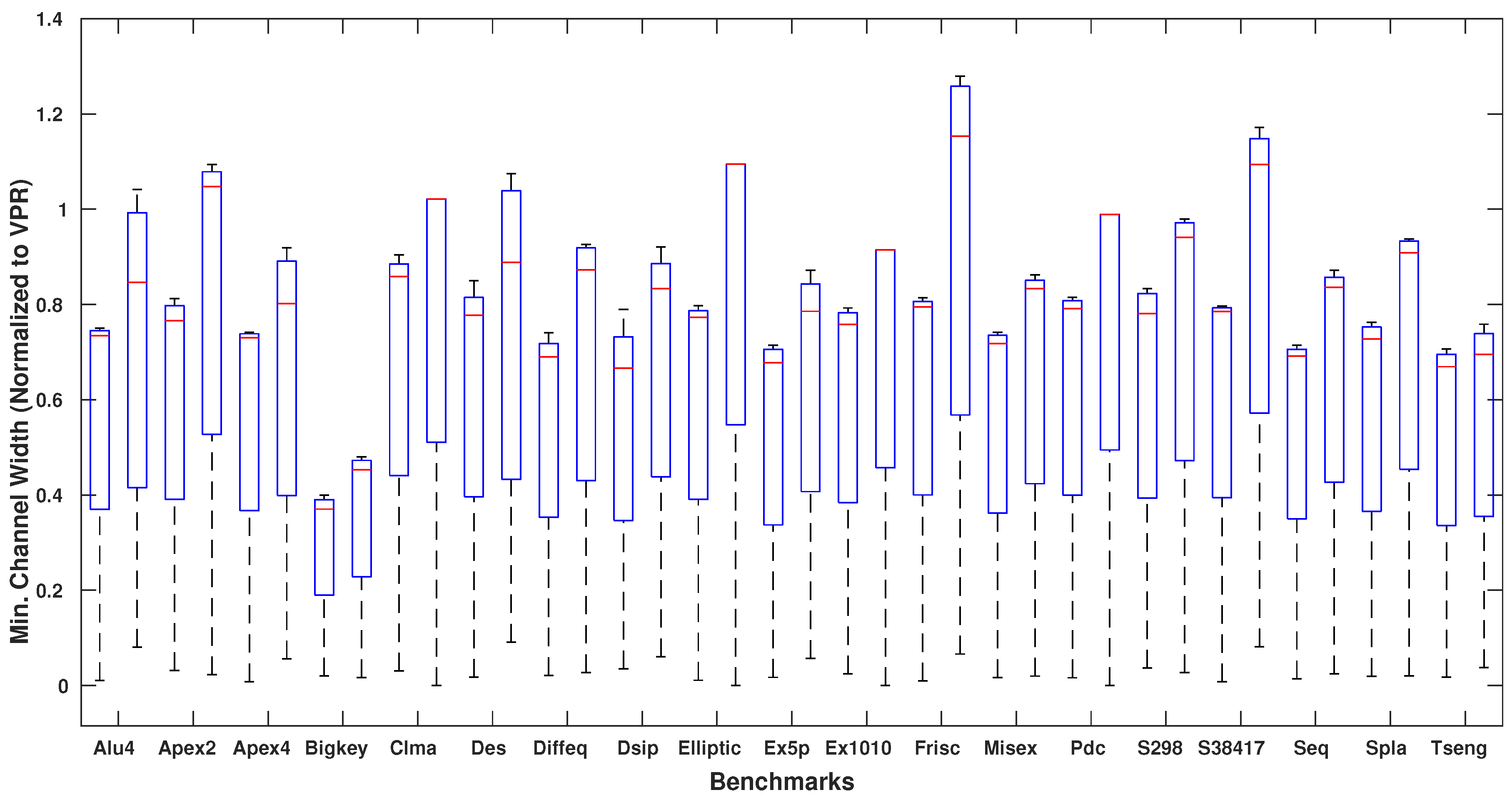
2.1. The Channel Width Constraints

The first challenge to parallelize the LP given in (1)–(2c) is created by the channel width constraints. These constraints introduce dependency in the parallelizing process, and therefore, should be eliminated or relaxed. The Lagrange relaxation [11] is a technique well suited for problems where the constraints can be relaxed by incorporating them into an objective function. If this is not possible, then a Lagrange heuristic can be developed [14,15,16].
In our ParaLarPD, similar to ParaLaR, we introduce Lagrange relaxation multipliers λ e for each channel width constraint (2a), and cumulatively these multipliers represent the cost that prevents overuse of the routing channel. The relaxation of constraints is implemented by adding λ e times the corresponding constraint into the objective function. That is, rewriting (1)–(2c) as in ParaLaR.
min x e , i , λ e i = 1 N n e t s e E w e x e , i + e E λ e i = 1 N n e t s x e , i W ,
Subject to A i x i = b i , i = 1 , 2 , . . . , N n e t s ,
x e , i = 0 o r 1 and
λ e 0 .
After rearranging the objective function above, the modified LP is given as [6]
min x e , i , λ e i = 1 N n e t s e E w e + λ e x e , i W e E λ e ,
Subject to A i x i = b i , i = 1 , 2 , . . . , N n e t s ,
x e , i = 0 o r 1 and
λ e 0 .
In the above LP, w e + λ e is the new cost associated with the edge e. This LP can be easily solved in parallel manner.

2.2. The Choice of Decision Variable

The second challenge to solve the LP given by (5)–(6c) is created by the decision variables x e , i . As earlier, if an edge e is utilized by the net i, then x e , i = 1 else x e , i = 0 . Thus, as mentioned earlier this is a BILP that is non-differentiable, and hence, cannot be solved by conventional methods such as the simplex method [8,17], the interior point method [18], etc. Some methods to solve non-differentiable optimization problems include the sub-gradient-based methods [19], the approximation method [20], etc.
The sub-gradient based methods are commonly used to minimize non-differentiable convex functions f ( x ) . These are iterative in nature that update the variable x as x k + 1 = x k α k g k , where α k and g k are the step size and a sub-gradient of the objective function, respectively, at the kth iteration. In ParaLaR, the LP given in (5)–(6c) is not solved directly by a sub-gradient based method but only the Lagrange relaxation multipliers are obtained by it. After this, the minimum Steiner tree algorithm is used in a parallel manner for FPGA routing. This two-step procedure is followed because just using a sub-gradient method will not always give binary solutions, which we need (recall x e , i can be 0 or 1). Moreover, using a Steiner tree algorithm helps us in achieving feasible routing (equality constraints are implicitly satisfied). In our ParaLarPD, we follow this same approach.

3. Proposed Approach

There are many variants of the sub-gradient based methods such as the projected sub-gradient method [19], the primal–dual sub-gradient method [21], the conditional sub-gradient method [22], the deflected sub-gradient method [22], etc. In ParaLaR [6], authors use the projected sub-gradient method, where the Lagrange relaxation multipliers are calculated as
λ k + 1 = max 0 , λ k + α k h .
Here, λ k and λ k + 1 are the Lagrange relaxation multipliers at the kth and the ( k + 1 ) th iteration, respectively; and h g k , i.e., a sub-gradient of the objective function given in (5) at the kth iteration. Also, as above, α k denotes the size of the step taken in the direction of the sub-gradient at the kth iterative step, and is updated as
α k = 0 . 01 / k + 1 .
This approach satisfactorily parallelizes FPGA routing and gives better results over VPR [12], but there are many inequality constraints that are violated for some cases. This directly affects the minimum channel width requirement, which can be improved further. The channel width is defined as i = 1 N n e t s x e , i .
The LP given by (5)–(6c) is the dual of LP given by (1)–(2c) (see [9,22]). Hence, a sub-gradient method that is specific to a dual problem would give better results compared to the standard one, that is, the primal–dual sub-gradient method. Thus, we use this method with ParaLaR leading to our ParaLarPD. This achieves our main goal of reducing violation of constraints with an added benefit of minimization of channel width.
Next, we describe our ParaLarPD where we compare our usage of primal–dual sub-gradient method with the projected sub-gradient as used in ParaLaR, and also briefly summarized above. As earlier, we expand upon two aspects; iterative update of the Lagrange multipliers and the corresponding step sizes.

Our Algorithm

We update the Lagrange relaxation multipliers in (5)–(6c) as follows [21]
λ e k + 1 = λ e k + α k max 0 , i = 1 N n e t s x e , i W ,
where i = 1 N x e , i W is a sub-gradient of the objective function at the kth iteration—the partial derivative of the objective function in (5) (the h in the projected sub-gradient method from (7) is the same). Also, we take λ e 0 = 0 e E , which is the most general initial guess [11].
Let us now compare (9) with (7). For both the methods, if the inequality constraints are violated at the kth iteration (see (2a); i = 1 N n e t s x e , i W > 0 for some e E ), then the particular Lagrange relaxation multiplier at the ( k + 1 ) th iteration is incremented by α k times the sub-gradient of the objective function at the kth iteration. For the primal–dual sub-gradient method, this is obvious from (9). For the projected sub-gradient method, this is true because λ k is non-negative, and α k and h both are positive in (7).
Further, if the inequality constraints are not violated at the kth iteration (again see (2a); i = 1 N n e t s x e , i W 0 for some e E ), then for the primal–dual sub-gradient method, the value of the particular Lagrange relaxation multiplier at the ( k + 1 ) th iteration is the same as the kth iteration, while for the projected sub-gradient method, it may change (again see (9) and (7), respectively). In general, this works better because logically a Lagrange relaxation multiplier at the ( k + 1 ) th iteration should be equal to the value of this multiplier at the iteration when the particular (or corresponding) constraint is not violated.
Next, we discuss the choice of the step size. If the step size is too small, then the algorithm would get stuck at the current point, and if it is too large, the algorithm may oscillate between any two non-optimal solutions. Hence, it is very important to select the step size appropriately. The choice of step size can be either constant in all the iterations or can be reduced in each successive iteration. In our proposed scheme, the computation of step size involves a combination of the iteration number as well as the norm of the Karush–Kuhn–Tucker (KKT) operator of the objective function at that particular iteration [22] (instead of using the iteration number only, as used in ParaLaR; see (8)). This ensures that the problem characteristic is used in the computation of the step size. That is,
α k = 1 / k / T k 2 ,
where k is the iteration number, T k is the KKT operator for the objective function (5), and T k 2 is the 2-norm of T k .
The sub-gradient based methods are iterative algorithms, and hence, we need to check when to stop. There is no ideal stopping criterion for sub-gradient based methods. However, some possible measures that can be used are discussed below (including our choice) [19].
  • If at an iteration k, the constraints violation (2a) (i.e., g k 0 ) is satisfied and λ k g k = 0 , then we obtain the optimal point. Therefore, we stop here because there is no constraint violation (a necessary condition of Lagrange relaxation) [11]. However, this stopping criterion is achieved only if strong duality holds but, in case of our problem, there is weak duality. Details of strong and weak duality can be found in [9,22].
  • Let at iteration k, f * and f k be the optimal function value and the available function value at the kth iteration, respectively, then the sub-gradient iterations can be stopped when | f k f * | ϵ (where ϵ is a very small positive number). In this criterion, the optimal value of the objective function is required in advance, which we do not have.
  • Another approach is to stop when the step size becomes too small. This is, because the sub-gradient method would get stuck at the current iteration.
As none of the above stopping criteria fit us, we stop our algorithm after a sufficient and a fixed number of iterations, as used in ParaLaR. As earlier, we term our proposed algorithm as ParaLarPD because we use primal–dual sub-gradient algorithm with ParaLaR.
Rest of steps of our ParaLarPD are the same as in ParaLar. We start with a constant value of W and solve the optimization problem (5)–(6c) by combination of the sub-gradient method and the Steiner tree algorithm. This gives us the total wire length and the constraint violation (or channel width).
Next, we reduce the value of W and again follow the above steps to obtain better local minima both for the total wire length and the constraint violation (or channel width).
The pseudocode of our ParaLarPD is given in Algorithm 1, where the new addition to ParaLaR are captured by lines 6 and 16.
Algorithm 1 ParaLarPD
   Input: Architecture description file and benchmark file.
   Output: Route edges.
 1:
Run VPR with the input architecture and benchmark circuit.
 2:
s t e i n e r _ p o i n t s Ø                ▹ Initialize Steiner points
 3:
g r i d _ g r a p h InitGridGraph()                 ▹ Initialize grid graph
 4:
λ e = 0 , e E             ▹ Initialize Lagrangian relaxation multipliers
 5:
for   i t e r = 1   to   m a x _ i t e r   do
 6:
     Calculate the step size α using the Equation (10).                ▹ It is used to update λ e
 7:
      r o u t e _ e d g e s Ø
 8:
     parallel_for i = 1   to N n e t s do               ▹ N n e t s number of nets
 9:
           p o i n t s p : p { source   and   sink   of   i th   net }
10:
         if i t e r = = 1 then
11:
                s t e i n e r _ p o i n t s [ i th n e t ] MST( g r i d _ g r a p h , p o i n t s )        ▹ MST is call to a function that executes a Minimum Steiner Tree.
12:
        end if
13:
         r o u t e _ e d g e s [ i th n e t ] MST( g r i d _ g r a p h , s t e i n e r _ p o i n t s [ i th n e t ] p o i n t s )
14:
   end parallel_for
15:
   while e E do
16:
        Update Lagrangian relaxation multipliers λ e using the Equation (9).
17:
        Update the edge weight of the g r i d _ g r a p h on r o u t e _ e d g e . New edge weights are w e + λ e
18:
  end while
19:
end for
In the above algorithm, initially we pack and place the benchmark circuit using VPR (as described in the architecture file). Next, set of Steiner points are initialized as empty, the grid graph is initialized to model an FPGA that is large enough to realize the input netlist ( N n e t s is the number of total nets), and the Lagrangian relaxation multipliers (i.e.,  λ e ) are initialized to zero. Next, the routing algorithm runs for m a x _ i t e r (which is set to 50) number of iterations. In each iteration, first, we calculate the step size. Thereafter, we initialize r o u t e _ e d g e s as empty set. Then, the for loop at line 8 routes the nets in parallel by running the minimum Steiner tree (MST) algorithm to obtain the route edges. Finally, edge weights of the g r i d _ g r a p h are updated in the while loop from line 15 to line 18. In Appendix A, we have listed a code snippet, which is the actual code of important functions.

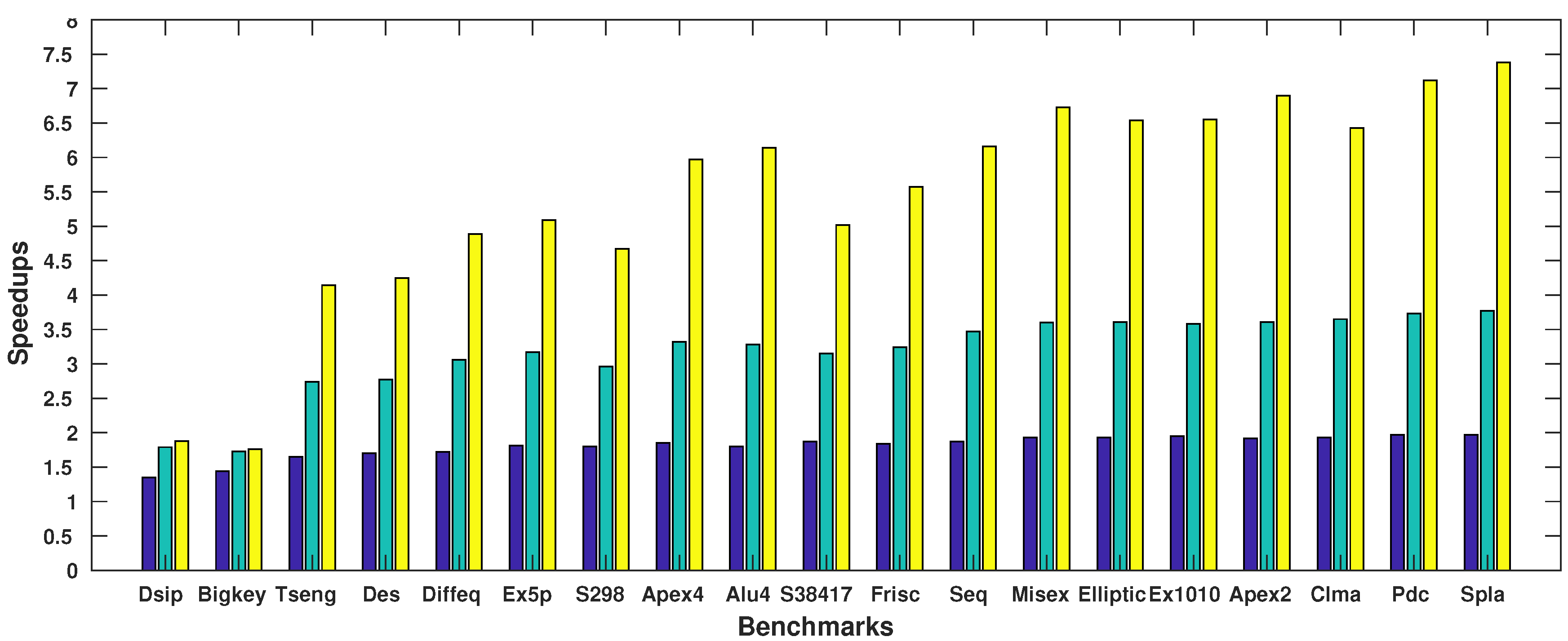
4. Experimental Results

We performed experiments on a machine with single Intel(R) Xeon(R) CPU E5-1620 v3 running at 3.5 GHz and 64 GB of RAM. The operating system was Ubuntu 14.04 LTS, and the kernel version is 3.13.0–100. Our code was written in C++11 and compiled using GCC version 4.8.4 with O3 optimization flag. The resulting compiled code was run using a different number of threads.
We compared our proposed ParaLarPD with ParaLaR [6] and VPR [12]. For comparison purposes, ParaLaR and VPR 7.0 from the verilog-to-routing (VTR) package were compiled using the same GCC version and optimization flag.
As discussed earlier, besides ParaLaR and VPR, other commonly used routing algorithms are random VPack (RVPack) [13] and grouping genetic algorithm pack (GGAPack/GGAPack2) [13]. We discuss the benefits of ParaLarPD over these two algorithms as well.
The architecture parameters used for our experiments are given in Table 1, which are most commonly used [12,13,23].
In Table 1, the values of N and K specify that the CLBs in the architecture contained ten fracturable logic elements (FLEs) and each FLE had six inputs, respectively. The values of F c i n and F c o u t specify that every input and output pin was driven by 15% and 10%, of the tracks in a channel, respectively. We also performed experiments with F c i n = 1 and F c o u t = 1 , the results of which are not reported in this paper. However, our algorithm still gave better results than ParaLaR and VPR. In FPGA terminology, the value of F s specifies the number of wire segments that can be connected to each wire segment where horizontal and vertical channels intersect. This value can only be a multiple of 3. Here, we performed experiments with F s = { 3 , 6 } . The value of length specifies the number of logic blocks spanned by each segment. We took this as 4, although our proposed method can be used for architectures with varying lengths, e.g., length = 1 or a mix of length = 1 and length = 4 . All these parameters (i.e., N, K, F c i n , F c o u t , F s , and length) in ParaLaR and VPR were modified according to the values given in Table 1, to run them identical to our model.
We tested on MCNC benchmark circuits [24], which ranged from small sized to large sized logic blocks. Initially, the circuits were packed and placed using VPR. After that, routing was performed by all three methods (i.e., our proposed ParaLarPD, ParaLaR, and VPR). For parallelization, we used Intel threading building blocks (TBB) libraries. To examine the behavior of ParaLarPD and ParaLaR, we performed 100 independent runs of each of ParaLarPD and ParaLaR (for all benchmarks) and then collected the aggregate results of these 100 runs.
There is no general rule of choosing the initial value of the channel width for experimental purposes. However, a value of 20 % to 40 % more than the minimum channel width obtained from VPR is commonly used [6,23]. For our experiments, both ParaLarPD and ParaLaR are initialized with initial channel width (W) as 1.2 W m i n , where W m i n is the minimum channel width obtained from VPR. We also do experiments with initial W as 1.4 W m i n , which does not change the results. We use an upper limit of 50 for the number of iterations for all the three methods because this is the limit chosen in the experiments of ParaLaR from [6]. The best results out of all these iterations are reported.
Also, in our proposed model, routing of individual nets is independent and we update the cost of utilizing the edges at the end of each routing iteration. Thus, there is no race condition leading to no randomness. Hence, our executions are deterministic.
In Table 2 and Table 3, we compare the channel width (also called the minimum channel width), the total wire length, and the critical path delay as obtained by our proposed ParaLarPD with ParaLaR and routing-driven VPR. These metrics are independent of the number of threads used, therefore, here we give results for a single thread only. The results of ParaLarPD and ParaLaR are the average values of their 100 independent runs. In the tables, we report the geometric mean (Geo. Mean) of all the values obtained for different benchmark circuits. It indicates the central tendency of a set of numbers and is commonly used [6].
It is important to emphasize that ParaLaR is sensitive to the system configuration of the machine used for experiments (in fact, ParaLarPD is equally sensitive). Hence, the ParaLaR data in Table 2 and Table 3 is slightly different than that reported in the original ParaLaR paper.
In Table 2 (i.e., for F s = 3 ), if we look at the channel width, then ParaLarPD gives on an average 20.16 % improvement over ParaLaR. As discussed earlier, constraints violation (which is a problem in ParaLaR) is directly related to the minimum channel width. Hence, ParaLarPD proportionally improves the constraints violation of ParaLaR. Further, ParaLarPD gives on an average 27.71 % improvement in the channel width when compared with VPR (in VPR, there is no concept of constraints violation). If we look at the total wire length, then ParaLarPD achieves the same value as obtained by ParaLaR, which is on an average 48.86 % better than the one obtained by VPR.
While the focus of this work is minimizing the maximum channel width, we did measure the impact of the algorithm on the critical path delay. The average critical path delay of ParaLarPD is 1.52 % worse as compared to ParaLaR and 2.55 % better as compared to VPR. Considering the significant improvements in minimum channel width, i.e., 20.16%, and almost the same speed-up (when compared to ParaLaR), we believe this trade-off is still reasonable since the critical path delay is not deteriorated significantly.
Similarly, in Table 3 (i.e., for F s = 6 ), if we look at the channel width, then ParaLarPD gives on an average 18.47 % improvement over ParaLaR (as above, this gives the same improvement in the constraints violation). The improvement in comparison to VPR is on average 22.01%. If we look at the total wire length, then ParaLarPD achieves the same value as obtained by ParaLaR, which is on an average 45.61 % better than the one obtained by VPR. Similar to Table 2, the critical path delay obtained by using ParaLarPD is only slightly worse than ParaLaR and VPR; about 4.76 % worse than ParaLaR and 6.36 % worse than VPR.
To better demonstrate the improvements of ParaLarPD over ParaLaR, we compare them on an average and in percentage terms separately in Table 4. In this table, we give percentage improvement of ParaLarPD over ParaLaR, where all the results (i.e., the channel width, wire length, and critical path delay) are obtained as the geometric mean of the maximum, minimum, average, and standard values of 100 independent runs for all benchmarks. As above, and also evident from this table, ParaLarPD performs substantially better on channel width and almost the same on total wire length and critical path delay. We see from Table 4 that for F s = 3 , the average standard deviation value of critical path delay of ParaLarPD is 86.9% lower as compared to ParaLaR, while for F s = 6 , ParaLarPD has 111.11% higher critical path delay as compared to ParaLar. However, the standard deviation is just a measure of the amount of variation. It does not imply that ParaLarPD has this much percentage of lower or higher delay.
In addition to above tables, we also represent the maximum, minimum, average, and standard deviation values of the channel width (for all the benchmarks, and when obtaining them for 100 independent runs) of ParaLarPD and ParaLaR [6] (for the configuration F s = 3 , l e n g t h = 4 , F c i n = 0.15 and F c o u t = 0.10 ). This result is shown by the box plot graph, shown in Figure 2. In this figure, all the values are normalized to VPR (given in Table 2). From this figure, we can see that ParaLarPD is always better than VPR, since all values are below 1, even in the worst cases observed in 100 runs. Hence, from the above discussion and this figure, we can see that ParaLarPD performs better than ParaLaR and VPR. We have not included the figures for the wire length and the critical path delay since the values of these metrics are almost the same for both ParaLarPD and ParaLaR.
Recall, the underlying goal of ParaLaR and this work is to efficiently parallelize the routing process. Hence, next we report results when using different number of threads in Table 5. The benchmark dataset used (first column in Table 5) is the same as discussed in the earlier paragraphs.
First, we discuss the speed-ups obtained when using different number of threads for ParaLarPD. The absolute execution time (in seconds) for different threads is given in columns two through five and is represented as 1X, 2X, 4X, and 8X. The relative speed-ups are given in columns six through eight and are calculated as below.
Speedup = Execution time with 1 thread Execution time with n threads .
It can be observed from this data that when we used ParaLarPD with 2 threads, on an average, speed-up of up to 1.80 times was observed (over the single thread execution). Similarly, when using 4 threads and 8 threads, on an average, speed-up of up to 3.11 times and 5.11 times, respectively, was observed (over the single thread execution).
To show the dependency between the size of the benchmark circuits and their speed-ups, we plot a bar graph (Figure 3). In this figure, on the x-axis, we have the benchmark circuits in the increasing order of their execution time when running them with one thread, which is directly proportional to the size of the benchmark circuits [6]. On the y-axis, we have the speed-ups of these benchmark circuits when running them with different threads. We use three different colored bars to represent speed-ups with two threads, four threads, and eight threads. From this figure, it can be observed that for large benchmark circuits, the speed-ups of ParaLarPD nearly match the ideal speed-ups (proportional to the number of threads used). For example, the last circuit or “spla” has speed-ups of 1.97 , 3.77 , and 7.38 , which are very close to their corresponding ideal speed-ups of 2, 4, and 8, respectively.
To compare the speed-up of ParaLarPD and ParaLaR, we perform experiments with the same number of threads for both of them. We obtain almost the same execution times for both, and hence, we do not report this data.
Next, we compare ParaLarPD’s execution time with VPR’s execution time. This data is given in columns nine and ten of Table 5. We can observe from these columns that on an average ParaLarPD (when executed using a single thread) is 2.70 times faster than VPR. Since in VPR, there is no concept of using multiple threads, we could not compare ParaLarPD’s data for a higher number of threads with it. Next, we compare the performance of ParaLarPD with RVPack [13] and GGAPack2 [13] algorithms. We do not perform a direct comparison between our ParaLarPD and these two algorithms. Rather, we use VPR as an intermediate algorithm for comparison. Thus, in Table 6, we give the percentage improvement of ParaLarPD over VPR, and improvement of RVPack and GGAPack2 over VPR. We follow this strategy for two reasons. First, the architecture parameters as used in these two algorithms are different from ours, and using our parameters for executing them and their parameters for executing ParaLarPD would lead to an unfair comparison. Second, these two algorithms have randomness associated with them, and hence, the results are difficult to replicate. As evident from Table 6, ParaLarPD outperforms these two algorithms in-terms of all metrics.

5. Conclusions and Future Work

In this work, we extend the work of [6] (ParaLaR algorithm) in proposing a more effective parallelized FPGA router. We use the LP framework of [6] and use the primal–dual sub-gradient method with a better update of the Lagrange relaxation multipliers and the corresponding step sizes.
Experiments on MCNC benchmark circuits show that for our best configuration ParaLarPD outperforms not just ParaLaR, but VPR too, which is a commonly used standard algorithm for FPGA routing. That is, ParaLarPD gives 20 % average improvement in the standard metric of the minimum channel width and the constraints violation (both of which are related) when compared to ParaLaR. When compared to VPR, we see an average improvement of 28 % in the minimum channel width (in VPR, there is no concept of constraints violation). We obtained the same value for another standard metric of total wire length as obtained by ParaLaR. This is 49 % better on an average than the corresponding data for VPR.
While achieving the above improvements, the critical path delay in ParaLarPD was on average about 2 % worse than that in ParaLaR and about 3 % better than that in VPR. When running ParaLarPD in parallel manner with eight threads, we attained peak relative speed-ups of up to seven times over its sequential execution. These speed-ups are similar to those as obtained when comparing parallel ParaLaR and sequential ParaLaR.
The Lagrange relaxation technique that we use is not always guaranteed to satisfy the corresponding constraints (as observed in Section 3 and Section 4). Hence, one future direction is to develop a Lagrange heuristic [14,15,16] specific to our problem to avoid this behavior. Another future direction involves finding more efficient algorithms for solving this BILP, which we know is an NP-complete problem.

Author Contributions

Investigation, R.A.; writing—original draft, R.A. and K.A.; supervision, K.A.; formal analysis, C.H.H.; software, T.D.A.N.; project administration, A.K.

Funding

This research received no external funding.

Conflicts of Interest

The authors declare no conflict of interest.

Appendix A. Code Snippet of ParaLarPD

Including complete code will take lot of space and increase the length of paper. So, instead of this, we give code snippet of our ParaLarPD. It highlights the Steiner tree part of our ParaLarPD, and provides only the definition of other functions, which are self-explanatory. Other components of this code are given in the comment sections within the code, which are also self-explanatory.
# include " pch . hpp"
# include " router . hpp"
# include " netlist . hpp"
# include " mst . hpp"
# include " timing . hpp"
# include <cmath>
GridGraph create_grid_graph ( int nx , int ny )
{
// Create a grid graph .
}
extern int MAX_ITER;
void Router : : parallel_route_tbb_new_netlist ( Netlist &netlist , int num_threads )
{
        Mst<GridGraph> mst ;
        int max_iter = MAX_ITER;
        boost : : timer : : nanosecond_type total _ routing_ time = 0 ;
        for ( const auto &e : grid . edges ( ) ) {
// Initialization of varialbes .
        }
        vector <Net> nets ;
        nets . reserve ( netlist . nets . size ( ) ) ;
        int temp = 0 ;
        for ( const auto &net : netlist . nets ) {
                 Net temp_net ;
                 temp_net . index = temp++;
                 temp_net . name = net . second−>name ;
                 temp_net . points . emplace_back ( net . second−>source−>port−>block−>position ) ;
                 for (const auto &sink : net . second−>s inks ) {
                          temp_net . points . emplace_back ( sink−>port−>block−>pos i t ion ) ;
                 }
                 nets . emplace_back ( std : :move( temp_net ) ) ;
        }
        vector < list <Point >> previous _ steiners ( nets . size ( ) ) ;
        for ( int iter = 0 ; iter < max_iter ; ++ iter ) {
                 for ( const auto &e : grid . edges ( ) ) {
                          GridGraphEdgeObject &obj = get ( edge_object , grid , e ) ;
                          obj . util = 0 ;
                          assert ( obj . delay == 1 ) ;
                          put ( edge_weight , grid , e , obj . delay + obj . mult ) ;
                 }
                 mst . init ( grid ) ;
                 vector < list <GridGraph : : edge_descriptor >> route_edges ( nets . size ( ) ) ;
                 boost : : timer : : cpu_timer timer ;
                 clock_ t iter _ begin = clock ( ) ;
                 timer . start ( ) ;
                 int total _wirelength = 0 ;
                 const bool nested_zel = true ;
                 i f ( iter == 0) {
                           if ( ! nested_zel ) {
                                     int net_num = 0 ;
                           for ( const auto &net : nets ) {
mst . parallel_zel_new_reduce ( grid , net . points , previous _ steiners [ net_num ] ) ;
net_num++;
                          }
                          } else {
tbb : : parallel _ for ( tbb : : blocked_range <int >(0 , nets . size ( ) ) ,
[&mst , &nets , &previous _ steiners , this ]
( const tbb : : blocked_range <int > &range ) −> void
                          {
                          for ( int i = range . begin ( ) ; i != range . end ( ) ; ++i ) {
                                     if ( nets [ i ] . point s . size ( ) <= 70) {
mst . parallel_zel_new_reduce ( grid , nets [ i ] . points , previous _ steiners [ i ] ) ;
                                                }
                                     }
                          } ) ;
                          }
                 }
tbb : : spin_mutex mutex ;
tbb : : parallel _ for ( tbb : : blocked_range <int >(0 , nets . size ( ) ) ,
[&mutex , &route_edges , &total _wirelength , &mst , &nets , &previous _ steiners , this ]
( const tbb : : blocked_range <int > &range ) −> void
                          {
                          for ( int i = range . begin ( ) ; i != range . end ( ) ; ++i ) {
                                     {
                                     tbb : : spin_mutex : : scoped_lock lock (mutex ) ;
                                     total _wirelength += route_edges [ i ] . size ( ) ;
                                     }
                          for ( const auto &e : route_edges [ i ] ) {
                          GridGraphEdgeObject &obj = get ( edge_object , grid , e ) ;
                                     {
                                     tbb : : spin_mutex : : scoped_lock lock (mutex ) ;
                                     obj . util += 1 ; / / channel width
                                     }
                          }
                          }
                          }
                 ) ;
// Calculate 2−norm of the KKT operator of the objective function .
// Update the step size .
                 for ( const auto &e : grid . edges ( ) ) {
// Update Lagrangian relaxation multipliers , channel width and wire length .
                 }
// Do timing analysis ( calculate the critical path delay and the execution time ) .
// Print results of each iteration .
// Update the best results .
        }
// Print the best results at the end of all iterations
}

References

  1. Yu, H.; Lee, H.; Lee, S.; Kim, Y.; Lee, H.M. Recent advances in FPGA reverse engineering. Electronics 2018, 7, 246. [Google Scholar] [CrossRef]
  2. Jiang, Y.; Chen, H.; Yang, X.; Sun, Z.; Quan, W. Design and Implementation of CPU & FPGA Co-Design Tester for SDN Switches. Electronics 2019, 8, 950. [Google Scholar]
  3. McMurchie, L.; Ebeling, C. PathFinder: A negotiation-based performance-driven router for FPGAs. In Proceedings of the 3rd International Symposium on Field-Programmable Gate Arrays, Napa, VA, USA, 12–14 February 1995; pp. 111–117. [Google Scholar]
  4. Cabral, L.A.F.; Aude, J.S.; Maculan, N. TDR: A distributed-memory parallel routing algorithm for FPGAs. In Proceedings of the 12th International Conference on Field-Programmable Logic and Applications (FPL), Montpellier, France, 2–4 September 2002; pp. 263–270. [Google Scholar]
  5. Gort, M.; Anderson, J.H. Accelerating FPGA routing through parallelization and engineering enhancements special section on PAR-CAD 2010. IEEE Trans. Comput. Aided Des. Integr. Circuits Syst. 2012, 31, 61–74. [Google Scholar] [CrossRef]
  6. Hoo, C.H.; Kumar, A.; Ha, Y. ParaLaR: A parallel FPGA router based on Lagrangian relaxation. In Proceedings of the 25th International Conference on Field-Programmable Logic and Applications (FPL), London, UK, 2–4 September 2015; pp. 1–6. [Google Scholar]
  7. Lee, H.; Kim, K. Real-Time Monte Carlo Optimization on FPGA for the Efficient and Reliable Message Chain Structure. Electronics 2019, 8, 866. [Google Scholar] [CrossRef]
  8. Bartels, R.H.; Golub, G.H. The Simplex method of linear programming using LU decomposition. Commun. ACM 1969, 12, 266–268. [Google Scholar] [CrossRef]
  9. Hashemi, S.M.; Modarres, M.; Nasrabadi, E.; Nasrabadi, M.M. Fully fuzzified linear programming, solution and duality. J. Intell. Fuzzy Syst. 2006, 17, 253–261. [Google Scholar]
  10. Ali, H.; Ali, Y.M.; Mashaalah, M. Linear programming with rough interval coefficients. J. Intell. Fuzzy Syst. 2014, 26, 1179–1189. [Google Scholar]
  11. Fisher, M.L. The Lagrangian relaxation method for solving integer programming problems. Manag. Sci. 1981, 27, 1–18. [Google Scholar] [CrossRef]
  12. Betz, V.; Rose, J. VPR: A new packing, placement and routing tool for FPGA research. In Proceedings of the 7th International Workshop on Field-Programmable Logic and Applications (FPL), London, UK, 1–3 September 1997; pp. 213–222. [Google Scholar]
  13. Wang, Y. Circuit Clustering for Cluster-Based FPGAs Using Novel Multiobjective Genetic Algorithms. Ph.D. Thesis, University of York, York, UK, 2015. [Google Scholar]
  14. Czibula, O.G.; Gu, H.; Zinder, Y. A Lagrangian relaxation-based heuristic to solve large extended graph partitioning problems. In WALCOM: Algorithms and Computation; Kaykobad, M., Petreschi, R., Eds.; Lecture Notes in Computer Science 9627; Springer: Cham, Switzerland, 2016; pp. 327–338. [Google Scholar]
  15. Holmberg, K.; Joborn, M.; Melin, K. Lagrangian based heuristics for the multicommodity network flow problem with fixed costs on paths. Eur. J. Oper. Res. 2008, 188, 101–108. [Google Scholar] [CrossRef]
  16. Deleplanque, S.; Sidhoum, S.K.; Quilliot, A. Lagrangean heuristic for a multi-plant lot-sizing problem with transfer and storage capacities. RAIRO-Oper. Res. 2013, 47, 429–443. [Google Scholar] [CrossRef]
  17. Polo-López, L.; Córcoles, J.; Ruiz-Cruz, J. Antenna Design by Means of the Fruit Fly Optimization Algorithm. Electronics 2018, 7, 3. [Google Scholar] [CrossRef]
  18. Lustig, I.J.; Marsten, R.E.; Shanno, D.F. Interior point methods for linear programming: Computational state of the art. ORSA J. Comput. 1994, 6, 1–14. [Google Scholar] [CrossRef] [Green Version]
  19. Boyd, S.; Xiao, L.; Mutapcic, A. Subgradient methods. Notes for EE392o Stanford University. Available online: https://web.stanford.edu/class/ee392o/ (accessed on 24 January 2019).
  20. Bertsekas, D.P. Nondifferentiable optimization via approximation. In Nondifferentiable Optimization; Balinski, M.L., Wolfe, P., Eds.; Mathematical Programming Studies 3; Springer: Berlin/Heidelberg, Germany, 1975; pp. 1–25. [Google Scholar]
  21. Boyd, S. Primal-Dual Subgradient Method. Notes for EE364b Stanford University. Available online: https://stanford.edu/class/ee364b/lectures/ (accessed on 24 January 2019).
  22. Guta, B. Subgradient Optimization Methods in Integer Programming with an Application to a Radiation Therapy Problem. Ph.D. Thesis, Technische Universität Kaiserslautern, Kaiserlautern, Germany, 2003. [Google Scholar]
  23. Moctar, Y.; Stojilović, M.; Brisk, P. Deterministic parallel routing for FPGAs based on Galois parallel execution model. In Proceedings of the 28th International Conference on Field-Programmable Logic and Applications (FPL), Dublin, Ireland, 27–31 August 2018; pp. 21–25. [Google Scholar]
  24. Yang, S. Logic Synthesis and Optimization Benchmarks User Guide: Version 3.0; Microelectronics Center of North Carolina (MCNC): Research Triangle Park, NC, USA, 1991. [Google Scholar]
Figure 1. A 4 × 4 grid graph showing the different type of vertices and routing channels.
Electronics 08 01439 g001
Figure 2. The box plot graph of maximum, minimum, average, and standard deviation values of the channel width obtained by our proposed algorithm (ParaLarPD) and by the algorithm from which we have extended (ParaLaR [6]). All the values are normalized to VPR. This plot graph is for all the benchmarks, and when executing them for 100 independent runs. The left hand side box of each benchmark corresponds to ParaLarPD and the right hand side box of each benchmark corresponds to ParaLaR.
Electronics 08 01439 g002
Figure 3. Speed-ups of each benchmark when running it with two, four, and eight threads. These benchmarks are arranged from left to right in their increasing order of execution time when running them with one thread, which is directly proportional to the size of the benchmark.
Electronics 08 01439 g003
Table 1. FPGA design architecture parameters used in our experiments.
NK F cin F cout F s Length
1060.150.10{3, 6}4
Table 2. Comparison of quality of results, i.e., channel width, total wire length, and critical path delay (in nanoseconds) between our proposed algorithm (ParaLarPD), the algorithm from which we have extended (ParaLaR [6]), and the standard algorithm used for routing (VPR [12]). These results are reported for the configuration parameter F s equal to 3, which signifies the number of wire segments that can be connected to each wire segment where horizontal and vertical channels intersect. The results of ParaLarPD and ParaLaR are the average values of their 100 independent runs (rounded to 2 and 0 decimal places, respectively).
BenchmarkChannel WidthTotal Wire LengthCritical Path Delay (ns)
circuits [24]ParaLarPDParaLaRVPRParaLarPDParaLaRVPRParaLarPDParaLaRVPR
Alu435.5445.27485030502910,4807.307.017.50
Apex250.0768.06647935793415,8817.417.167.26
Apex445.5753.48625630563210,7467.086.736.92
Bigkey19.0323.27503896389670524.014.443.53
Clma 81.4496.009449,27849,28487,39815.4616.3115.08
Des31.1740.10406952695214,7395.545.545.83
Diffeq37.5249.23544349435091405.655.727.09
Dsip25.6332.33384778477897423.623.454.20
Elliptic57.4281.007415,12415,12428,27110.8310.9113.98
Ex5p48.8257.00704889488110,1696.946.287.69
Ex101063.3175.008223,59623,95043,91914.5712.7110.05
Frisc68.71106.388619,48419,48435,66413.1312.8415.38
Misex42.2748.67585194519210,0616.496.686.08
Pdc73.6791.009230,42330,42553,66112.6312.4911.75
S29839.0046.29485250525010,29112.7112.0816.62
S3841750.4872.006421,90721,90642,59710.4310.038.82
Seq48.8559.00707654765314,2036.146.186.09
Spla 59.4174.338020,11720,11737,38410.4310.6910.11
Tseng39.6541.67582484248461485.785.786.75
Geo. Mean45.5557.0562.759041904717,6798.037.918.24
Table 3. Comparison of quality of results, i.e., channel width, total wire length, and critical path delay (in nanoseconds) between our proposed algorithm (ParaLarPD), the algorithm from which we have extended (ParaLaR [6]), and the standard algorithm used for routing (VPR [12]). These results are reported for the configuration parameter F s equal to 6, which signifies the number of wire segments that can be connected to each wire segment where horizontal and vertical channels intersect. The results of ParaLarPD and ParaLaR are the average values of their 100 independent runs (rounded to 2 and 0 decimal places, respectively).
BenchmarkChannel WidthTotal Wire LengthCritical Path Delay (ns)
circuits [24]ParaLarPDParaLaRVPRParaLarPDParaLaRVPRParaLarPDParaLaRVPR
Alu435.7146.11445118511895458.057.596.82
Apex250.8059.62607933793315,6297.407.797.29
Apex445.5064.21585609560710,6207.017.056.94
Bigkey18.5024.75523919391966804.583.923.40
Clma 77.0296.008849,60649,59284,68416.4815.0513.50
Des34.3837.54507010701112,9776.306.306.08
Diffeq38.3052.73504424442691096.446.276.63
Dsip24.4129.65344733473390864.473.954.25
Elliptic57.6978.007015,07215,06927,48310.2610.2011.78
Ex5p46.2557.75624817481590036.816.326.36
Ex101064.5280.007423,01423,01240,99512.8912.4610.75
Frisc67.5082.847819,48319,48734,06512.9713.1814.91
Misex45.4250.56525223522395136.066.275.75
Pdc74.2785.138430,40130,39653,92413.2713.2711.75
S29839.8145.004453305330923712.7010.9910.99
S3841751.3875.876021,94921,95239,83610.999.449.71
Seq55.2358.00647651765013,6207.316.746.75
Spla 60.3871.757420,47120,47136,14611.4011.099.24
Tseng35.7038.73502472247252265.255.256.04
Geo. Mean45.8156.1958.749057905816,6538.367.987.86
Table 4. The percentage improvement of our proposed algorithm (ParaLarPD) over ParaLaR [6] for 100 independent runs. Here, the terms Max., Min., Ave., and STD denote the maximum, minimum, average, and standard deviation values, respectively.
Value of F s Channel WidthTotal Wire LengthCritical Path Delay
Max.Min.Ave.STDMax.Min.Ave.STDMax.Min.Ave.STD
319.9816.720.1652.630.090.030.0720.69 0.86 1.67 1.52 86.9
618.216.4918.4739.730.050.090.011 9 5.9 3.55 4.76 111.11
Table 5. Execution time (in seconds) of our proposed algorithm (ParaLarPD) when running it with multiple threads, its relative speed-ups, and comparison of ParaLarPD’s execution time (when runnig it with one thread) with VPR’s [12] execution time. These results are reported for the configuration parameter F s equal to 3, which signifies the number of wire segments that can be connected to each wire segment where horizontal and vertical channels intersect.
BenchmarkExecution Time of ParaLarPD (s)ParaLarPD’s Speed-UpsComparison with VPR
Circuits [24]1X2X4X8X2X vs. 1X4X vs. 1X8X vs. 1XVPR(s)1X vs. VPR
Alu48.474.72.581.381.83.286.1412.81.51
Apex232.917.189.124.771.923.616.9015.880.48
Apex46.933.742.091.161.853.325.9711.691.69
Bigkey1.020.710.590.581.441.731.7618.918.53
Clma 84.7843.8723.213.181.933.656.43496.535.86
Des2.551.50.920.601.702.774.2525.8710.15
Diffeq3.181.851.040.651.723.064.898.572.69
Dsip0.770.570.430.411.351.791.8817.3122.48
Elliptic25.0612.986.953.831.933.616.5457.312.29
Ex101027.9514.367.84.271.953.586.5591.383.27
Ex5p4.122.281.30.811.813.175.099.542.32
Frisc11.656.343.62.091.843.245.5710.520.90
Misex19.7110.25.472.931.933.606.739.770.50
Pdc94.948.0625.4413.331.973.737.12202.432.13
S2984.952.751.671.061.802.964.6716.613.36
S3841710.15.43.212.011.873.155.02115.9511.48
Seq14.667.824.222.381.873.476.1615.411.05
Spla 109.2255.5828.9614.791.973.777.3878.470.72
Tseng1.450.880.530.351.652.744.145.783.99
Geo. Mean9.865.493.171.931.803.115.1126.622.70
Table 6. Performance comparison of ParaLarPD with VPR [12], as well as RVPack [13] and GGAPack2 [13] with VPR [12].
Algorithms% Improvement over VPR
Channel WidthTotal Wire LengthCritical Path DelaySpeed-Ups
ParaLarPD27.7148.86 6.36 2.7
RVPack12.377.19 31.64 1.28
GGAPack22.23 5.78 35.94 < 100

