Abstract
This paper proposes a hybrid Zeigler-Nichols (Z-N) fuzzy reinforcement learning MAS (Multi-Agent System) approach for online tuning of a Proportional Integral Derivative (PID) controller in order to control the flow rate of a desalination unit. The PID gains are set by the Z-N method and then are adapted online through the fuzzy Q-learning MAS. The fuzzy Q-learning is introduced in each agent in order to confront with the continuous state-action space. The global state of the MAS is defined by the value of the error and the derivative of error. The MAS consists of three agents and the output signal of each agent defines the percentage change of each gain. The increment or the reduction of each gain can be in the range of 0% to 100% of its initial value. The simulation results highlight the performance of the suggested hybrid control strategy through comparison with the conventional PID controller tuned by Z-N.
1. Introduction
The lack of potable water in many areas worldwide and especially in rural (lack of potable water) areas has led to the development of different desalination processes. Such methods are the desalination from distillation, electro dialysis, and reverse osmosis [1]. The desalination process needs an amount of energy in order to produce potable water. From the aforementioned processes, the more energy efficient process is the reverse osmosis. Due the fact that a large number of the desalination plants have been installed in rural areas where the production of energy is limited, due to local generation, makes the reverse osmosis desalination process an ideal choice. In these areas, due to lack of energy generation, energy management amongst the generators, the consumptions, and the storage units must be applied. Thus, the desalination plant, as a consumption unit, can be controlled in order to consume less or more energy according to the power balance and the surplus of the potable water. The control of the desalination plant can be achieved by controlling the flow rate of the potable water by changing the feeding voltage. The most well-known method in order to perform control processes in industrial applications is the proportional integral derivative (PID) control, due to its robustness and the ease of implementation. The PID controller needs the adjustment of its three gains. There are many methods used to set these gains to a value that gives an adequate control, with the most well-known being the Zeigler-Nichols (Z-N) [2]. In this method the gains of the controller are set to their values according to the control process. The advantage of this method is the ease of implementation, on the other hand this is an empirical method that generally delivers very large overshoot. In order to overcome this limitation, intelligent PID controllers have been introduced by embedding intelligent techniques. These techniques are mainly offline techniques which are based on genetic algorithms [3,4,5,6], ant colony [6], particle swarm optimization [7,8], multi-objective extremal optimization [9], extended classifier system algorithm [10], etc. These methods calculate the gains of the PID controller regarding a fitness function. These methods lead to better control performance, compared to the Z-N methods, but the drawback of these methods lies in keeping the gains constant through the entire control process. Keeping the gains constant can many times lead to poor controlling results due to the dynamic nature of the processes. In order to overcome this limitation, many techniques have been developed for online adaptation of the gains. These methods are mainly based on fuzzy logic [11,12,13] and neural networks [14,15,16,17,18,19,20]. These techniques have the drawback that, in many cases, they require the knowledge of the expert regarding the process. Furthermore, they use complex structures, which means increment of development complexity and computational resources.
Specifically, in terms of controlling desalination units, the use of intelligent PID controllers is limited and lies in only offline approaches. Genetic algorithms have been used in order to optimize the performance of the PID by keeping the desalination plant operation close to optimal [21]. Additionally, particle swarm optimization has been used to tune the parameters of the PID [22,23]. The main disadvantage of these methods is that they can only optimize the controller offline and cannot confront the changes of the dynamic behavior of the process.
This paper proposes a hybrid Z-N fuzzy Q-learning [24] multi agent system (MAS) approach for online adjustment of the gains of the PID controller. By deploying an online adjustment of the PID gains, the overshoot of the Z-N method is limited and, simultaneously, problems regarding the dynamic nature of the process are confronted. The three gains of the PID controller are initially set by the Z-N method and then through the control process are adjusted online via the MAS. The MAS consists of three agents, each agent is dedicated to the adjustment of only one gain. This allows the online adjustment of the gains by interaction with the environment without the need of the expert’s knowledge. Additionally, decomposing the problem to simpler ones keeps the implementation complexity and the required computational resources at a low level. Fuzzy Q-learning has been used in our previous work in order to supervise a PID controller for a motor speed application [25]. The results in this work were very encouraging even if only one agent was used. The main drawback of this approach was the usage of one input of the agent (error) in order to not exponentially increase the state-action space. Additionally, fuzzy Q-learning in MAS has been successfully applied in energy management application for direct control of the power exchange amongst the units of a microgrid [26].
The main contributions of this paper are as follows:
- We arrange a Q-learning MAS for adapting online the gains of a PID controller. The initial values of the gains have been set by the Z–N method.
- The PID controller is used to control the flow rate of a desalination plant. The proposed control strategy is not only independent of prior knowledge, but it is also not based on the expert’s knowledge.
- The computational resources and the implementation complexity remain low in respect to other online adaptation methods. This makes the proposed approach easy to implement.
- In order to deal with the continuous state-action space, a fuzzy logic system (FLS) is used as a fuzzy function approximator in a distributed approach.
The structure of this paper is as follows: Section 2 provides preliminaries about PID controllers, fuzzy logic systems, reinforcement learning, and MAS. Section 3 presents the model of the desalination plant and the proposed control strategy. Section 4 presents the experimental results based on the simulated process. Section 5 discusses the experimental results and outlines future work.
2. Preliminaries
2.1. PID Controller
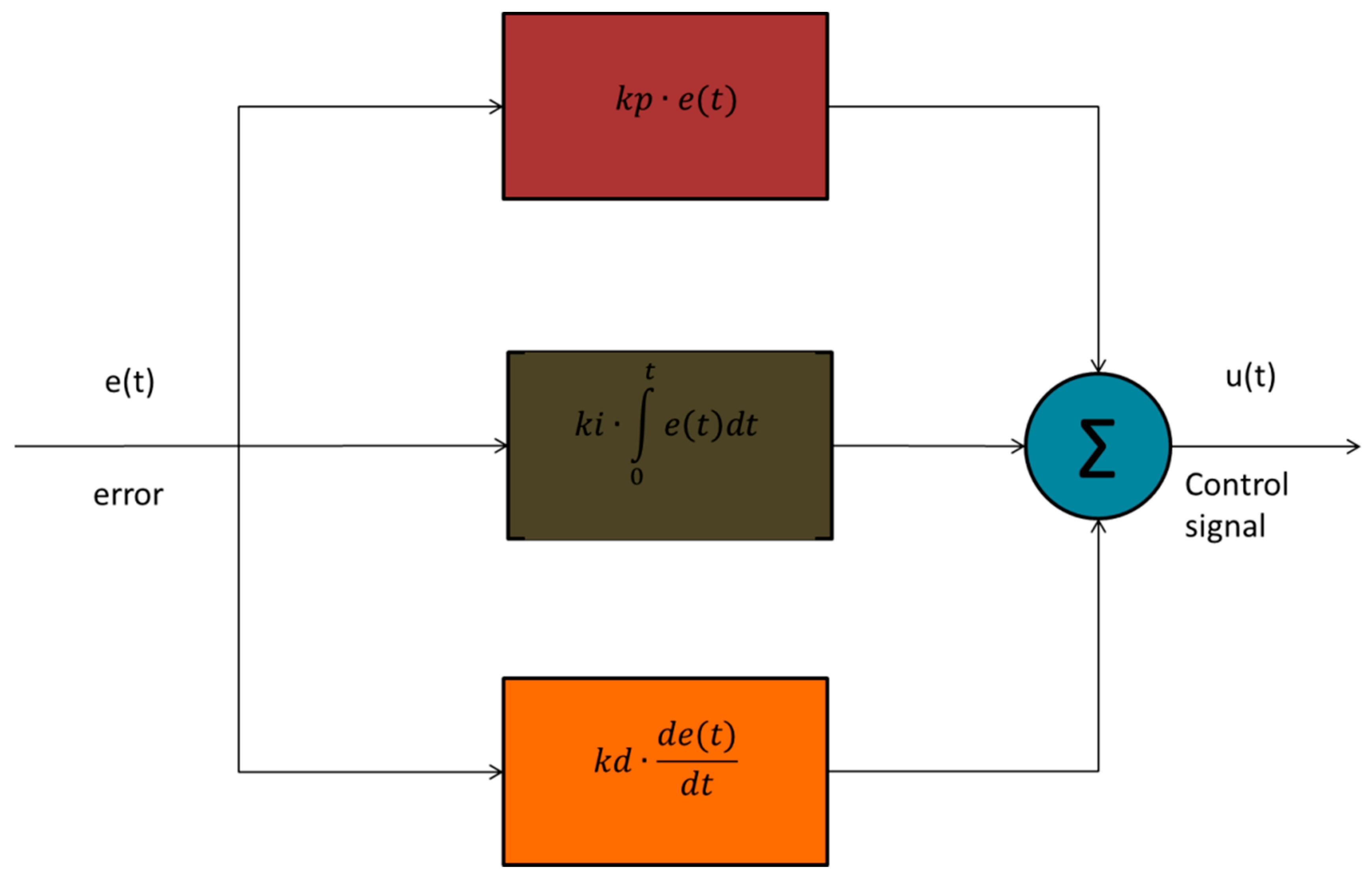
The block diagram of the PID controller is depicted in Figure 1. The input of the PID controller is the error , the error arises by the subtraction of the set point with the true value of . The aim of the PID controller is to produce the appropriate control signal in order to eliminate the error.
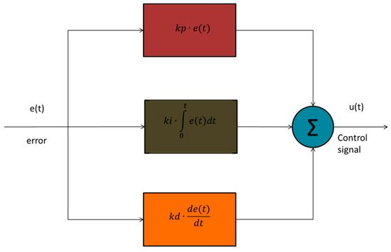
Figure 1.
Block diagram of Proportional Integral Derivative (PID) controller.
In order to increase the system’s response speed and to decrease steady-state error, the proportional gain () was used in order the control signal u(t) to respond to the error immediately. The integral gain () was used for eliminating the offset error but caused overshoot. In order to reduce this overshoot, the derivative gain () was used [27]. The transfer function of the PID controller was:
2.2. FLS
The main advantage of fuzzy logic systems is that they can express complex processes by using fuzzy if/then rules. These rules contain knowledge of the expert and can express relationships among fuzzy variables using linguistic terms [28]. The generic form of a fuzzy rule is:
where is a fuzzy set of th input, is the crisp input vector, c is the output variable, and is a fuzzy set defined by the expert.
The Sugeno [29] type FLS is the most commonly used due to its computational efficiency, as it does not need a defuzzifier. In the simplest case, where a zero-order type Sugeno (the consequents of the rules are constant numbers) is used, the global output of the FLS can be calculated by the Wang-Mendel model [30].
where is the consequent of rule and is the firing strength of the rule .
2.3. Reinforcement Learning
The term reinforcement learning refers to a family of algorithms inspired by human and animal learning. The aim of the reinforcement learning is to find a policy that maximizes the expected discounted reward [31]. The maximization of the expected discounted reward is performed via exploration/exploitation in the space of possible state-action pairs. Actions that give good performance when performed in a given state are rewarded with a positive reinforcement signal (reward), and actions that give poor performance are punished with a negative reinforcement signal (punishment). This signal provides feedback to the system in order to learn the “value” of actions in different states.
2.3.1. Q-Learning
The Q-learning is a reinforcement learning method. In this method the agent calculates the Q-function which evaluates the future discounted rewards of candidate actions performed in states [32]. The Q-function’s output for a given state and an action is denoted as . The Q value of each action when performed in a state is updated as follows:
where is the new value of the state-action combination after the updating from the reward which acquired by performing the action in the state . The algorithm of Q learning assumes that the agent continues from state by performing the optimal policy, thus is the maximum value when the best action is applied in state (the next state which arises after executing the action in state ). The learning rate defines the degree that the new information overrides the old one [33], and the discount factor defines the importance of the future rewards [34]. Generally, the Q-learning agent selects the action to be performed in state and identifies the consequent state . It obtains the reward from the transition , and updates the value for the combination supposing that the optimal policy is applied from state and onwards. A Q-learning agent uses an exploration/exploitation scheme in order to figure a policy that maximizes payoff.
The main characteristic that makes Q-learning suitable to our study is its model-free approach. On the contrary, the main disadvantage of the Q-learning is that it cannot be applied to continuous action-state spaces that our problem involves. In order to confront this problem, fuzzy function approximation can be used.
2.3.2. Fuzzy Q-Learning
One main advantage of FLS is that they can achieve good approximations [35] in the Q-function making possible the usage of the Q-learning in continuous state-space problems (fuzzy Q-learning) [36]. In fuzzy Q-learning, is the crisp set of the inputs that defines the state of the agent. These are converted into fuzzy values and each fuzzy rule corresponds to a state. Thus, the firing strength of each rule determines the degree to which the agent is in a state. Additionally, the rules do not have standard consequents; meaning there are no predefined state-action pairs, and the consequents of each rule arises via the exploration/exploitation algorithm. So, the FLS has competing actions for each rule and the rules have the form:
where is the potential action in fuzzy rule . For each candidate action in rule there is a corresponding value . This value defines how “good” the action is performed, when the rule is fired. The state is defined by , where , are fuzzy sets.
The fuzzy Q-learning algorithm has to follow:
- Observe state
- Select an action for each fired rule according to the exploration/exploitation algorithm.
- Calculate the global output from the following equation:where corresponds to the chosen action of rule .
- Calculate the corresponding value as follows:where is the corresponding q-value of the fired rule for the choice of the action by the exploration/exploitation strategy.
- Apply the action and observe the new state .
- Calculate the reward
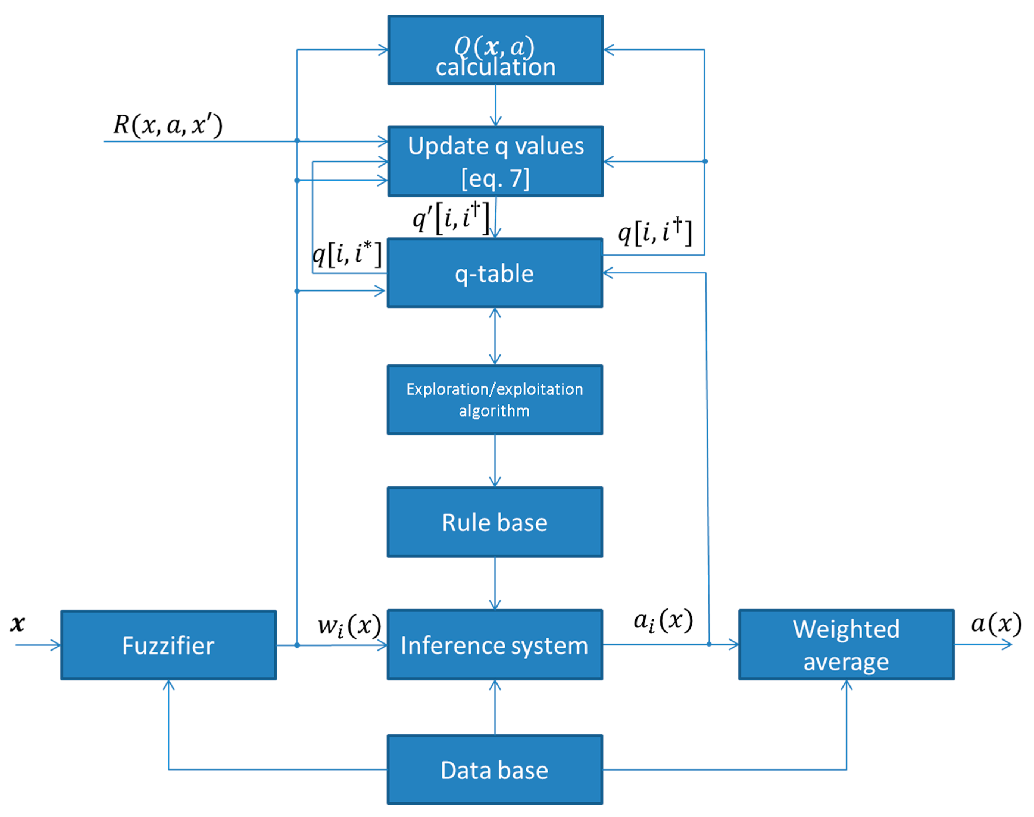
- Update the q values as follows:where and is the choice of the action that has the maximum Q value for the fired rule . The block diagram of a fuzzy Q-learning agent is depicted in Figure 2. Thus, the q values are updated as:
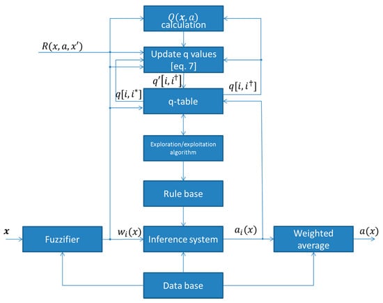 Figure 2. General block diagram of fuzzy Q-learning agent.
2.4. MAS and Q-Learning
A system that consists of a set of agents that are able to each interact with the environment and with the other agents is called MAS [37]. The MAS are considered to be the basic field of the distributed artificial intelligence. A MAS is developed in order to solve a complex problem that a single agent cannot solve (or it is very difficult to solve), or to solve a problem which is distributed by its nature.
A MAS consists of a set of agents that act together in order to solve a problem. In problems which are distributed, the agents must cooperate together so as to maximize the total discounted reward [38]. This type of problem can be expressed as an extension of a Markov Decision Process (MDP) for a single agent [39]. Solving this MDP results in the extraction of the policy. According to Q-learning, a MAS can be expressed as a single agent with multiple states and an action vector, which can apply the conventional Q-learning algorithm [40]. Following this algorithm has the disadvantage that the state-action space of the agent grows exponentially according the number of the state variables and the action vector. In order to overcome this disadvantage, a variety of approaches have been developed, with the most well-known being coordinated reinforcement learning, distributed value function, and independent learners. The simplest approach of these three approaches is the independent learners because, according to this method, each agent acts in an individual manner. The agents act independently and each agent learns its own policy. By this way, an agent does not know either the Q-values or the policies of the other agents. Each agent stores and updates its own Q-table (Equation (8)) noting that each is based on the global state [41].
The main disadvantage of this method is that the environment is no longer stationary [42] and the convergence cannot be guaranteed. This happens because an agent ignores the presence of other agents. An agent can sense possible actions of other agents indirectly as changes of the environment occur. Despite this disadvantage, this method has been previously successfully applied in many control problems [40].
3. Desalination Model, Control Strategy and Implementation
3.1. Desalination Model
In this work an adaptive neuro fuzzy inference system (ANFIS) model of a reverse osmosis desalination plant was used. The model was data-driven and had one input and one output. The input was the DC voltage, from 0 to 32 V, and the output was the flow rate of the produced water, from 0 to 105 L/h. The data came from a pilot desalination unit installed in the Agricultural University of Athens. The desalination unit consisted of two 25- to 40-inch spiral-wound seawater Filmtec membrane modules. A rotary vane pump, of positive displacement, pressurized the water to one of the two cylinders of the Clark pump. The Clark pump was used as an energy recovery unit, instead of the high-pressure pumps that can be found in the conventional desalination units. The high-pressure brine was introduced into the second cylinder and exchanged the hydraulic energy with the feed water pressure of 13 bar. By this exchange, the pressure of the feed water was risen to 50 bar, which is the appropriate pressure of the membrane. More information about the desalination unit can be found on [43,44,45] and more information about the development of the ANFIS model can be found on [46].
3.2. Control Strategy
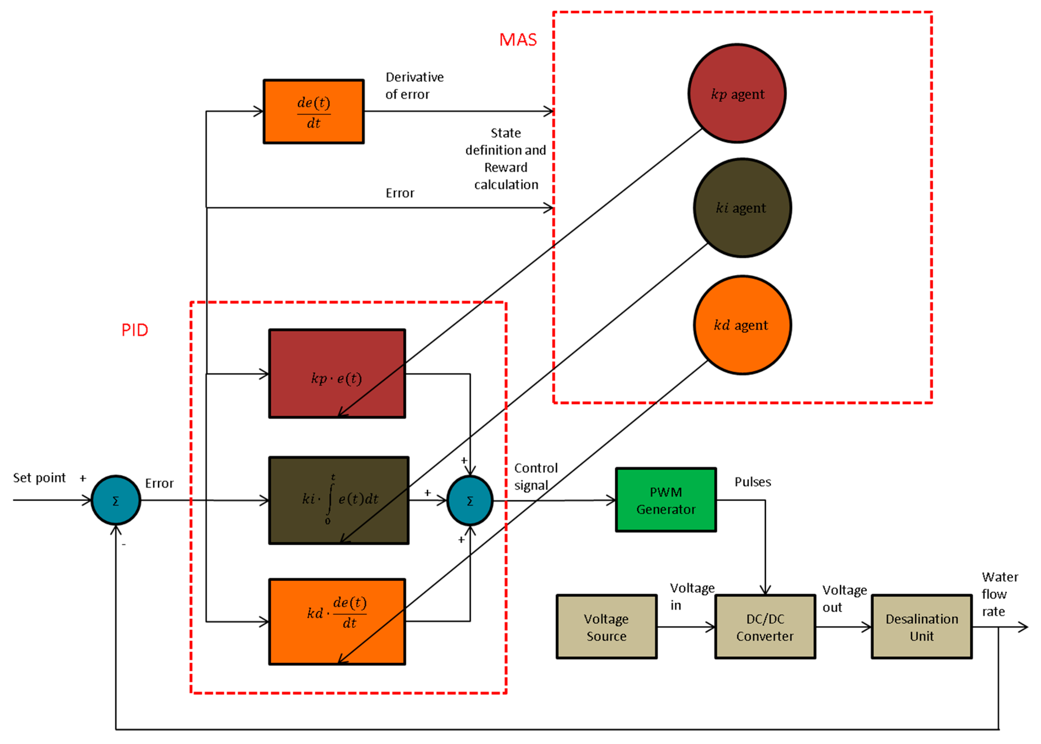
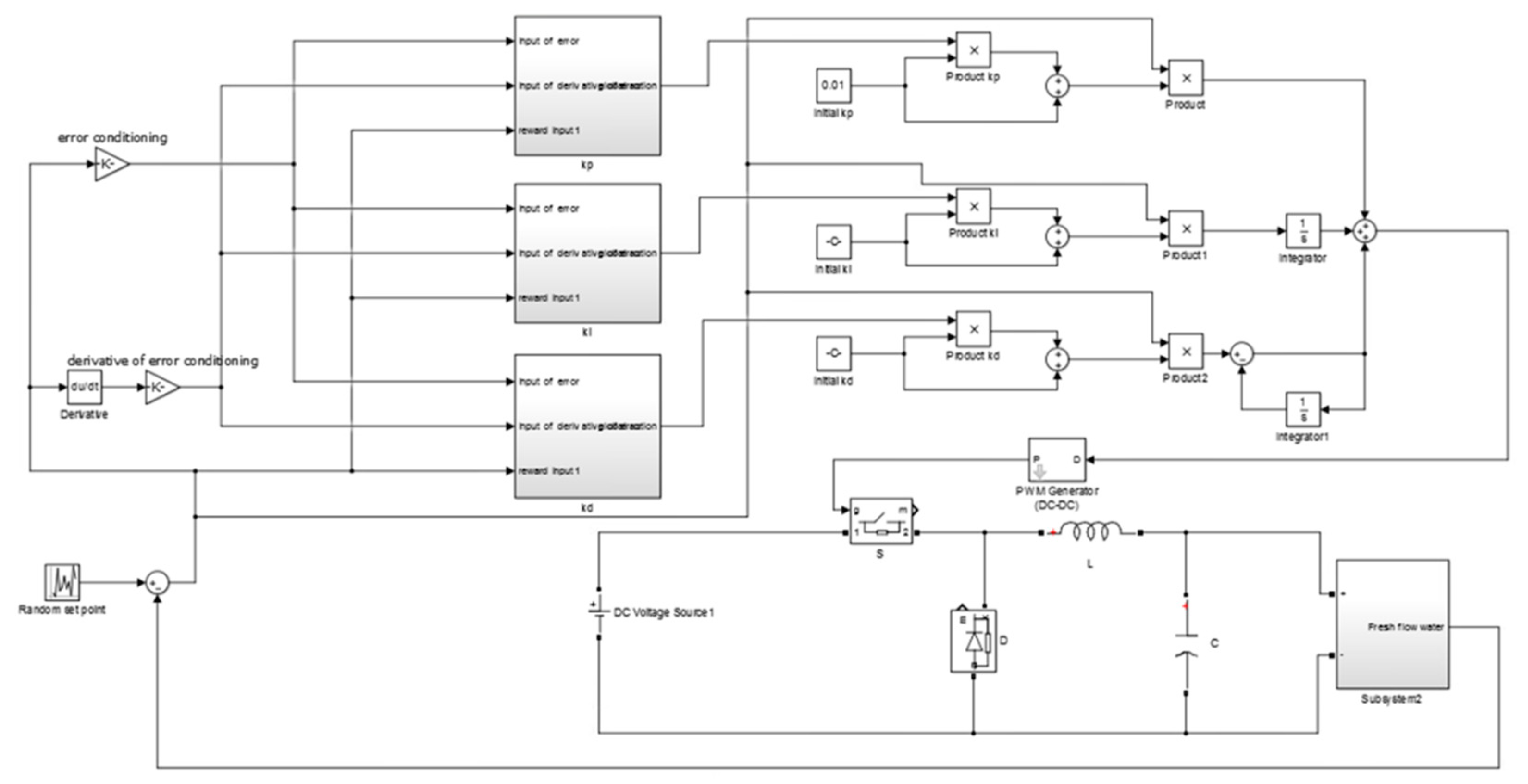
The control strategy of the desalination plant is depicted in Figure 3. The error arose from the subtraction of the set point (desire water flow rate) and the true value of the flow rate. The error signal was the input of the PID controller. The output of the PID controller was the reference voltage of the Pulse Width Modulation (PWM) generator. The PWM generator [47] produced pulses, which drove the switch of the converter. The converter received voltage in the input and, accordingly, the duty cycle of the pulses changed its output voltage. The output voltage of the converter was the input voltage of the desalination plant. The signal error and the derivative of error were the inputs of the MAS. The action of each agent adjusted each gain of the PID controller.

Figure 3.
Block diagram of proposed control strategy.
The converter of the system was a buck converter [48]. The converter changed the output voltage according the duty cycle of the pulses:
where is the output voltage of the converter, is the duty cycle of the pulses, and is the input voltage of the converter.
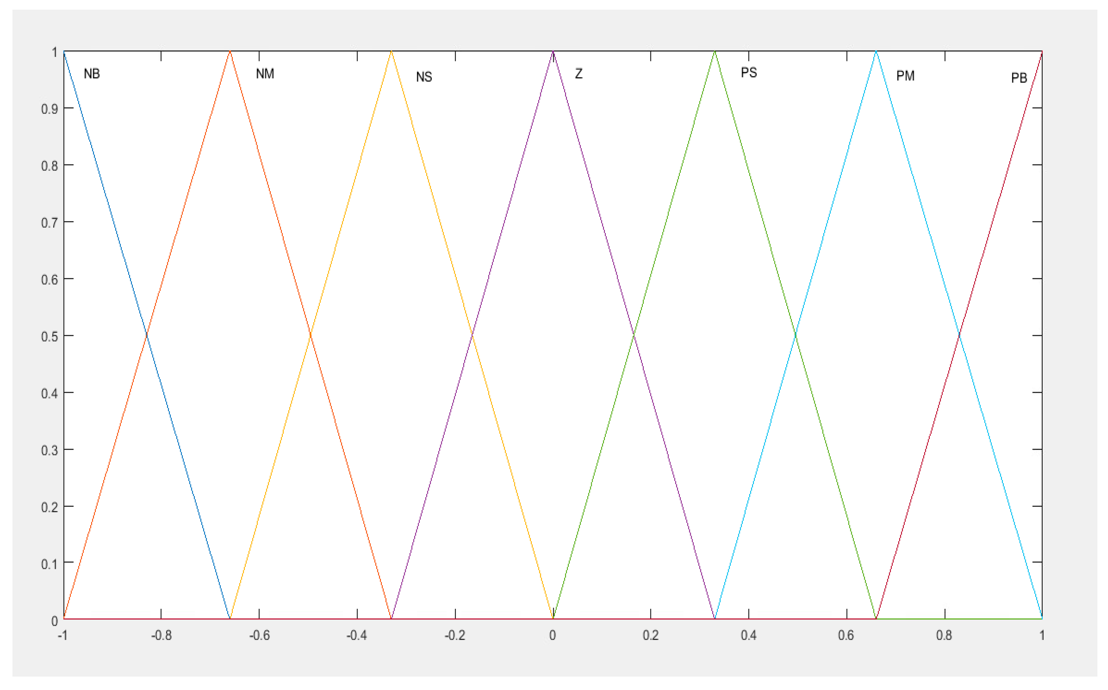
The MAS had two input signals, which were the error and the derivative of error. These signals defined the global state of the MAS. The MAS consisted of three agents, each one for one gain of the PID controller. There were the agent, the agent, and the which were dedicated to adjust the gains , and respectively. The input signals were conditioning in the range of {−1, 1} and, through the fuzzy approximator, defined the current states of the MAS. The membership functions for each state variable (for both inputs) were seven (Figure 4). The quantization of the inputs in the seven areas, with 50% overlapping, provided enough details in order to cover the range of each input. In addition to that, the state space remained small (two inputs with seven MFs each results in a total of 49 states) and was easy to explore. These states were represented by an equal number of fuzzy rules and, consequently, the MAS could simultaneously be from one state to four (each state had each firing strength). The NB, NM, NS, Z, PS, PM, and PB denote Negative Big, Negative Medium, Negative Small, Zero, Positive Small, Positive Medium, and Positive Big, respectively.
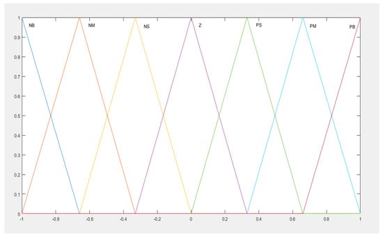
Figure 4.
Input membership functions, Negative Big (NB), Negative Medium (NM), Negative Small (NS), Zero (Z), Positive Small (PS), Positive Medium (PM) and Positive Big (PB).
The output of each agent defined the percentage change of each gain according to the initial values of the gains tuned by the Z-N method. Each agent’s output had a group of five fuzzy actions (fuzzy singletons). The set of the actions for all the agents was the same: . where “+” is the operator of union and “–” represents a membership degree to a value of the membership function domain. The state-action space of each agent contained 245 combinations.
According to Q-learning, in order for each agent to acquire knowledge it interacts with the environment through an exploration/exploitation algorithm. This algorithm defines whether the agent performs exploration or exploitation. When the MAS becomes a new state, the agent explores for a certain number of rounds per state (500 rounds/state), and then checks and applies the action that has not been applied at all (if there are any), while the other two agents are keeping each value constant (zero). After the MAS performs the first 500 rounds, the second agent explores for 500 rounds/state, and then after 1000 rounds, the third agent performs exploration for another 500 rounds/state. By this way the extensive exploration phase for each agent has little overlapping with the other two, and allows the algorithm to converge (the performing of all the agent’s extensive exploration simultaneously may lead to oscillations). After the extensive exploration phase, each agent performs exploitation for 99% and exploration for 1% for a given state [26].
The reward () is defined as follows:
where is the value of the error in the resulting state. The fraction takes values in the range {0, 1}. If the value of error is zero, the value of this quantity becomes “1”, otherwise, high positive or negative values of error reduce this quantity. The outcome of subtracting this quantity with the quantity that has the error in the succeeding state, gives a reward which can take positives and negative values. Positive values show that the error in the succeeding state is reduced while negative values show that the error in the succeeding state is raised. Greater values of reward indicate greater reduction of the error and vice versa [25].
3.3. Implementation
The whole system implemented in Matlab/Simulink (Mathworks, R2015a, Massachusetts, U.S.A) can be seen in Figure 5. There were three agents; each one had two inputs (error and derivative of error). The output of each agent adapted each gain of the PID controller. The output of the PID controller was the input of the PWM generator. The PWM generator had a frequency of . The pulses produced by the PWM generator drove the switch of the buck converter. The converter had a capacitor of and an inductor of . The input voltage of the converter was a direct current voltage source. The output of the converter was the voltage fed into the desalination plant. The simulation time was set to with a simulation time step of . During the simulation, different values of the set point (flow rate of the produced water) were set. The set point was changing every 1 s. The range of the set point was from 0 to . The aim of the simulation was to compare a conventional PID controller tuned by Z-N with the proposed control strategy. The values of the gains of the PID controller which arose from the Z-N method were , and . The learning rate was set to and the discount factor set to . The time round for the MAS was set to 0.01 s.

Figure 5.
System implementation in Matlab/Simulink.
4. Simulation Results
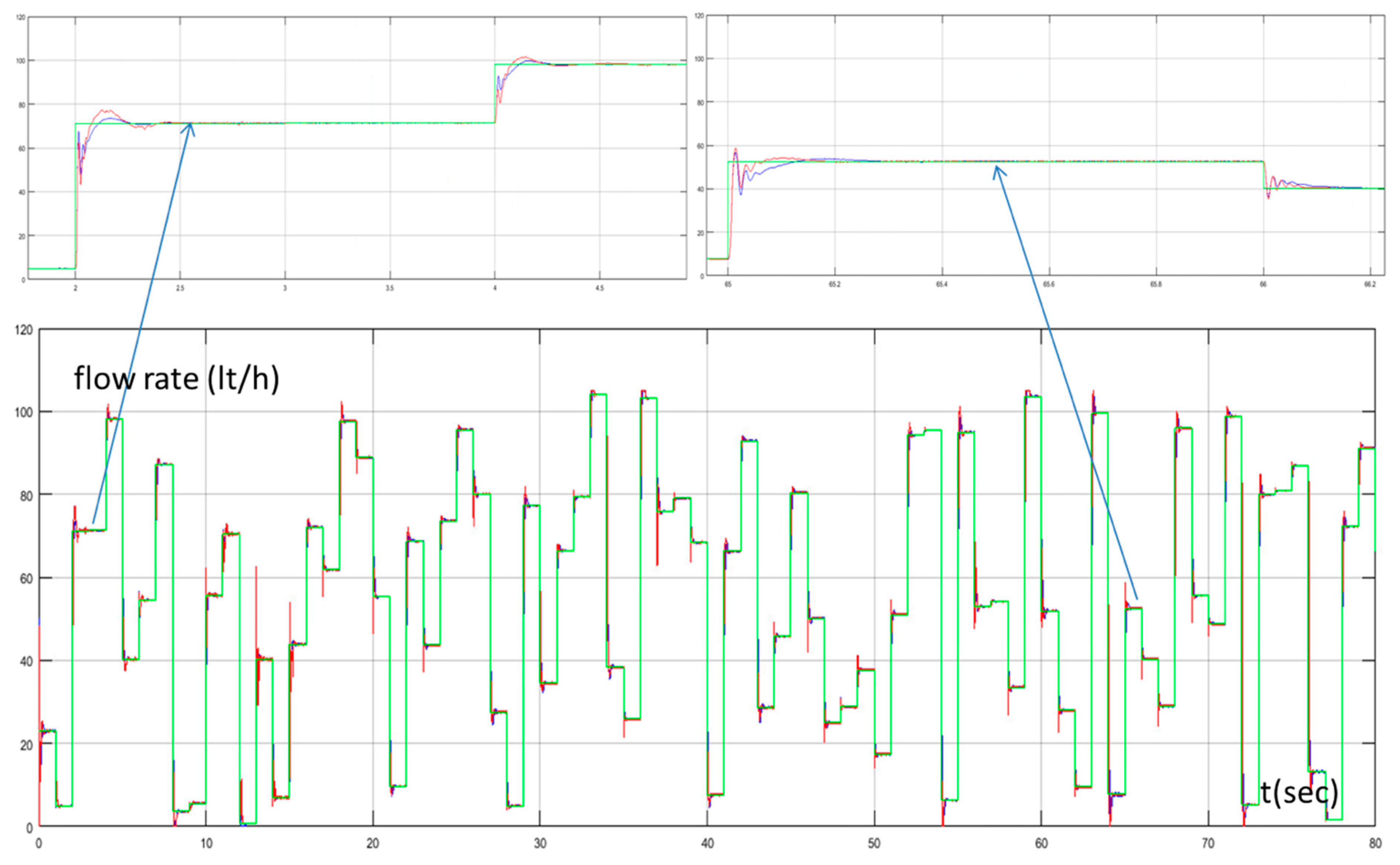
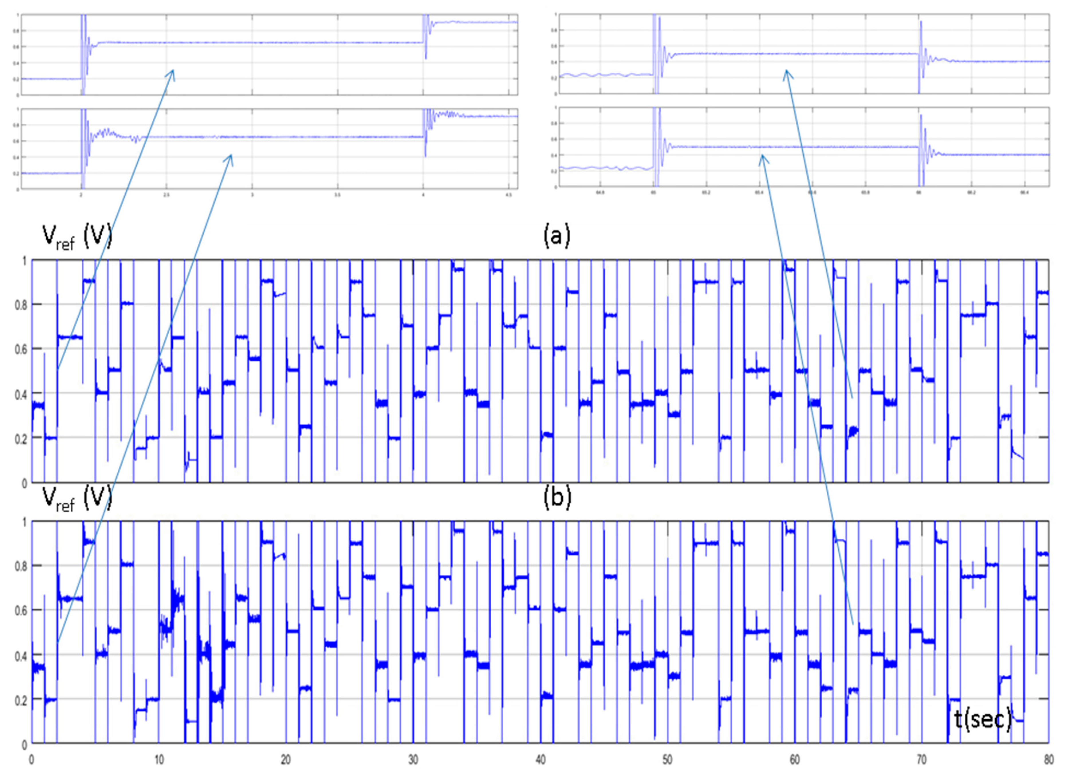
In Figure 6, the set point of the water flow rate, the water flow rate of the desalination unit controlled by the PID controller tuned by the Z-N, and the water flow rate of the proposed method are presented. Figure 7 presents the control signals (reference voltage of the PWM generator) of both methods. In the beginning of the simulation, where the MAS performed extensive exploration, we could see that the output of the system of the proposed method had a higher overshoot and a higher settling time compared with the conventional PID controller. On the contrary, during the exploitation phase, we could see that the proposed method performed better. The settling time was much less compared to the PID controller tuned by Z-N and with a small overshoot. These two points (Figure 6 and Figure 7) were at 2 s (exploration phase) and at 65 s (exploitation phase).
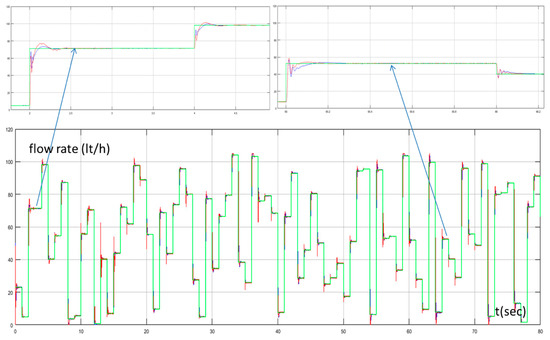
Figure 6.
Water flow rate with Proportional Integral Derivative (PID) controller tuned by Z–N (blue line), water flow rate with fuzzy Q-learning Multi-Agent System (MAS) PID controller (red line), and set point of water flow rate (green line).
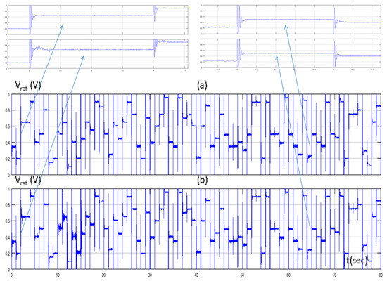
Figure 7.
(a) Reference voltage of PID controller tuned by Z–N; and (b) reference voltage of fuzzy Q-learning MAS PID controller.
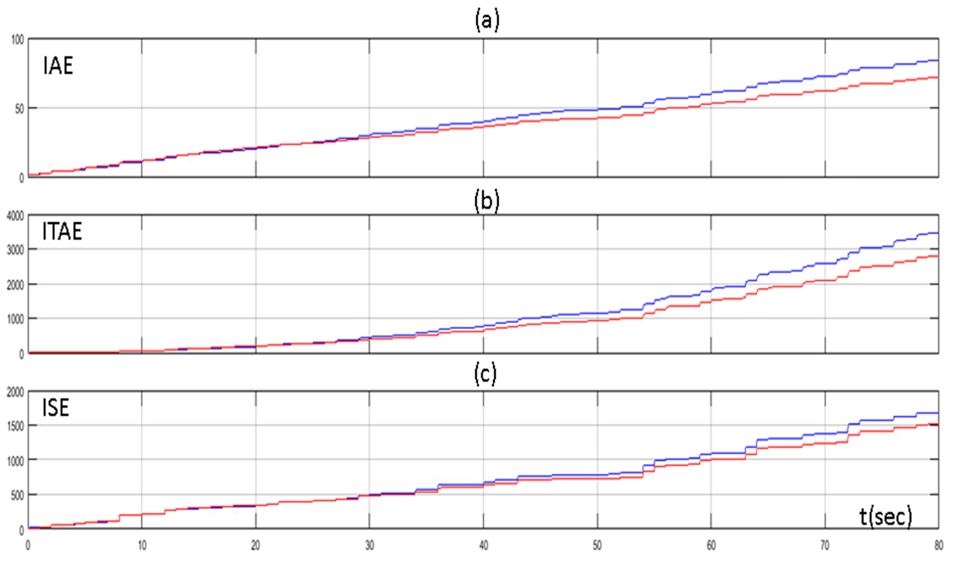
The improvement of the performance of the proposed method was highlighted in Figure 8, where the values of the Integral Absolute Error (IAE), the Integral Time Absolute Error (ITAE), and the Integral Square Error (ISE) through time are presented. The IAE, the ITAE, and the ISE are defined as below:
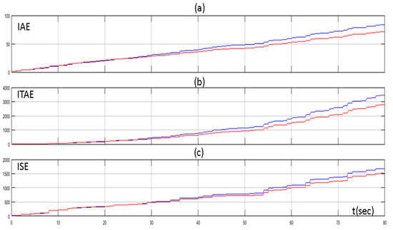
Figure 8.
(a) Integral Absolute Error (IAE) of PID controller tuned by Z–N (blue line) and fuzzy Q-learning MAS PID controller (red line); (b) Integral Time Absolute Error (ITAE) of PID controller tuned by Z–N (blue line) and fuzzy Q-learning MAS PID controller (red line); and (c) Integral Square Error (ISE) of PID controller tuned by Z–N (blue line) and fuzzy Q-learning MAS PID controller (red line).
We can see that the values of the IAE, ITAE, and ISE were the same for both methods in the beginning (exploration phase). As the MAS turned from the exploration phase to exploitation phase, the values of the IAE, ITAE, and ISE turned so that they were lower for the proposed method than the conventional PID controller.
Figure 9 presents the percentage change of the three gains of the controller (actions of the three agents) of the proposed control method through time, in respect to the various changes of the set point.
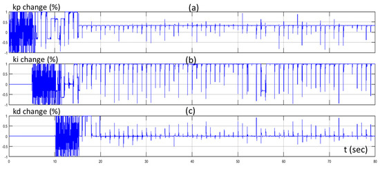
Figure 9.
Percentage change of (a) proportional gain (kp); (b) integral gain (ki); and (c) derivative gain (kd) through time.
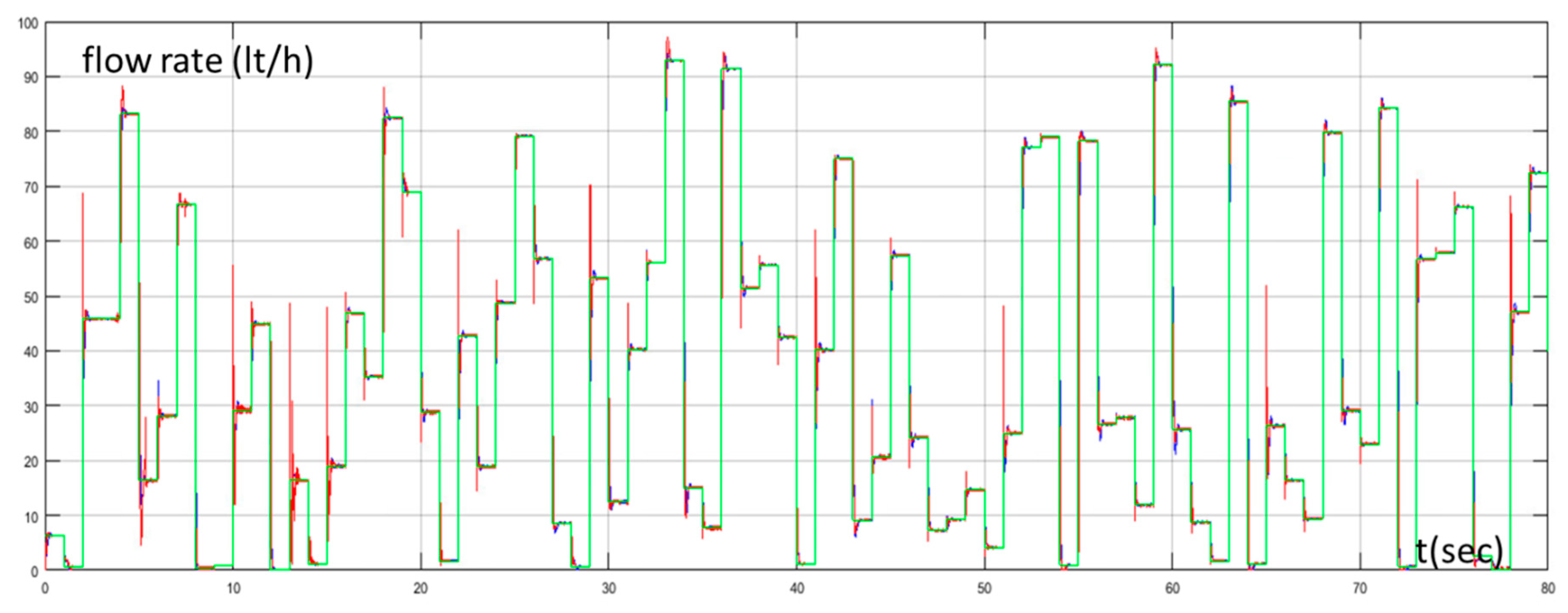
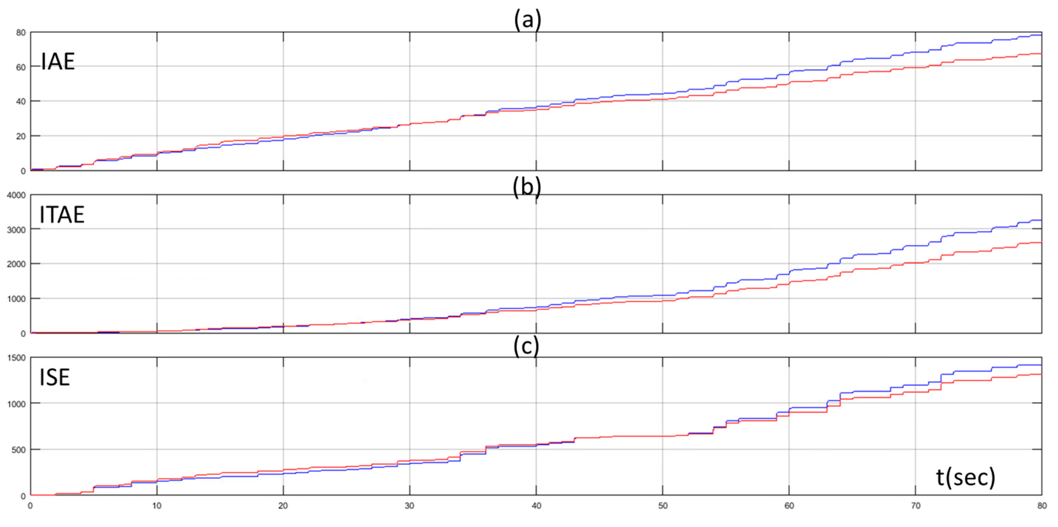
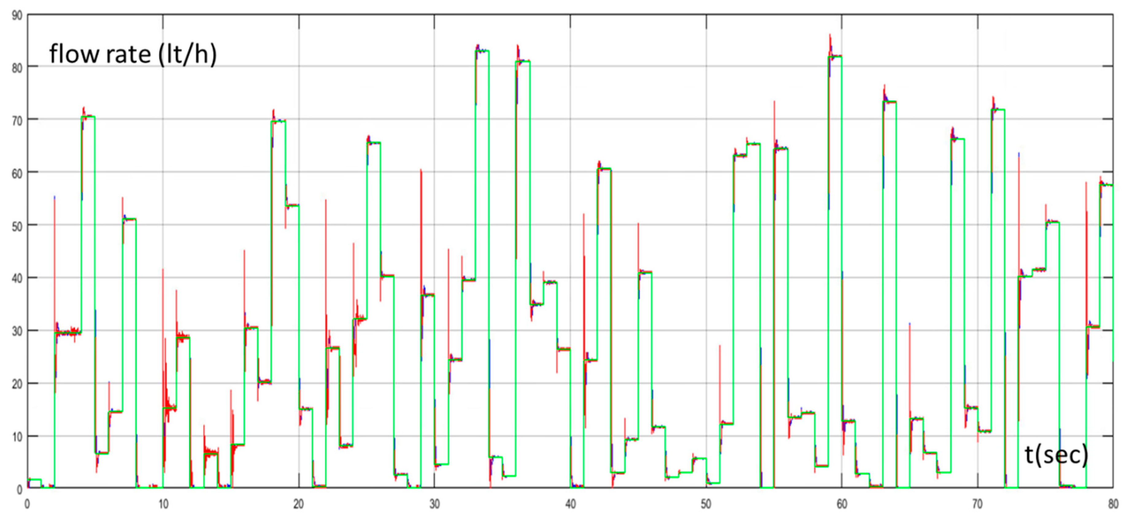
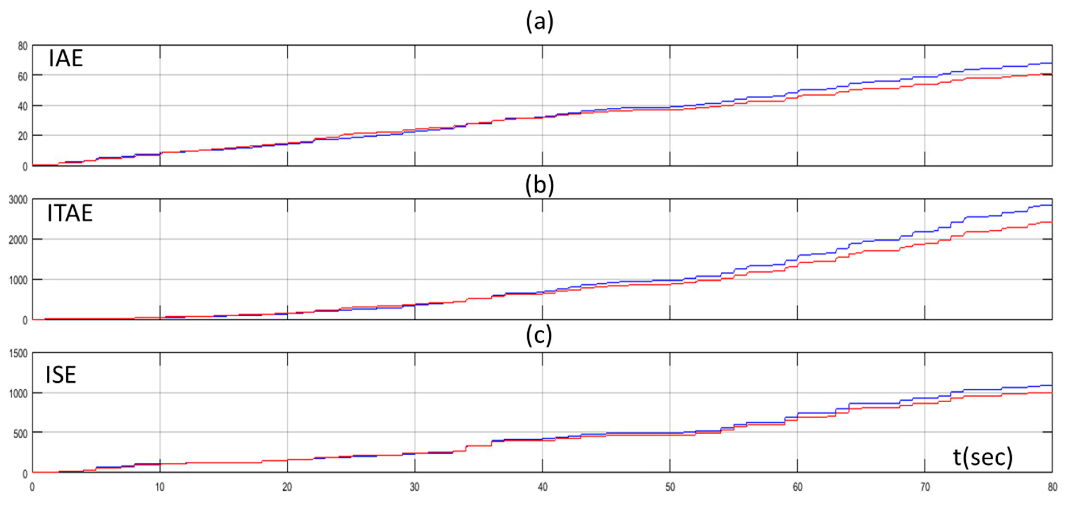
The proposed approach was tested under another two different scenarios with different random set points. In Figure 10 the set point of the water flow rate, the water flow rate of the desalination unit controlled by the PID controller tuned by the Z-N, and the water flow rate of the proposed method for the first scenario are presented while Figure 11 presents the values of the IAE, ITAE, and ISE through time for the same scenario. Figure 12 and Figure 13 present the same quantities with Figure 10 and Figure 11 respectively for the second scenario. We can see that the values of the IAE, ITAE, and ISE were the same for both methods in the beginning (exploration phase) for both scenarios. As the MAS turned from the exploration phase to the exploitation phase, the values of the IAE, ITAE, and ISE turned so that they were lower for the proposed method, than the conventional PID controller, for both scenarios. The performance of the proposed method for these scenarios highlights its superiority compared to the Z-N method and confirms its effectiveness and robustness.
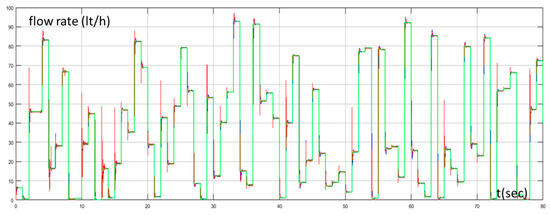
Figure 10.
Water flow rate with PID controller tuned by Z–N (blue line), water flow rate with fuzzy Q-learning MAS PID controller (red line), and set point of water flow rate (green line) for scenario 1.
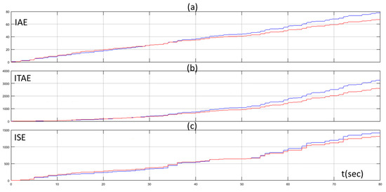
Figure 11.
(a) IAE of PID controller tuned by Z-N (blue line) and fuzzy Q-learning MAS PID controller (red line); (b) ITAE of PID controller tuned by Z-N (blue line) and fuzzy Q-learning MAS PID controller (red line); and (c) ISE of PID controller tuned by Z-N (blue line) and fuzzy Q-learning MAS PID controller (red line) for scenario 1.
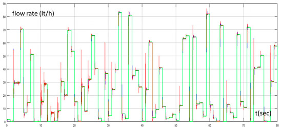
Figure 12.
Water flow rate with PID controller tuned by Z–N (blue line), water flow rate with fuzzy Q-learning MAS PID controller (red line), and set point of water flow rate (green line) for scenario 2.
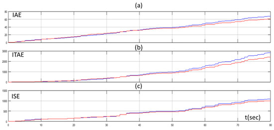
Figure 13.
(a) IAE of PID controller tuned by Z-N (blue line) and fuzzy Q-learning MAS PID controller (red line); (b) ITAE of PID controller tuned by Z-N (blue line) and fuzzy Q-learning MAS PID controller (red line); and (c) ISE of PID controller tuned by Z-N (blue line) and fuzzy Q-learning MAS PID controller (red line) for scenario 2.
5. Discussion
This paper presents a fuzzy Q-learning MAS for adjusting online the three gains of a PID controller. The controller was used to control the flow rate of a desalination unit. The gains of the controller were initialized by the Z-N method. The input variables of the MAS were the error and the derivative of error. The output of each agent was the percentage change of the gain that each agent was dedicated to adapt. Fuzzy logic was used in combination with Q-learning in each agent in order to confront the continuous state-action space. The simulation results indicated the better performance of the proposed method and especially the lower values of the IAE, ITAE, and ISE. Using a single agent with multiple input variables and an action vector resulted in the exponential growth of the state-action space. By decomposing the problem in many simple problems using the independent learners’ approach, the state-action space was reduced. On the other hand, the drawback of this approach was that it could not guarantee convergence. The agents were acting and updating their tables without taking into account the actions of the other agents, In future, our aim is to focus on the implementation of other reinforcement learning approaches for MAS in order to overcome this limitation. Additionally, the combination between online learning algorithms and offline optimization methods for tuning the membership function of both the inputs and the outputs of the agents can be tested in order to improve the overall performance of the system.
Author Contributions
Methodology, P.K.; software, P.K.; supervision, A.I.D.; visualization, A.I.D.; writing—original draft, P.K.; writing—review and editing, A.I.D.
Funding
This research received no external funding.
Conflicts of Interest
The authors declare no conflicts of interest.
References
- Libotean, D.; Giralt, J.; Giralt, F.; Rallo, R.; Wolfe, T.; Cohen, Y. Neural network approach for modeling the performance of reverse osmosis membrane desalting. J. Membr. Sci. 2009, 326, 408–419. [Google Scholar] [CrossRef]
- Meshram, P.M.; Kanojiya, R.G. Tuning of PID Controller using Ziegler-Nichols Method for Speed Control of DC Motor. In Proceedings of the IEEE International Conference on Advances in Engineering, Science and Management (ICAESM-2012), Nagapattinam, Tamil Nadu, India, 30–31 March 2012. [Google Scholar]
- Amaral, J.F.M.; Tanscheit, R.; Pacheco, M.A.C. Tuning PID Controllers through Genetic Algorithms. In Proceedings of the 2001 WSES International Conference on Evolutionary Computation, Puerto De La Cruz, Spain, 11–15 February 2001. [Google Scholar]
- Jayachitra, A.; Vinodha, R. Genetic Algorithm Based PID Controller Tuning Approach for Continuous Stirred Tank Reactor. Adv. Artif. Intell. 2014, 2014, 9. [Google Scholar] [CrossRef]
- Sheng, L.; Li, W. Optimization Design by Genetic Algorithm Controller for Trajectory Control of a 3-RRR Parallel Robot. Algorithms 2018, 11, 7. [Google Scholar] [CrossRef]
- Ibrahim, H.E.-S.A.; Ahmed, M.S.S.; Awad, K.M. Speed control of switched reluctance motor using genetic algorithm and ant colony based on optimizing PID controller. ITM Web Conf. 2018, 16, 01001. [Google Scholar] [CrossRef]
- Aouf, A.; Boussaid, L.; Sakly, A. A PSO algorithm applied to a PID controller for motion mobile robot in a complex dynamic environment. In Proceedings of the International Conference on Engineering & MIS (ICEMIS), Monastir, Tunisia, 8–10 May 2017. [Google Scholar]
- Ansu, E.K.; Koshy, T. Comparison of Adaptive PID controller and PSO tuned PID controller for PMSM Drives. Int. J. Adv. Eng. Res. Dev. 2018, 5, 812–820. [Google Scholar]
- Zeng, G.-Q.; Chen, J.; Dai, Y.-X.; Li, L.-M.; Zheng, C.-W.; Chen, M.-R. Design of fractional order PID controller for automatic regulator voltage system based on multi-objective extremal optimization. Neurocomputing 2015, 160, 173–184. [Google Scholar] [CrossRef]
- Abbasi, E.; Naghavi, N. Offline Auto-Tuning of a PID Controller Using Extended Classifier System (XCS) Algorithm. J. Adv. Comput. Eng. Technol. 2017, 3, 41–44. [Google Scholar]
- Muhammad, Z.; Yusoff, Z.M.; Kasuan, N.; Nordin, M.N.N.; Rahiman, M.H.F.; Taib, M.N. Online Tuning PID using Fuzzy Logic Controller with Self-Tuning Method. In Proceedings of the IEEE 3rd International Conference on System Engineering and Technology, Shah Alam, Malaysia, 19–20 August 2013. [Google Scholar]
- Dounis, A.I.; Kofinas, P.; Alafodimos, C.; Tseles, D. Adaptive fuzzy gain scheduling PID controller for maximum power point tracking of photovoltaic system. Renew. Energy 2013, 60, 202–214. [Google Scholar] [CrossRef]
- Qin, Y.; Sun, L.; Hua, Q.; Liu, P. A Fuzzy Adaptive PID Controller Design for Fuel Cell Power Plant. Sustainability 2018, 10, 2438. [Google Scholar] [CrossRef]
- Luoren, L.; Jinling, L. Research of PID Control Algorithm Based on Neural Network. Energy Procedia 2011, 13, 6988–6993. [Google Scholar]
- Badr, A.Z. Neural Network Based Adaptive PID Controller. IFAC Proc. Vol. 1997, 30, 251–257. [Google Scholar] [CrossRef]
- Rad, A.B.; Bui, T.W.; Li, Y.; Wong, Y.K. A new on-line PID tuning method using neural networks. In Proceedings of the IFAC Digital Control: Past, Present and Future of PID Control, Terrassa, Spain, 5–7 April 2000. [Google Scholar]
- Du, X.; Wang, J.; Jegatheesan, V.; Shi, G. Dissolved Oxygen Control in Activated Sludge Process Using a Neural Network-Based Adaptive PID Algorithm. Appl. Sci. 2018, 8, 261. [Google Scholar] [CrossRef]
- Agrawal, A.; Goyal, V.; Mishra, P. Adaptive Control of a Nonlinear Surge Tank-Level System Using Neural Network-Based PID Controller. In Applications of Artificial Intelligence Techniques in Engineering; Springer: Singapore, 2018; pp. 491–500. [Google Scholar]
- Hernandez-Alvarado, R.; Garcia-Valdovinos, L.G.; Salgado-Jimenez, T.; Gómez-Espinosa, A.; Navarro, F.F. Self-tuned PID Control based on Backpropagation Neural Networks for Underwater Vehicles. In Proceedings of the OCEANS 2016 MTS/IEEE, Monterey, CA, USA, 19–23 September 2016. [Google Scholar]
- Merayo, N.; Juárez, D.; Aguado, J.C.; de Miguel, I.; Durán, R.J.; Fernández, P.; Lorenzo, R.M.; Abril, E.J. PID Controller Based on a Self-Adaptive Neural Network to Ensure QoS Bandwidth Requirements in Passive Optical Networks. IEEE/OSA J. Opt. Commun. Netw. 2017, 9, 433–445. [Google Scholar] [CrossRef]
- Kim, J.-S.; Kim, J.-H.; Park, J.-M.; Park, S.-M.; Choe, W.-Y.; Heo, H. Auto Tuning PID Controller based on Improved Genetic Algorithm for Reverse Osmosis Plant. Int. J. Electron. Inf. Eng. 2008, 2, 11. [Google Scholar]
- Rathore, N.S.; Kundariya, N.; Narain, A. PID Controller Tuning in Reverse Osmosis System based on Particle Swarm Optimization. Int. J. Sci. Res. Publ. 2013, 3, 1–5. [Google Scholar]
- Jana, I.; Asuntha, A.; Brindha, A.; Selvam, K.; Srinivasan, A. Tuning of PID Controller for Reverse Osmosis (RO) Desalination System Using Particle Swarm Optimization (PSO) Technique. Int. J. Control Theory Appl. 2017, 10, 83–92. [Google Scholar]
- Glorennec, P.Y.; Jouffe, L. Fuzzy Q-learning. In Proceedings of the 6th International Fuzzy Systems Conference, Barcelona, Spain, 5 July 1997; pp. 659–662. [Google Scholar]
- Kofinas, P.; Dounis, A. Fuzzy Q-learning Agent for Online Tuning of PID Controller for DC Motor Speed Control. Algorithms 2018, 11, 148. [Google Scholar] [CrossRef]
- Kofinas, P.; Dounis, A.I.; Vouros, G.A. Fuzzy Q-learning for multi-agent decentralized energy management in microgrids. Appl. Energy 2018, 219, 53–67. [Google Scholar] [CrossRef]
- Abdulameer, A.; Sulaiman, M.; Aras, M.S.M.; Saleem, D. Tuning Methods of PID Controller for DC Motor Speed Control. Indones. J. Electr. Eng. Comput. Sci. 2016, 3, 343–349. [Google Scholar] [CrossRef]
- Tsoukalas, L.; Uhring, R. Fuzzy and Neural Approaches in Engineering; MATLAB Supplement; John Wiley & Sons: Hoboken, NJ, USA, 1997. [Google Scholar]
- Takagi, T.; Sugeno, M. Fuzzy identification of systems and its applications to modeling and control. IEEE Trans. Syst. Man Cybern. 1985, 15, 116–132. [Google Scholar] [CrossRef]
- Wang, L.-X. A Course in Fuzzy Systems and Control; Prentice Hall PTR: Upper Saddle River, NJ, USA, 1997. [Google Scholar]
- Russel, S.; Norving, P. Artificial Intelligence: A Modern Approach; Prentice Hall: Upper Saddle River, NJ, USA, 1995. [Google Scholar]
- Watkins, C.J.C.H. Learning from Delayed Reinforcement Signals. Ph.D. Thesis, University of Cambridge, Cambridge, UK, 1989. [Google Scholar]
- Sutton, R.; Barto, A. Reinforcement Learning: An Introduction; MIT Press: Cambridge, MA, USA, 1998. [Google Scholar]
- Vincent, F.S.-L.; Fonteneau, R.; Ernst, D. How to Discount Deep Reinforcement Learning: Towards New Dynamic Strategies. arXiv, 2015; arXiv:1512.02011. [Google Scholar]
- Van Hasselt, H. Reinforcement Learning in Continuous State and Action Spaces. In Reinforcement Learning: State of the Art; Springer: Berlin/Heidelberg, Germany, 2012; pp. 207–251. [Google Scholar]
- Castro, J.L. Fuzzy logic controllers are universal approximators. IEEE Trans. SMC 1995, 25, 629–635. [Google Scholar] [CrossRef]
- Sycara, K. Multiagent systems. AI Mag. 1998, 19, 79–92. [Google Scholar]
- Shi, B.; Liu, J. Decentralized control and fair load-shedding compensations to prevent cascading failures in a smart grid. Int. J. Electr. Power Energy Syst. 2015, 67, 582–590. [Google Scholar] [CrossRef]
- Puterman, M.L. Markov Decision Processes: Discrete Stochastic Dynamic Programming; Wiley: New York, NY, USA, 1994. [Google Scholar]
- Kok, J.R.; Vlassis, N. Collaborative Multiagent Reinforcement Learning by Payoff Propagation. J. Mach. Learn. Res. 2006, 7, 1789–1828. [Google Scholar]
- Claus, C.; Boutilier, C. The dynamics of reinforcement learning in cooperative multiagent systems. In Proceedings of the National Conference on Artificial Intelligence (AAAI), Madison, WI, USA, 26–30 July 1998. [Google Scholar]
- Laurent, G.J.; Matignon, L.; Fort-Piat, N.L. The world of independent learners is not markovian. KES J. 2011, 15, 55–64. [Google Scholar] [CrossRef]
- Mohamed, E.S.; Papadakis, G.; Mathioulakis, E.; Belessiotis, V. A direct-coupled photovoltaic seawater reverse osmosis desalination system toward battery-based systems—A technical and economical experimental comparative study. Desalination 2008, 221, 17–22. [Google Scholar] [CrossRef]
- Mohamed, E.S.; Papadakis, G.; Mathioulakis, E.; Belessiotis, V. An experimental comparative study of the technical and economic performance of a small reverse osmosis desalination system equipped with hydraulic energy recovery unit. Desalination 2006, 194, 239–250. [Google Scholar] [CrossRef]
- Mohamed, E.S.; Papadakis, G.; Mathioulakis, E.; Belessiotis, V. The effect of hydraulic energy recovery in a small sea water reverse osmosis desalination system; experimental and economical evaluation. Desalination 2005, 184, 241–246. [Google Scholar] [CrossRef]
- Kofinas, P.; Dounis, A.I.; Mohamed, E.S.; Papadakis, G. Adaptive neuro-fuzzy model for renewable energy powered desalination plant. Desalin. Water Treat. 2017, 65, 67–78. [Google Scholar] [CrossRef]
- Golbon, N.; Moschopoulos, G. Analysis and Design of a Higher Current ZVS-PWM Converter for Industrial Applications. Electronics 2013, 2, 94–112. [Google Scholar] [CrossRef]
- Nguyen, V.H.; Huynh, H.A.; Kim, S.Y.; Song, H. Active EMI Reduction Using Chaotic Modulation in a Buck Converter with Relaxed Output LC Filter. Electronics 2018, 7, 254. [Google Scholar] [CrossRef]
© 2019 by the authors. Licensee MDPI, Basel, Switzerland. This article is an open access article distributed under the terms and conditions of the Creative Commons Attribution (CC BY) license (http://creativecommons.org/licenses/by/4.0/).

