3.2.3. Data Partition and Exploring the Design Space
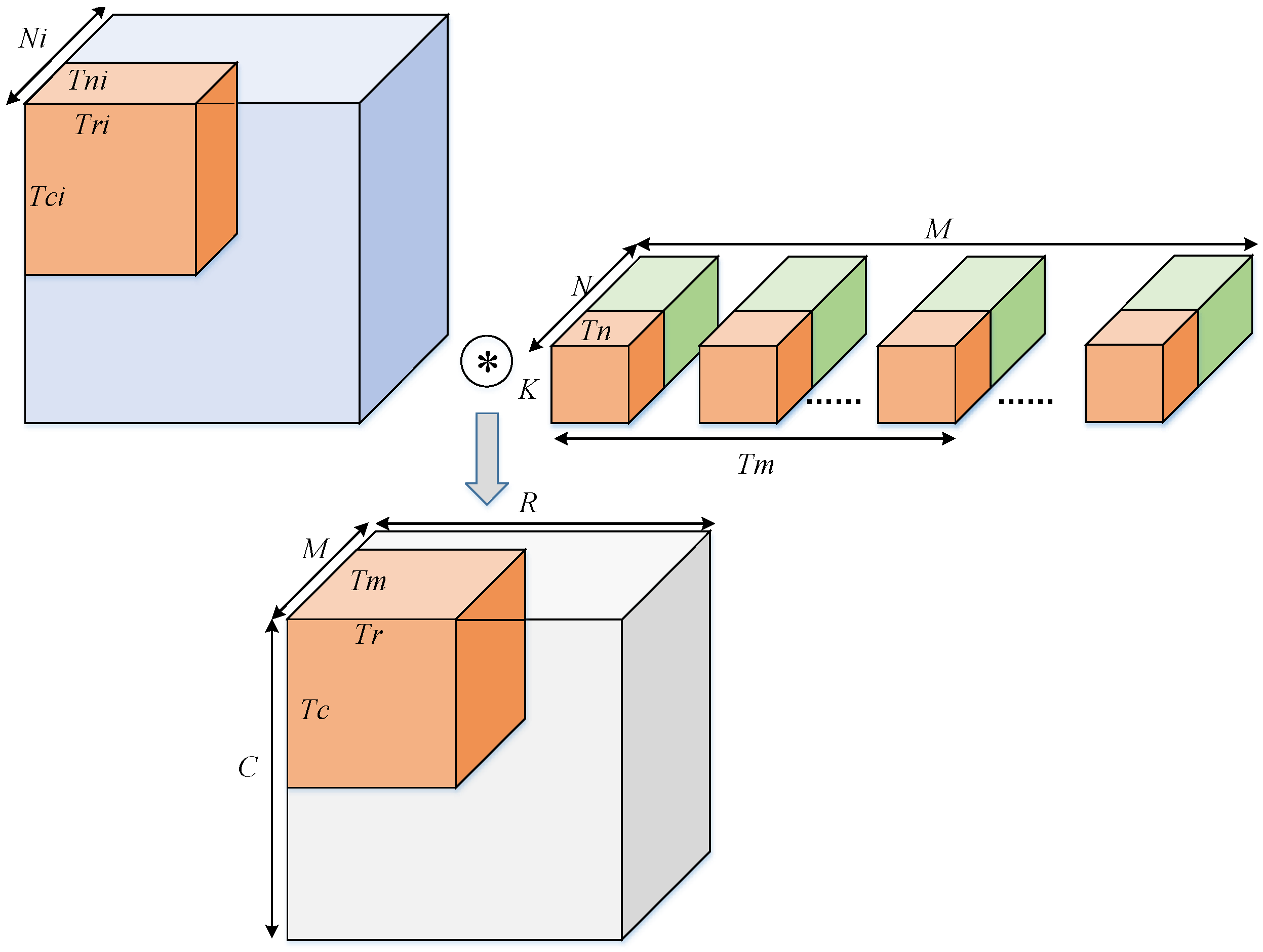
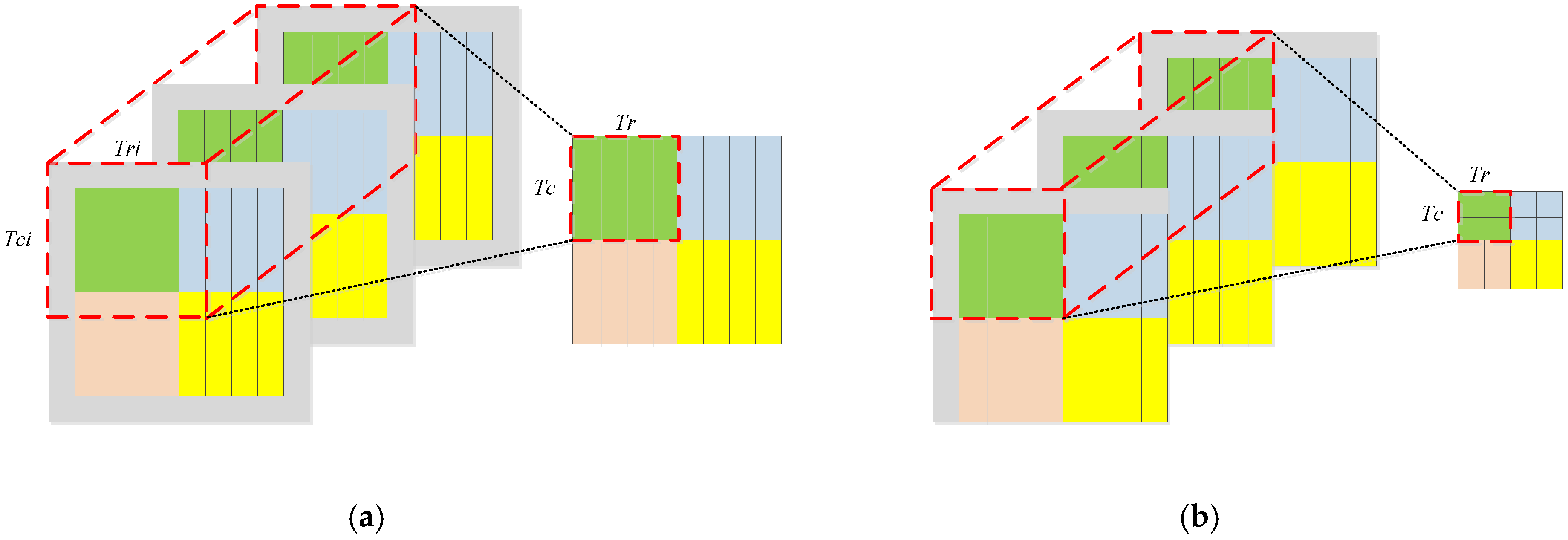
Since the on-chip cache resources are often extremely limited, this is usually unsatisfactory for all input feature maps and weights to be cached on the chip. The data must be partitioned. As shown in
Figure 7, since the convolution kernel size
itself is small, it is not divided in this dimension.
, and
are the width, height, and number of convolution kernels of the output feature map (also the number of channels of the output feature map), the channels of convolution kernel channels, and the channels of the input feature map, respectively.
,
,
, and
are the block factors of width, height of output feature map, the number and channels of convolution kernels, respectively.
,
, and
are the block factors width, height, and channels of the input feature map, respectively. The above-mentioned block coefficient setting takes into account both standard convolution and depthwise convolution.
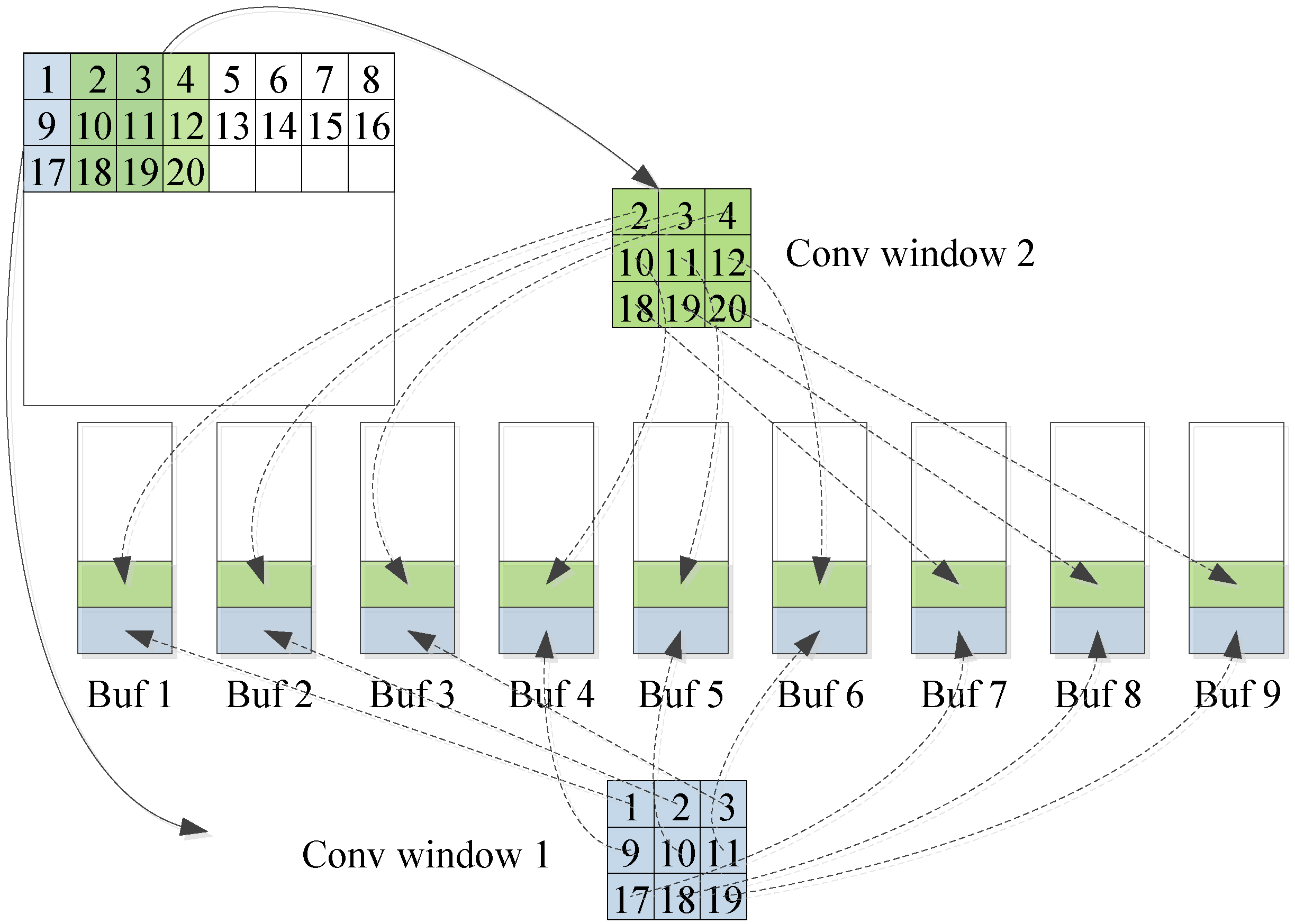
We use the example in
Figure 8 to illustrate how block convolution works. In this example, the input tensor consists of three separated channels of size 8 × 8 with additional zero padding, the kernel size is 3 × 3, and each input feature map is divided into four independent tiles. Since inter-tile dependencies are eliminated in block convolution, it is not possible to obtain an output tile of size 4 × 4 directly from three input tiles at the corresponding position. As shown in
Figure 8a, when the stride is 1, an input tile of size 6 × 6 is required to get an output tile of size 4 × 4. In
Figure 8b, an input tile of size 5 × 5 is required to get an output tile of size 2 × 2 when the stride is 2. In block convolution, the relationship between
and
can be determined as Equation (11):
Block convolution affects the external memory access of the model, which affects the
. See Equation (12), which establishes a mathematical connection between the block factors and
.
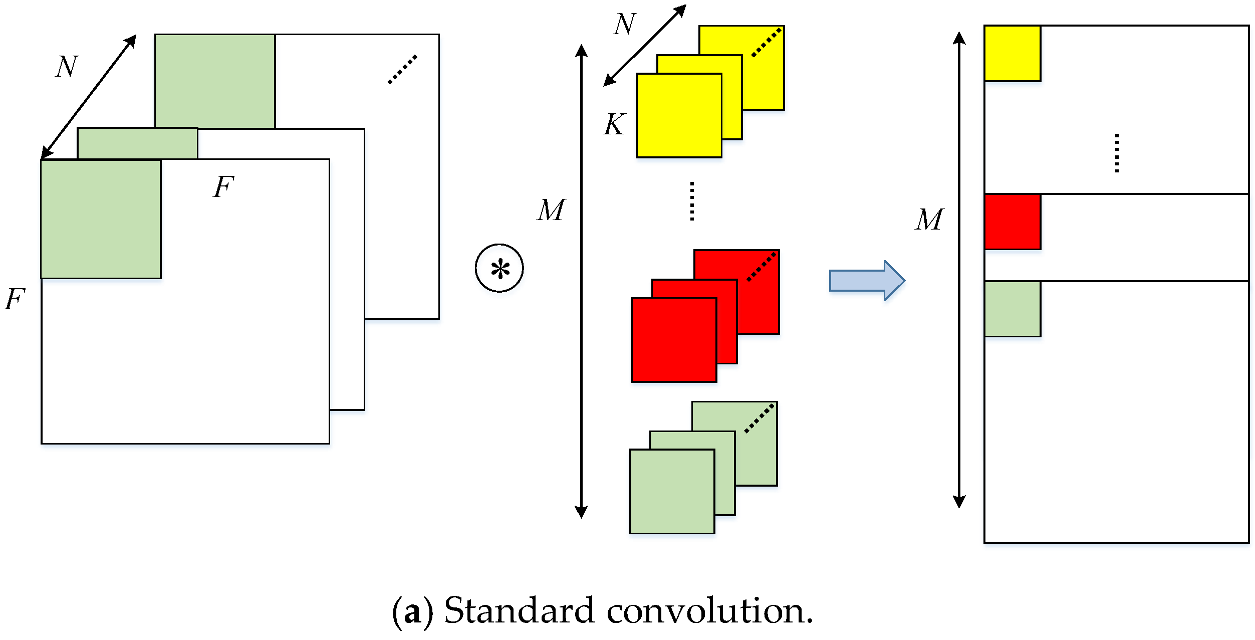
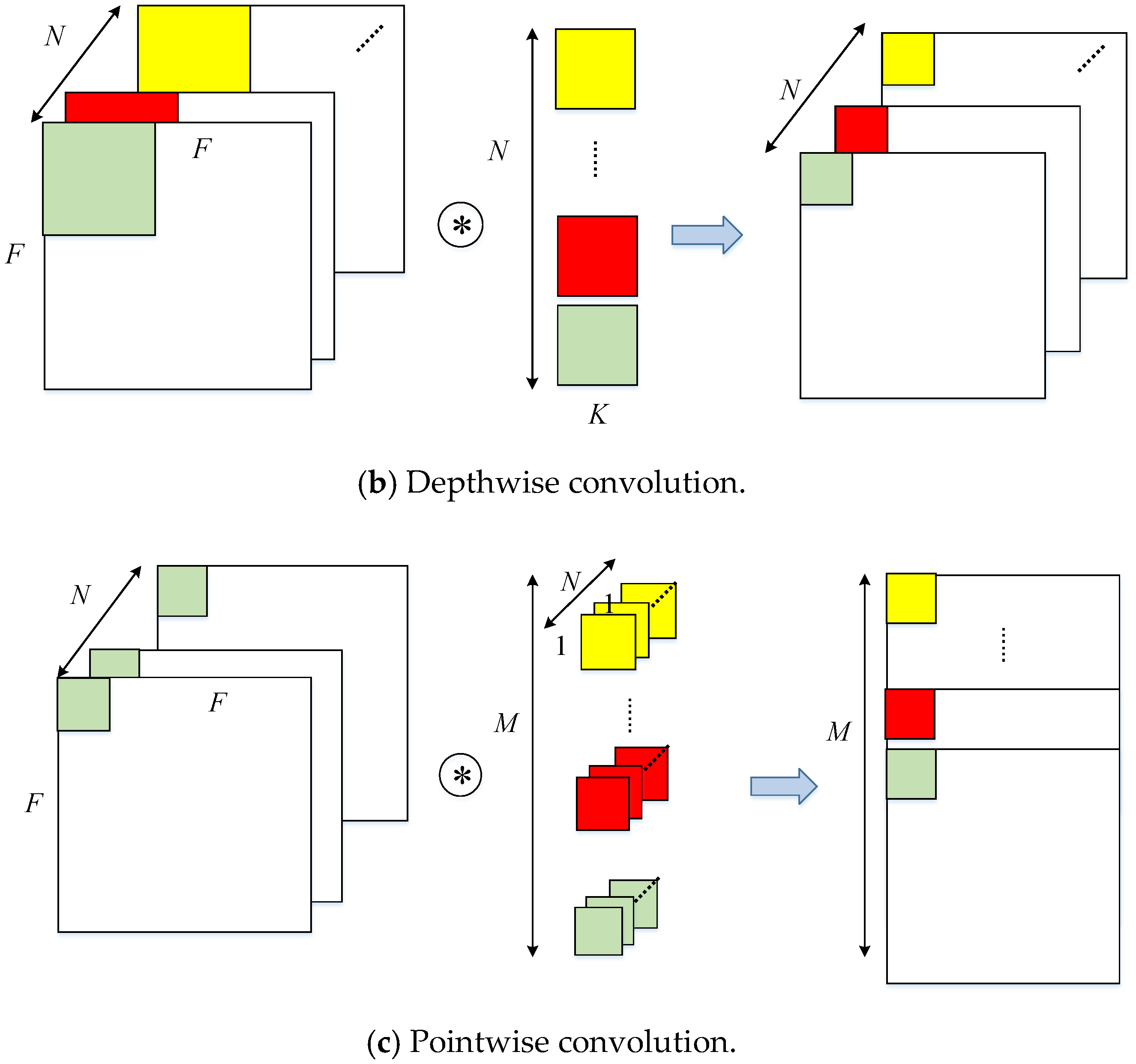
In particular, for standard convolution, and ; however, for depthwise convolution, , and .
The hardware acceleration effect of CNN depends largely on the degree of development of algorithm parallelism. CNN belongs to a feedforward multi-layer network and its interlayer structure, intra-layer operation, and data stream drive all have certain similarities. Therefore, the convolutional neural network topology CNN itself has many parallelisms. This mainly includes (1) multi-channel operation of the input feature map and convolution kernel. (2) The same convolution window and different convolution kernels can simultaneously perform convolution operations. (3) Multiple convolution windows and the same convolution kernel can simultaneously perform convolution operations. (4) In a convolution window, the parameters corresponding to all convolution kernels of all neuron nodes and corresponding parameters can be operated simultaneously. The above four parallelisms correspond to the dimensions of
,
,
, and
, respectively. Computational parallel development not only has certain requirements for computing resources, yet also requires an on-chip cache structure to provide the data needed for parallel computing. However, it also increases the on-chip cache bandwidth. The Vivado HLS development tool makes it very easy to partition an array in a particular dimension. However, if the parallelism of (3) and (4) is developed, the cache structure of the data is shown in
Figure 9.
As can be seen from the figure, if the data in a convolution window is to be distributed and stored in buffers, the data is not continuous in the dimension. Vivado HLS is difficult to implement this with array partitioning. Moreover, it repeatedly stores the overlapping data between the convolution windows which greatly increases the consumption of on-chip cache resources. Therefore, we will develop the parallelism of the calculations on the dimensions and .
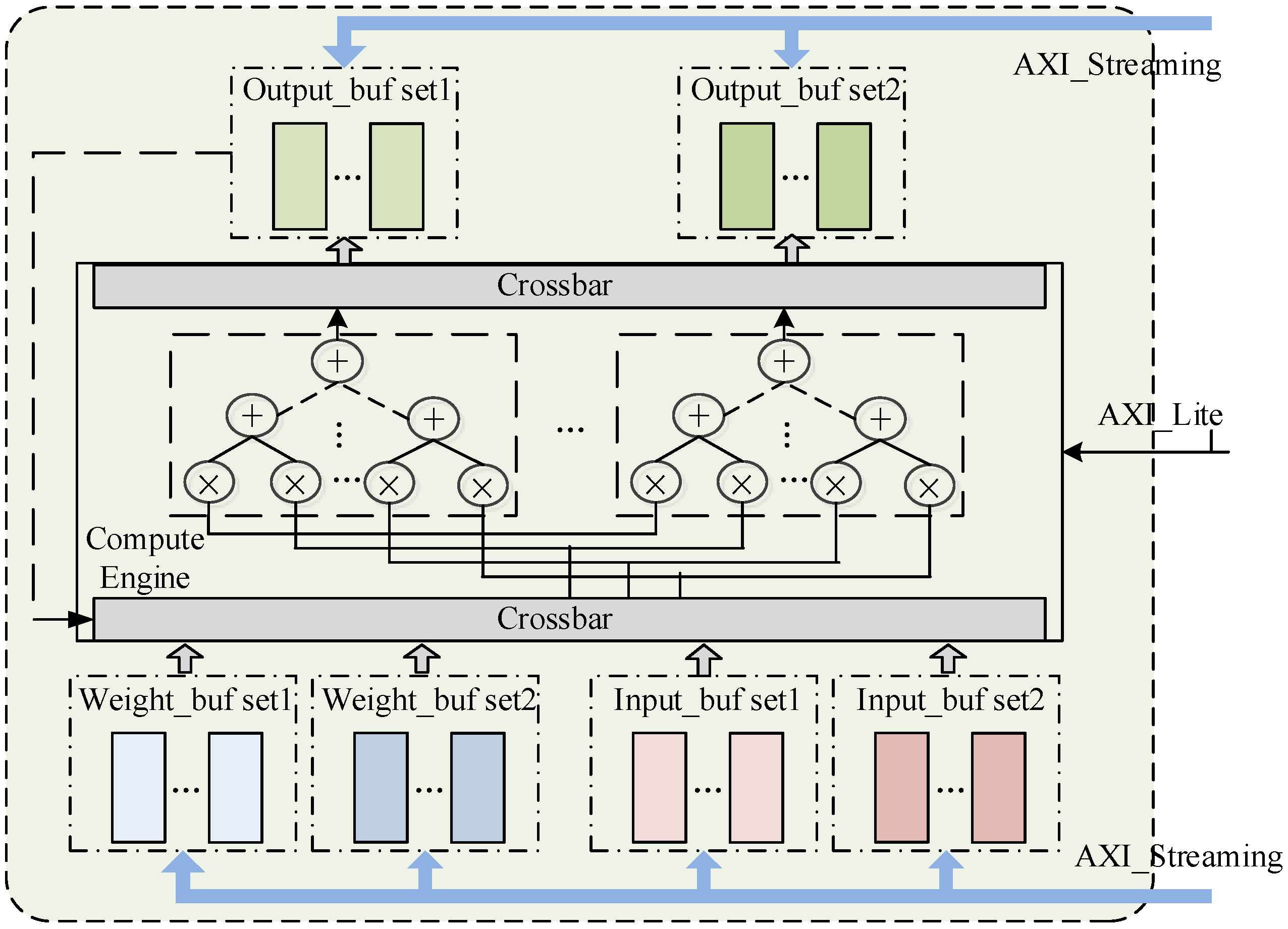
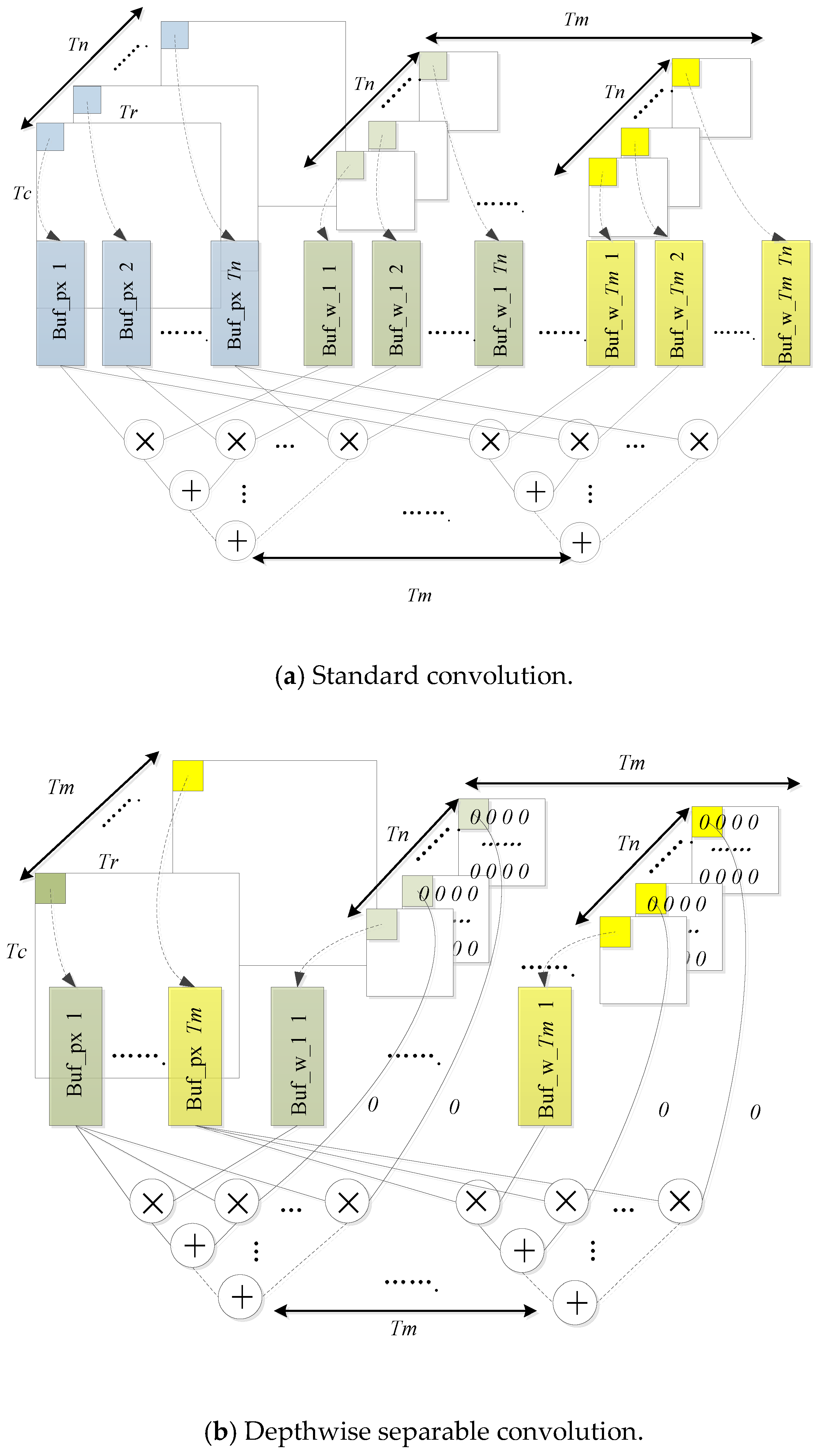
The calculation engine diagram is shown in
Figure 10. When calculating the standard convolution, the
channels of the input feature map are simultaneously multiplied by the weights of the corresponding channels and then the intermediate results are continuously accumulated which will greatly reduce the delay by pipeline. At the same time, the same operation of the
group among different convolution kernels is performed. When dealing with depthwise convolution, channels of the convolution kernel are filled with zero to
in order to efficiently integrate the two kinds of convolution and to not destroy the computational parallelism, as shown in
Figure 10b.
It can be seen from the above analysis that under the calculation engine we designed,
can be calculated by the Equation (13) for a given block factors of
,
,
, and
.
Due to array partition and ping-pong buffers, the consumption of on-chip cache resources is increased. To associate the on-chip buffer with the block factors, we need to satisfy Equation (14).
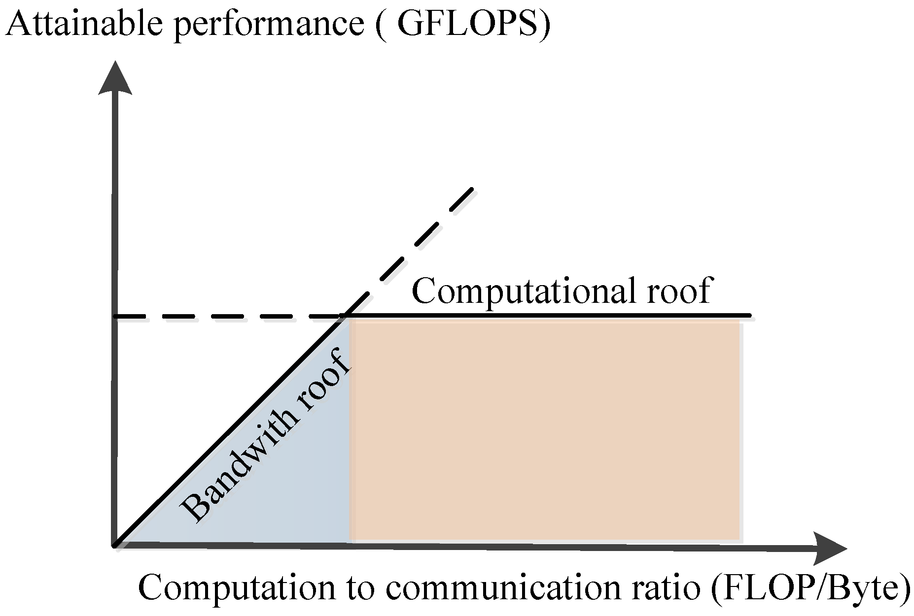
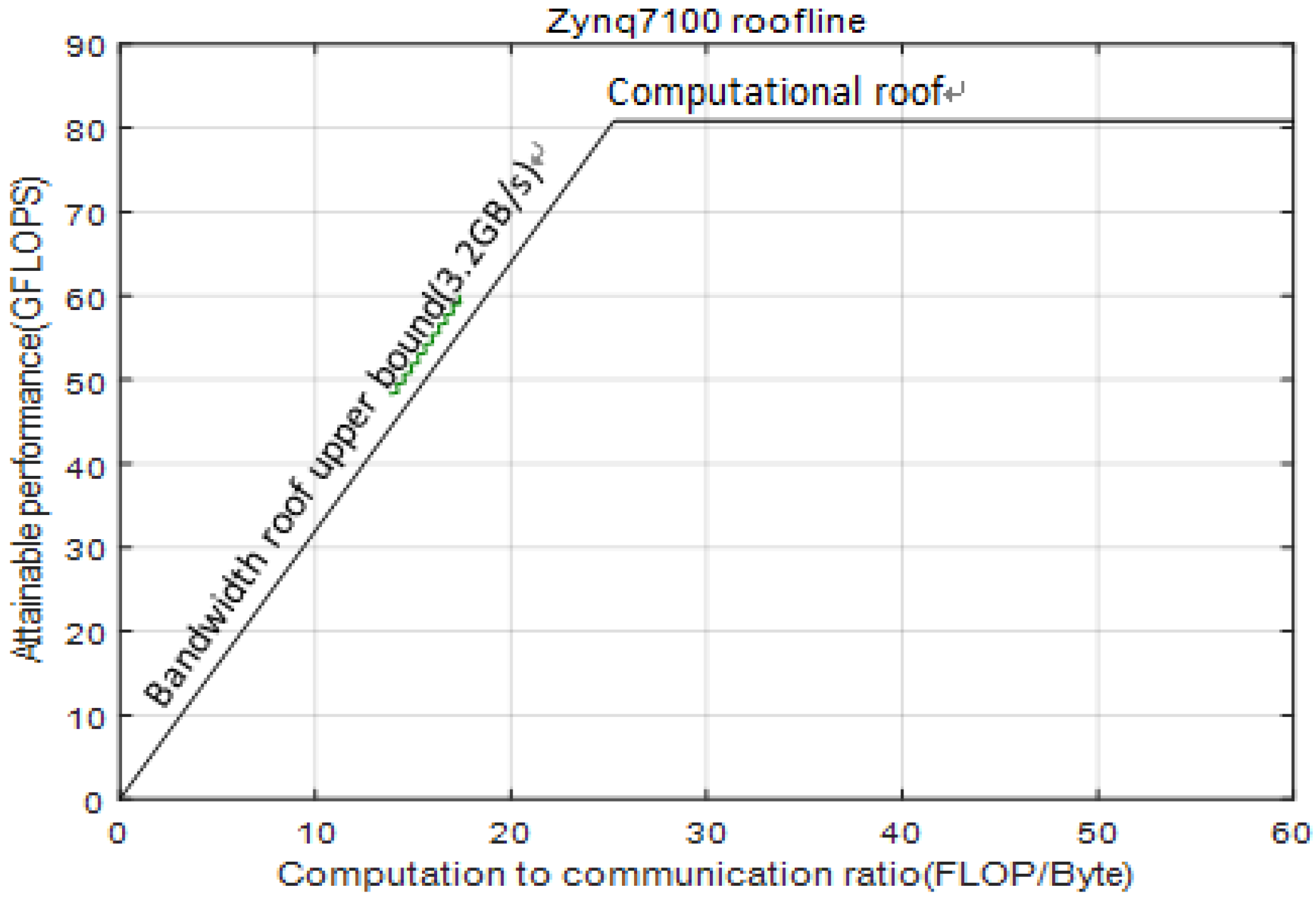
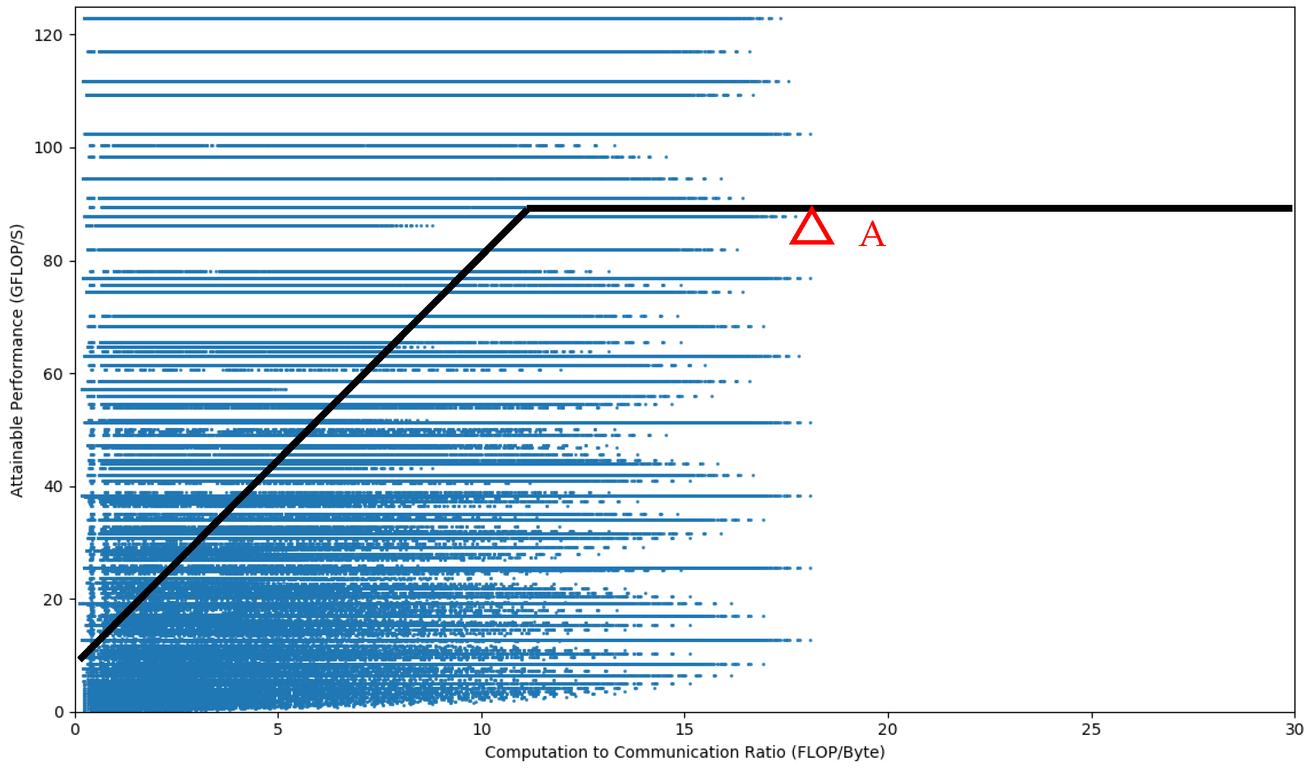
Combining the above-mentioned
,
, and the analyzed on-chip cache relationship with the roofline model of the ZYNQ 7100 under the block factors of
,
,
, and
, we seek the best design and find the optimal block factor, as shown in point A of the
Figure 11, under some certain constraints, as shown in Equation (15).
According to the above ideas, the optimal block factors
,
,
, and
of the current network layer can be obtained by programming with Matlab. However, the optimal block coefficients obtained from the different layers are different. In particular,
and
affect the computational parallelism. If
and
are allowed to be variable, complex hardware architectures need to be designed to support reconfiguration of computational engines and interconnects. So, we will solve the global optimal
and
under the whole network model, as shown in Formula (16).
where
is the number of network layers.
and
are the minimum and maximum values of
sought by all network layers.
and
are the minimum and maximum values of
sought by all network layers.
The final global optimal solution is obtained:
Since
Tn and
Tm have been determined, the configurable parameters of the accelerator are shown in
Table 1.


