Abstract
The flourishing deep learning on distributed training datasets arouses worry about data privacy. The recent work related to privacy-preserving distributed deep learning is based on the assumption that the server and any learning participant do not collude. Once they collude, the server could decrypt and get data of all learning participants. Moreover, since the private keys of all learning participants are the same, a learning participant must connect to the server via a distinct TLS/SSL secure channel to avoid leaking data to other learning participants. To fix these problems, we propose a privacy-preserving distributed deep learning scheme with the following improvements: (1) no information is leaked to the server even if any learning participant colludes with the server; (2) learning participants do not need different secure channels to communicate with the server; and (3) the deep learning model accuracy is higher. We achieve them by introducing a key transform server and using homomorphic re-encryption in asynchronous stochastic gradient descent applied to deep learning. We show that our scheme adds tolerable communication cost to the deep learning system, but achieves more security properties. The computational cost of learning participants is similar. Overall, our scheme is a more secure and more accurate deep learning scheme for distributed learning participants.
1. Introduction
1.1. Background
In recent years, artificial intelligence (AI) [1] has been applied to more and more fields, such as medical treatment [2], internet of things (IoT) [3] and industrial control [4]. Actually, deep learning [5] is one of the most attractive and representative techniques of AI, which is mainly based on neural network [6]. Thanks to the development of related computer hardware (such as GPU) and the emergence of big data [7], deep learning has achieved striking success in tasks such as image classification [8], traffic identification [9] and self-learning [10]. Therefore deep learning is gaining increasing importance in our more and more intelligent modern society.
Distributed deep learning is gaining increasing popularity nowadays. In this kind of deep learning, the training datasets are collected from multiple distributed data providers, rather than a single one [11]. When the deep learning model is trained with more representative data items, the obtained model could be more generalized, which leads to higher model accuracy. However, the collection and utilization of distributed datasets raise worrying security issues (especially privacy issues), which hinders wider application of distributed deep learning to some extent [12].
There are many examples of privacy leak, which may incur significant threats. For example, in 2018, it was reported that a data analytics company called Cambridge Analytica harvested millions of profiles of voters which revealed voters’ privacy. The data breach influenced choices of the voters which was a threat of the fairness of election. Another real live case is that the Reuters Health recently reported that some health applications in the mobile phone might share information with a host of unrelated companies, some of which have nothing to do with healthcare. A big concern of users is how their data will be used and by whom [13].
With data providers sending more and more data to cloud servers because of the cloud servers owning high computational capability and large storage to process big data, it is reasonable that data providers may worry about their data privacy, even when they encrypt their data before sending their data out [14].
Recently, Aono and Hayashi [15] presented a privacy-preserving deep learning scheme via additively homomorphic encryption. It is one of the most representative works in privacy-preserving deep learning. Their scheme is based on gradients-encrypted asynchronous stochastic gradient descent (ASGD), in combination with learning with errors (LWE)-based encryption and Paillier encryption. They first prove that sharing gradients even partially over an honest-but-curious parameter cloud server as in [16] may leak information. Then they propose an additively homomorphic encryption based scheme, in which all learning participants encrypt their own computed gradients with the same public key and send them to the server. However, the security of the scheme is based on the assumption that the server could not collude with any learning participant.
We analyze potential risks of the system in [15] as follows. (1) Since the learning participants own the same public key and private key, learning participant A could decrypt the gradients of learning participant B as long as it gets B’s encrypted gradients. (2) To make matters worse, it is likely that the server colludes with one of the participants in practice. Once the server and the learning participant collude, they could decrypt the gradients of all learning participants because the server has all encrypted gradients and the learning participant has the private key. According to [15], they could get the private local data of all learning participants through the gradients.
In our scheme, all parties (a cloud server acts as key transform server, a cloud server acts as data service provider, and data providers act as learning participants) are assumed to be honest-but-curious [17]. In other words, they will finish given tasks, but may try to mouse some sensitive information, such as the local data of data providers. We assume that the two servers, key transform server (KTS) and data service provider (DSP), are selected from different cloud companies and they would not collude with each other because of benefit contradiction (different companies take their own benefit as first consideration) and reputation preservation; however, a server may collude with a data provider.
There are two main colluding scenarios between the server and the learning participant. First, the server and a learning participant may belong to the same company. That is to say, they may collude with each other for the common benefit of their company. Specifically, the cloud company a server belongs to may send an entity to be a learning participant. But the two cloud servers are selected from different companies, so they are unlikely to collude with each other for the sake of their companies’ reputation and beneficial contradiction. Second, even if the cloud company a server belongs to cannot send an entity to be a learning participant, it is easier for a cloud sever to corrupt a learning participant than another cloud server. Because the security measures of cloud sever is more than that of a learning participant in general.
In a word, the cloud server is likely to collude with a learning participant in [15]; and it is reasonable for us to assume that the key transform server would not collude with the data service provider in this paper.
1.2. Our Contributions
Due to the security vulnerabilities of the scheme proposed in [15], we propose a multi-key based distributed deep learning scheme to protect the data privacy of learning participants even when a server colludes with one of the learning participants, using homomorphic re-encryption. We introduce a key transform server to re-encrypt the gradients encrypted by learning participants. The data service provider makes the re-encrypted gradients additively homomorphic and finishes the weights update computation. Finally, the learning participants download new weights and decrypt them respectively. The detailed realization steps of our scheme are described in Section 4. In a word, our scheme enjoys the following properties on security, efficiency and accuracy.
- Security: our scheme protects the private local data of learning participants even without the assumption that the server would not collude with any learning participant.
- Efficiency: experimental results show that the computational cost of learning participants are similar to that in [15].
- Accuracy: our scheme provides a little higher accuracy than that in [15].
1.3. More Related Works
Shokri et al. [16] have designed a distributed deep learning system that multiple learning participants could jointly train an ASGD based deep neural network model without sharing their local datasets, but must selectively sharing key parameters of the model. The goal of our paper is designing an ASGD-based distributed deep learning system which do not need sharing key parameters of the model.
Papernot et al. [18] proposed a scheme to preserve the privacy of training data called private aggregation of teacher ensembles (PATE). They used “teachers” for a “student” model instead of public models to protect sensitive data. Essentially, this property of the scheme can be called differential privacy.
NhatHai Phan et al. [19] proposed the deep private auto-encoder (dPA), which was one type of deep learning. Instead of perturbing the result of deep learning, the scheme focuses on the perturbation of objective function of the deep auto-encoder, to realize differential privacy.
Abadi et al. [20] have developed a framework of differential privacy to analyze the privacy cost of crowdsourcing the training of model over large dataset containing sensitive data. They also designed algorithmic techniques for machine learning under modest cost of privacy, computation, efficiency and accuracy.
Hitaj et al. [21] showed that distributed deep learning was susceptible to an attack they devised. They trained a generative adversarial network (GAN) generating samples that came from the same distribution as original training dataset, which should be kept private. Moreover, they showed that existing record-level differential privacy could not resist their attack. Therefore effective method is needed for privacy-preserving distributed collaborative deep learning. They consider one of the learning participants as the adversary, which is practical. We consider the situation in this paper as well.
Mohassel et al. [22] proposed privacy-preserving machine learning protocols for logistic regression, linear regression and stochastic gradient descent based neural network training. In their schemes, the data providers are distributed and there are two servers. Their schemes are based on the assumption that two servers would not collude, which is reasonable in practice because of beneficial conflict. Our system is based on this assumption, too.
Ping Li et al. [23] suggested that distributed deep learning over combined dataset should pay attention to two points. First, all data including intermediate computation results should be encrypted with different keys before being sent out. Second, the computational cost of data providers should be minimal. We fully consider these two points when we design our scheme, so that the data providers can be mobile smart phones. These authors proposed a framework for privacy-preserving outsourced classification in cloud computing (POCC) in [24].
Qingchen Zhang et al. [25] pointed out that offloading some expensive operations of big data feature learning to the cloud server(s) could improve the system efficiency. Meanwhile, the data privacy of enterprises and governments should be concerned. They approximated the activation function as a polynomial function with the Brakerski-Gentry-Vaikuntanathan cryptosystem (BGV). Our scheme do not need the approximation to avoid accuracy decrease.
BD Rouhani et al. [26] proposed a scalable provably-secure deep learning framework called Deepsecure. In this framework, all parties are likely to leak information. The key of their framework is the pre-processing techniques and optimized Yao’s Garbled Circuit protocol [27]. Our scheme considers the situation that one of the learning participants would leak information even its private key.
1.4. Paper Organization and Notations
The rest of the paper is organized as follows. We introduce the definitions of homomorphic re-encryption, ASGD-based deep learning and illustrate that gradients may leak information in Section 2, which are preliminaries of our system. The architecture of our system is proposed in Section 3. The details of realizing our system via proxy-invisible homomorphic re-encryption is given in Section 4. Then we perform security analysis of our system in Section 5. Furthermore, we analyze the communication cost of our system and evaluate its computational cost with experiments in Section 6. Finally, we conclude this paper in Section 7.
To facilitate presentation, we summarize the main notations used in this paper in Table 1.

Table 1.
Notations.
2. Preliminaries
2.1. Homomorphic Re-Encryption
Homomorphic re-encryption scheme (HRES) is an asymmetric cryptography that can realize proxy-invisible re-encryption and supports privacy-preserving data processing with access control. In addition, the addition scheme of an improved version of HRES, called the somewhat re-encryption scheme, has the properties of additive homomorphism [28]. There are four roles in this scheme: data providers (DPs), data service provider (DSP), access control server (ACS), and data requesters (DRs). As the names imply, the DPs provide data to ACS; and ACS transforms the received data to realize access control; then DSP processes the transformed data; finally, the DRs request and get data they need. Next, we introduce this improved homomorphic re-encryption scheme in detail which mainly consists of the following five algorithms.
- Key generation (KeyGen): . First choose k as a parameter, and two large primes p and q, where . The outputs of this algorithm, denoted as , are public system parameters. Determine a generator g of with maximal order [29], where is the cyclic group of quadratic residues modulo . Then compute . The two servers, DSP and access control server (ACS), respectively generate key pairs: () and (). Then they negotiate the Diffie–Hellman key:Then is published to all data providers for them to encrypt their data. Each data provider generates its own key pair. For example, the key pair of data provider i is .
- Encryption (Enc): . This algorithm is performed by data providers. Its function is encrypting plaintext () provided by data provider i under the Diffie–Hellman key . The resulting ciphertext can be represented by two parts:andwhere is first selected randomly.
- First phase of re-encryption (FPRE): . After receiving from data provider i, DSP first selects a computation identifier CID, and then implements the following algorithms to compute the intermediate ciphertext :
- Second phase of re-encryption (SPRE): . After receiving from DSP, ACS performs the following algorithms to compute :Here, the final ciphertext is obtained.
- Decryption (Dec): . Only when the data requester of has the corresponding private key , the decryption could be finished correctly. The decryption algorithms are as follows:The computation identifier CID is set to be addition here. Because only addition in HRES is used in this paper, we omit CID in the rest of this paper. According to [28], the properties of the above improved homomorphic re-encryption scheme can be summarized as follows.(1) Additive homomorphism:Because the proof of additive homomorphism property of HRES is not provided in [28] and this property is important in our scheme, we prove it in this paper as follows.Proof Proof of additive homomorphism.(2)whereandwhereBecause g is the generator with maximal order, we have , . Therefore , and HRES has the additive homomorphism property. □(3)(4) Resistant to impersonation attack and collusion between any server and any distributed data provider thanks to the two hash values . In order to avoid repetition, here we omit the proof of the last three properties. The details can be found in [28].
2.2. ASGD Based Deep Learning
Deep learning can be seen as a series of algorithms over a neural network consisting of multiple layers. There are numerous neuron nodes in each layer. The neurons of one layer are connected with neurons of next layer via weight variables. The weight variables are important for activation function which computes the output of one layer. For example, the output of layer is computed as , where is the activation function, and denotes the weight vector connecting layer p with layer .
The weight vector of the deep neural network consisting of weight variables need to be determined through deep learning. Concretely, take supervised learning for example, where a training dataset is provided firstly, and the cost function J is defined according to the target of the learning task. Then cost function is computed over all data items of the given training dataset. The learning process minimizes J by adjusting values of weight variables.
The most frequently used adjusting method called the stochastic gradient descent (SGD). Denote the weight vector as , which consists of all weights in the deep neural network. Generally, the cost function is computed iteratively over different subsets (mini-batch) of training dataset, in which elements are selected randomly. For example, the computation result of cost function over a subset consisting of t elements can be denoted as . Then the gradient vector G of cost function J can be represented as
In the learning process using SGD, the update rule for weight vector is
where is called learning rate.
In order to make the learning process more efficient, practical asynchronous stochastic gradient descent (ASGD) is proposed in [30], including data parallelism and model parallelism. Data parallelism means the training dataset for updating weight vector can be distributed. That is to say, the dataset consists of data from multiple distributed data providers. Every machine used for training model has a replica of all weights. Model parallelism is separating the model into several parts which can be updated by different machines. A typical example of model parallelism is depicted in Figure 1, which is proposed in [11]. There are learning participants included in four machines (represented by four blue rectangles with dotted lines as boundaries) in this example. The five-layer deep neural network model is separated into parts. The thick lines connecting nodes in different rectangles are called crossing weights, which are responsible for collecting different parts of models trained in different machines. The model is usually separated according to the computational capability of machines.
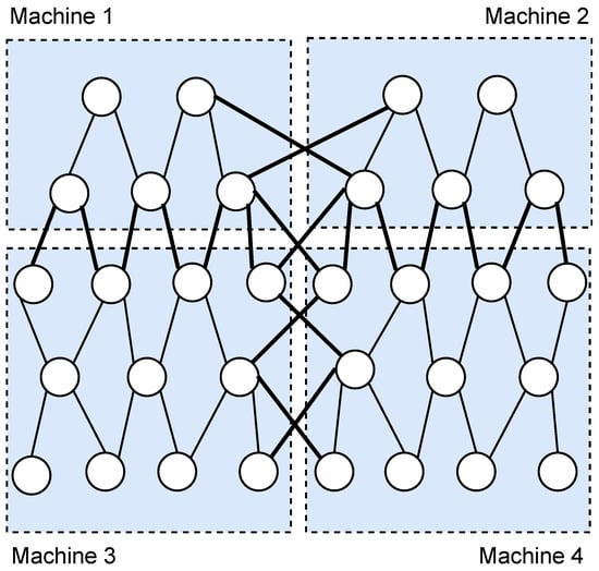
Figure 1.
An example of model parallelism.
In model parallelism, the weight variables in the deep neural network can be represented as . Each component of W, the is a weight vector. So the update rule can be transformed to
where contains the weight variables of i th part of the model updated by i th machine, means the gradient vector used for updating weights of i th part of the model, i.e., .
We adopt model parallelism in our system. The learning participant i, KTS and computing unit of DSP together act as machine i in Figure 1. Machine i is responsible for training the i th part of model assigned to it. That is to say, is updated by the local data of learning participant i. If the weight variable w connects nodes in machine i and machine k, and machine k is responsible for updating w, then the gradient used for updating w should be generated by learning participant k and should be re-encrypted with the public key of learning participant k so that machine k can further process the gradient.
2.3. Gradients Leaking Information
Authors in [15] have shown that a small portion of gradients could leak the data providers’ original training data. They proved that by listing four examples, including the simplest situation that there was only one neuron, the general neural networks, the neural networks with regularization and the most complex one, with Laplace noises added to the gradients. Here we restate the simplest example.
We focus on the learning process of one single neuron. Suppose is the data item, where is the neuron input vector and y is the corresponding truth label. The cost function here is set as the distance between the y and , is computed through the activation function f fed with
where b is the bias value. Hence the cost function is
Then the gradients can be computed as follows:
and
So the data item can be revealed by computing when the gradients are known. The truth value y can be guessed when input data item is an image according to [15].
3. System Architecture
The system architecture can be seen in Figure 2. There are three kinds of parties in our system: learning participant, KTS and DSP. The functions of them are described in detail as follows.
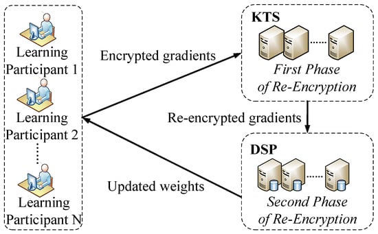
Figure 2.
System architecture.
3.1. Learning Participant
In our system, the learning participants (LPs) act as data providers, as well as data requesters. In other words, the learning participants provide the newly computed gradients for servers to update weight variables, and request the updated weight variables for next gradients generation process. Since the learning participants are distributed in our system, the training datasets are distributed as well.
To preserve the data privacy of learning participants, encrypting gradients before sending them to DSP for further processing is necessary. Different from the encryption method in [15] that all participants use one key pair generated jointly, learning participants encrypt their own gradients with the Diffie–Hellman key generated by KTS and DSP in our system. is known to all learning participants, but its corresponding private key is not overt. That is to say, any learning participant cannot decrypt the ciphertext of other learning participants to get their private data. Therefore each learning participant does not need to set up the independent secure channel to communicate with servers (KTS and DSP).
Every learning participant (suppose there are N participants) implements the following steps.
- Generate its own key pair. The public key is public to all parties of this scheme.
- Select a mini-batch of data from its own local training dataset randomly for this iteration.
- Download the encrypted weights updated in previous iteration from DSP.
- Decrypt the above encrypted weights with its own private key.
- Compute new gradients with data obtained at step 2 and weights obtained at step 4 using partial derivative.
- Encrypt new gradients with the Diffie–Hellman key and send the ciphertexts to KTS.
3.2. Key Transform Server
An innovative and important design of our system is that a KTS is responsible for parameters generation and first phase of re-encryption (FPRE). KTS mainly performs the following operations.
- Select a parameter k and two large primes randomly, where .
- Compute and choose a generator g with maximal order [29].
- Generate its key pair. Then negotiate the Diffie–Hellman key with DSP.
- Receive the ciphertexts from learning participants, and perform the FPRE over them.
- Send the re-encrypted ciphertexts to the corresponding computing unit of DSP .
3.3. Data Service Provider
Data service provider (DSP) is responsible for the second phase re-encryption and weights update. In order to make full use of the computation power of DSP and facilitate model parallelism, DSP is split into N parts which are named as computing units in our system. The steps DSP executes are as follows.
- Generate its key pair.
- Receive re-encrypted ciphertexts from KTS and perform SPRE on them.
- Update the weights using encrypted gradients obtained in step 2.
- Store the updated encrypted weights into the corresponding computing unit of DSP .
4. System Realization
In this section we use proxy-invisible homomorphic re-encryption to realize our system described in Section 3. All steps of our proposed system are listed in sequence at length as follows, which are shown in Figure 3.
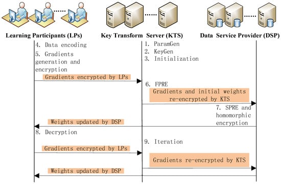
Figure 3.
System realization.
- ParamGen: . First KTS selects k as a security parameter, and two large primes p and q, where ( is the bit length of input data x). Then KTS chooses a generator g with maximal order according to [29] and computes . Finally KTS publishes the public system parameters to all entities in our system.
- KeyGen: . Every learning participant generates its own key pair .KTS and DSP generate their key pairs and respectively.Then KTS and DSP negotiate their Diffie-Hellman key . That is to say, KTS sends its public key to DSP, and DSP sends its public key to KTS. Therefore both KTS and DSP can calculate respectively.Finally, the public keys are published to all entities in our system.
- Initialization: since we adopt model parallelism, the deep neural network is separated into N parts (N is the number of learning participants). A machine (consists of a learning participant, KTS and a computing unit of DSP) is responsible for training a part of network. The weight variables in each part of the network form a weight vector respectively. So N weight vectors are assigned to N machines respectively. Before performing training process, weight vectors are initialized by KTS and shared by all parties of this system. In order to make representation clear, here we denote as the weight vector updated by Machine i in the j th weights update iteration, and is the gradient vector generated by learning participant i in the j th weights update iteration and used for updating the weight vector . The initial weight vectors are denoted as . The crossing weights connecting machine i and machine are assigned to machine k.
- Data encoding: generally, weights and gradients are real numbers. But the homomorphic re-encryption requires that numbers to be encrypted should be integers. Therefore before encrypting weights and gradients with homomorphic re-encryption, data encoding process should be performed. A real number can be represented by an integer with n bits of precision. Here we round down as the encoding result of real number x.
- Gradients generation and encryption: take the first weights update iteration for example. First, every learning participant (take the learning participant i for example here) uses a mini-batch of data selected randomly from its local dataset and the initial weight vector to calculate a gradient vector . Then calculate . Next, components of weight vector and vector are encoded into integers. Finally every learning participant encrypts components of its own vector with Diffie–Hellman key respectively and sends them to KTS. KTS encrypts each component of initial weight vector with .
- First phase of re-encryption (FPRE): After receiving the ciphertext , , …, from learning participant 1, 2, …, N respectively, KTS performs FPRE over them. Take the ciphertext received from learning participant i for example to describe the first phase of re-encryption algorithms. First KTS computes the hash value and then the re-encrypted ciphertext:Finally, KTS sends and to DSP.It is noticeable that if a gradient component is used for updating a crossing weight, then it should be re-encrypted with the public key of the learning participant the crossing weight assigned to.
- SPRE and homomorphic addition: DSP receives and from KTS and stores them in the corresponding computation unit . Each computation unit performs SPRE. Take the for example. It performs following algorithms:It is noticeable that and have the property of additive homomorphism now. So computation unit i of DSP can update the weight vectors:Finally is stored into the corresponding computation unit of DSP.
- Decryption:From the second iteration of weights update process on, each learning participant downloads updated weight vector from its corresponding computation unit of DSP. That is to say, learning participant i downloads from of DSP . Then learning participant i decrypts the downloaded with its private key . The decryption algorithms are as follows.Finally, downloaded updated by DSP is decrypted and can be used at next gradients generation iteration or deep learning model configuration when the training is finished.
- Iteration:When the training is not finished, each learning participant repeats the above step 4 to step 8 to iterate the weights update process. In other words, learning participant i computes the gradient vector with another mini-batch of data from its local dataset and . In the end of the training process, all the learning participants can get ultimate weight vector by downloading and decrypting the from the of DSP respectively.
5. Security Analysis
In this section, we present the assumption of the computational difficulty problem on which our scheme based, and then study the security of our scheme.
5.1. Assumption
Decisional Diffie-Hellman (DDH) Problem [31] over : For each probabilistic polynomial time function F, there is a negligible function so that for sufficiently large l:
That is to say, when and are given, the possibility for adversaries to distinguish between and is negligible.
5.2. Security of Our Scheme
In this section, we analyze the security of our scheme. As mentioned in Section 1.1, we consider the scenario that KTS and DSP would not collude with each other, but KTS or DSP may collude with one of learning participants. First we give the proof that our scheme is secure in the presence of semi-honest adversaries under non-colluding setting. Then we analyze the security of our system when there are colluding adversaries.
Proof.
Our scheme is secure in the presence of semi-honest adversaries under non-colluding setting. Our scheme is based on the HRES. The HRES is proved to be semantically secure in [28] based on the difficulty of Decisional Diffie–Hellman Problem above. We omit its proof here in order to avoid repetition. Our scheme involves three types of entities: LP, KTS and DSP. Three kinds of challengers are constructed to against three kinds of adversaries , who want to corrupt LP, KTS and DSP respectively.
When a new gradient G is generated, challenges as follows. First, multiplies it by and encodes the result. Then encrypts the encoded result with as . Then sends to , and outputs the entire view of : . ’s views in ideal and real executions are indistinguishable because of the security of HRES.
challenges as follows. runs encryption on two randomly chosen integers with as and . Then is multiplied by . Next performs the FPRE on the result to get , which is sent to . If responds with ⊥, returns ⊥. ’s views are made up of the encrypted data. gets the same outputs in both ideal and real executions because the LPs are honest and the HRES is proved to be secure. Therefore ’s views are indistinguishable.
challenges as follows. first chooses randomly and performs the SPRE on it with ’s private key to get . Then is sent to . If responds with ⊥, returns ⊥. ’s views are made up of the encrypted data. gets the same output in both ideal and real executions because of the security of HRES. Therefore ’s views are indistinguishable.
When it comes to decryption of the updated weight, challenges as follows. chooses randomly and decrypts it. The result is sent to . If responds with ⊥, returns ⊥. The result is the view of , which is indistinguishable in both ideal and real executions because of the security of HRES. Therefore ’s views are indistinguishable. □
Therefore our scheme is secure when there are semi-honest adversaries under non-colluding setting. Next, we illuminate that our system is secure even when KTS colludes with one of the learning participants or DSP colludes with one of the learning participants. We suppose that learning participants, KTS and DSP are honest but curious. That is to say, all parties in the system will perform the execution they should do following the system steps but they would try to get local data of learning participants. Here we analyze two situations as follows: KTS colludes with one of the learning participants, or DSP colludes with one of the learning participants.
Situation 1: KTS colludes with one of the learning participants. If KTS colludes with learning participant A, then they can share information with each other and try to get private information of other learning participants. That is to say, KTS can get the gradients of A, even the private key of A. A can get private key of KTS, too. In the scheme of [15], if the cloud server colludes with a learning participant, and the server gets the private key of the learning participant, then the server could decrypt all the gradients of all learning participants because their private keys are the same. Since the gradients leak information of original data, the private data of learning participants are not safe. However, it is impossible in our proposed scheme because all learning participants encrypt their gradients with the Diffie–Hellman key generated by KTS and DSP. KTS can not decrypt the gradients itself even with the private key of a learning participant. Because the generation of hash value can resit impersonation attack and collusion between KTS and any learning participant. KTS should perform steps in the first phase of re-encryption described in Section 4 honestly. Therefore, the private data of learning participants are secure even if KTS colludes with one of the learning participants in our scheme.
Situation 2: DSP colludes with one of the learning participants. If DSP colludes with learning participant B, the situation is similar to Situation 1. In other words, DSP can get the gradients of B, even the private key of B. B can get private key of DSP, as well as the all the re-encrypted weights and gradients. DSP should perform steps in the second phase of re-encryption described in Section 4 honestly. With the private key of learning participant B, DSP could only decrypt the gradients from learning participant B, but has no knowledge about gradients of other learning participants. Because the generation of hash value can resit impersonation attack and collusion between DSP and any learning participant. Therefore, the original data of learning participants are safe even if DSP colludes with one of the learning participants.
To sum up, our scheme is resistant to collusion between any cloud sever and any learning participant, which is not available in schemes of [15].
6. Performance Evaluation
In this section, we evaluate the communication cost and computational cost of our proposed scheme through theoretical analysis and simulation. First, we introduce the concrete parameter settings of the experiment we take.
It is shown in [28] that the length of n, influences the computation efficiency greatly, as well as security of the HRES. Experimental results showed that larger meant longer communication time, but higher security. In order to balance the efficiency and security, here we set bits, which guarantees the learning participants with limited resources can finish decryption process efficiently according to [28].
In the experiment, we generated all the private keys randomly. The influence of length of a private key on HRES was tested in [28]. From the result, we can observe that when length of private key is between 100–200 bits, the computational costs are similar. In order to compare with the scheme in [15], we set the length of private key as 128 bits in our system, which provided the same length of security parameter as that in [15].
In the data coding process, we set . That is to say, the precision of data encoding results was 32-bit. We set , which means the deep neural network was separated into 10 parts averagely and there are 10 learning participants, 10 machines and 10 weight vectors.
6.1. Communication Cost Analysis
In this section we discuss the total communication cost of our scheme . There are three kinds of communication as shown in Figure 3, communication between learning participants and KTS , communication between KTS and DSP , and communication between DSP and learning participants .
To estimate the communication cost of our scheme, first we design the following formulas:
In Equation (43), is the communication cost of iteration.
Next, we discuss the communication cost of transmitting one ciphertext between two parties. For example, ciphertext in our proposed scheme is composed of two components: , where and . The length of and are related to . Each of them has bits, so uploading or downloading one ciphertext needs to transmit bits. We set bits, so transmitting one ciphertext in our scheme means transmitting 4096 bits.
Finally, according to our system realization described in Figure 3, we can obtain the following results. For the first iteration:
For the iterations :
So the total communication cost of our scheme is
In order to compare the communication cost of our scheme with that of scheme in [15], we analyzed the increased communication factor of our scheme. The increased factor is
Since bits in our system, we can pack real numbers (after encoding into integers) into one HRES plaintext. We set the precision as bits in encoding process, and bits to prevent overflows in ciphertext additions [15]. So each ciphertext in our scheme can be used to encrypt t gradients. Therefore the increased factor is
When the number of weights update process is large enough, the increased factor of our scheme was 6. The comparison of communication cost between our scheme and latest works can be found in Table 2.
Table 2.
Communication cost comparison.
Therefore, our scheme was about six times of communication cost of the corresponding ASGD, and two times of communication cost of scheme in [15]. But in terms of learning participants, the communication cost of our scheme was similar to that in [15].
The total number of gradients in the network is 109,386 in our system. After multiplying ( is the learning rate), every gradient is encoded into a 32-bits integer and then is encrypted with . Refer to [15], we calculated the total size of ciphertext as
All the ciphertext in our system can be sent in about
via the 1 Gbps channel for communication (suppose the same communication channel speed as that in [15]).
6.2. Computational Cost Analysis
In this section we analyze the computational cost of our scheme. There are three kinds of parties in our system as shown in Figure 2, learning participants, KTS and DSP. We will analyze the computational cost of each of them respectively. We evaluate the computational cost via running time of the algorithms they execute. First we design the following formulas:
In Equation (52), is the total running time of the weights update process. When a new gradient vector (consists of many gradients generated by all learning participants) was generated, one weight’s update process began. Each learning participant encrypted their own gradients. So the computational cost of the learning participants was . Then KTS carried out the FPRE over the gradients using public keys of different learning participants respectively. So the computational cost of KTS was . Next, DSP performs SPRE over the received ciphertexts using public keys of the learning participant and updates the weights via homomorphic addition. Therefore the computational cost of DSP was . Finally, learning participants download and decrypt the updated weights using their own private keys respectively. Hence, the computational cost of learning participants was .
Next, we estimated the computational cost of our scheme through simulations. In order to compare the computational cost of our scheme with that of the LWE-based scheme in [15], we used the Tensorflow 1.8.0 library and Cuda-9.0 to construct the same fully connected multilayer perceptron (MLP) network as that in [15], with four layers (784-128-64-10 neurons sequentially). The total number of gradients in the network is 109,386 as well. The detailed experimental settings in model training are shown in Table 3.
Table 3.
Experimental settings in model training.
We implement our scheme with C++ codes. The network and scheme are run on a computer with NVIDIA GeForce GTX 1080 Ti, Intel(R) Core(TM) I7-4702MQ CPU @ 2.20 GHz and 16 G Memory. The operating system is Windows 10.
According to simulation, the average running time of gradients generation process through training the MLP in our scheme was ms; and the HRES running time of processing the 109,386 gradients of the network with 10 learning participants in one weights update process was ms. Therefore, the running time of one weights update process in our system was
The average running time per weights update iteration for performing steps of homomorphic re-encryption in our scheme, including encryption, FPRE, SPRE, homomorphic addition and decryption time are depicted in Figure 4, which are denoted as encTime, FPRETime, SPRETime, addTime and DecTime respectively.
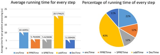
Figure 4.
(a) Average running time for every step. (b) Percentage of running time for every step.
As mentioned above, learning participants were responsible for the implementation of encryption and decryption; KTS was responsible for FPRE; DSP was responsible for SPRE and addition. So we calculated the computational cost of them respectively in Table 4 (accurate to the second decimal place). It can be seen that DSP had the maximum computational overhead (). The computational cost of learning participants are of the total computational cost. There were 10 learning participants in our system, and we separated the model averagely, so the average computational cost of every learning participant was just , which was much lower than that of KTS and DSP. The configuration was reasonable because the computational capability of cloud server is much higher than that of every data provider generally.
Table 4.
Average computational cost of parties in our scheme.
The experimental results comparison is shown in Figure 5 and Table 5. In Figure 5, of our scheme consists of there parts: running time of encryption, FPRE and SPRE. In Table 5, means the running time of using our scheme to process the gradients and update the weights. It consists of five parts in our scheme: encryption (1112.4 ms) and decryption (584.1 ms) by learning participants, FPRE (630.2 ms) by KTS, SPRE (615.1 ms) and homomorphic addition (2250.6 ms) by DSP. On the other hand, the LWE-MLP scheme in [15], consists of there parts: encryption (899.2 ms) and decryption (785.4 ms) by learning participants, homomorphic addition (278.9 ms) by DSP.
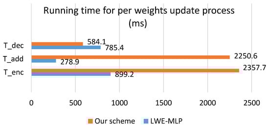
Figure 5.
Experimental results comparison.
Table 5.
Experimental results comparison.
The running time of our system was about 2.64 times of that in LWE-MLP [15]. Although the total running time of our system was longer, the computational cost of learning participants was similar to that of [15], which is shown in Table 6. The accuracy is , which was a little higher than that in [15].
Table 6.
Computational cost of parties comparison.
7. Conclusions
Considering that previous distributed deep learning scheme sharing single key pair for encryption suffers from collusion between cloud server and any learning participant [15], we propose a novel system using homomorphic re-encryption which makes privacy-preserving distributed deep learning come true. We give the detailed realization steps of our system and implement them for validation. Furthermore, security analysis and performance evaluation are provided. Specifically, the communication cost of our scheme is tolerable. Experimental results show that although the running time of our system is larger than that of LWE-MLP in [15], but the computational overhead of learning participants is nearly the same as that in [15]. More importantly, our system is more secure and accurate because it is collusion-resistant between any server and any learning participant, with higher deep learning accuracy.
Author Contributions
F.T. contributed to writing—original draft preparation, methodology, software and validation of the proposed scheme; W.W. contributed to conceptualization; J.L. contributed to writing—review and editing and funding acquisition; H.W. contributed to supervision; and M.X. contributed to project administration.
Funding
This research was funded by the National Natural Science Foundation of China under Grant No. 61801489.
Conflicts of Interest
The authors declare no conflict of interest. The funders had no role in the design of the study; in the collection, analyses, or interpretation of data; in the writing of the manuscript, or in the decision to publish the results.
Abbreviations
The following abbreviations are used in this manuscript:
| LP | Learning participant |
| KTS | Key transform server |
| DSP | Data service provider |
| LWE-MLP | Learning with error-multilayer perception |
References
- Russell, S.J.; Norvig, P. Artificial Intelligence: A Modern Approach; Pearson Education Limited: Harlow, UK, 2016. [Google Scholar]
- Bennett, C.C.; Hauser, K. Artificial intelligence framework for simulating clinical decision-making: A Markov decision process approach. Artif. Intell. Med. 2013, 57, 9–19. [Google Scholar] [CrossRef] [PubMed]
- Marjani, M.; Nasaruddin, F.; Gani, A.; Karim, A.; Hashem, I.A.T.; Siddiqa, A.; Yaqoob, I. Big IoT data analytics: Architecture, opportunities, and open research challenges. IEEE Access 2017, 5, 5247–5261. [Google Scholar]
- Jamal, A.; Syahputra, R. Heat Exchanger Control Based on Artificial Intelligence Approach. Int. J. Appl. Eng. Res. (IJAER) 2016, 11, 9063–9069. [Google Scholar]
- LeCun, Y.; Bengio, Y.; Hinton, G. Deep learning. Nature 2015, 521, 436. [Google Scholar] [CrossRef] [PubMed]
- Schmidhuber, J. Deep learning in neural networks: An overview. Neural Netw. 2015, 61, 85–117. [Google Scholar] [CrossRef] [PubMed]
- Mayer-Schönberger, V.; Cukier, K. Big Data: A Revolution That Will Transform How We Live, Work, And Think; Houghton Mifflin Harcourt: Boston, MA, USA, 2013. [Google Scholar]
- Zhong, P.; Gong, Z.; Li, S.; Schönlieb, C.B. Learning to diversify deep belief networks for hyperspectral image classification. IEEE Trans. Geosci. Remote Sens. 2017, 55, 3516–3530. [Google Scholar] [CrossRef]
- Wang, Z. The applications of deep learning on traffic identification. BlackHat USA 2015. Available online: https://www.blackhat.com/docs/us-15/materials/us-15-Wang-The-Applications-Of-Deep-Learning-On-Traffic-Identification-wp.pdf (accessed on 8 April 2019).
- Zhang, L.; Gopalakrishnan, V.; Lu, L.; Summers, R.M.; Moss, J.; Yao, J. Self-learning to detect and segment cysts in lung CT images without manual annotation. In Proceedings of the 2018 IEEE 15th International Symposium on Biomedical Imaging (ISBI 2018), Washington, DC, USA, 4–7 April 2018; pp. 1100–1103. [Google Scholar]
- Dean, J.; Corrado, G.; Monga, R.; Chen, K.; Devin, M.; Mao, M.; Senior, A.; Tucker, P.; Yang, K.; Le, Q.V.; et al. Large scale distributed deep networks. In Proceedings of the Advances in Neural Information Processing Systems, Lake Tahoe, ND, USA, 3–6 December 2012; pp. 1223–1231. [Google Scholar]
- Liang, Y.; Cai, Z.; Yu, J.; Han, Q.; Li, Y. Deep learning based inference of private information using embedded sensors in smart devices. IEEE Netw. 2018, 32, 8–14. [Google Scholar] [CrossRef]
- Hao, J.; Huang, C.; Ni, J.; Rong, H.; Xian, M.; Shen, X.S. Fine-grained data access control with attribute-hiding policy for cloud-based IoT. Comput. Netw. 2019, 153, 1–10. [Google Scholar] [CrossRef]
- Wu, W.; Parampalli, U.; Liu, J.; Xian, M. Privacy preserving k-nearest neighbor classification over encrypted database in outsourced cloud environments. World Wide Web 2019, 22, 101–123. [Google Scholar] [CrossRef]
- Phong, L.T.; Aono, Y.; Hayashi, T.; Wang, L.; Moriai, S. Privacy-preserving deep learning via additively homomorphic encryption. IEEE Trans. Inf. Forensics Secur. 2018, 13, 1333–1345. [Google Scholar]
- Shokri, R.; Shmatikov, V. Privacy-preserving deep learning. In Proceedings of the 22nd ACM SIGSAC Conference on Computer And Communications Security, Denver, CO, USA, 12–16 October 2015; ACM: New York, NY, USA, 2015; pp. 1310–1321. [Google Scholar]
- Chai, Q.; Gong, G. Verifiable symmetric searchable encryption for semi-honest-but-curious cloud servers. In Proceedings of the 2012 IEEE International Conference on Communications (ICC), Ottawa, ON, Canada, 10–15 June 2012; pp. 917–922. [Google Scholar]
- Papernot, N.; Abadi, M.; Erlingsson, U.; Goodfellow, I.; Talwar, K. Semi-supervised knowledge transfer for deep learning from private training data. arXiv, 2016; arXiv:1610.05755. [Google Scholar]
- Phan, N.; Wang, Y.; Wu, X.; Dou, D. Differential Privacy Preservation for Deep Auto-Encoders: An Application of Human Behavior Prediction. In Proceedings of the Thirtieth AAAI Conference on Artificial Intelligence, Phoenix, AZ, USA, 12–17 February 2016; Volume 16, pp. 1309–1316. [Google Scholar]
- Abadi, M.; Chu, A.; Goodfellow, I.; McMahan, H.B.; Mironov, I.; Talwar, K.; Zhang, L. Deep learning with differential privacy. In Proceedings of the 2016 ACM SIGSAC Conference on Computer and Communications Security, Vienna, Austria, 24–28 October 2016; ACM: New York, NY, USA, 2016; pp. 308–318. [Google Scholar]
- Hitaj, B.; Ateniese, G.; Perez-Cruz, F. Deep models under the GAN: Information leakage from collaborative deep learning. In Proceedings of the 2017 ACM SIGSAC Conference on Computer and Communications Security, Dallas, TX, USA, 30 October–3 November 2017; ACM: New York, NY, USA, 2017; pp. 603–618. [Google Scholar]
- Mohassel, P.; Zhang, Y. SecureML: A system for scalable privacy-preserving machine learning. In Proceedings of the 2017 38th IEEE Symposium on Security and Privacy (SP). IEEE, San Jose, CA, USA, 22–24 May 2017; pp. 19–38. [Google Scholar]
- Li, P.; Li, J.; Huang, Z.; Li, T.; Gao, C.Z.; Yiu, S.M.; Chen, K. Multi-key privacy-preserving deep learning in cloud computing. Future Gener. Comput. Syst. 2017, 74, 76–85. [Google Scholar] [CrossRef]
- Li, P.; Li, J.; Huang, Z.; Gao, C.Z.; Chen, W.B.; Chen, K. Privacy-preserving outsourced classification in cloud computing. Cluster Comput. 2018, 21, 277–286. [Google Scholar] [CrossRef]
- Zhang, Q.; Yang, L.T.; Chen, Z. Privacy preserving deep computation model on cloud for big data feature learning. IEEE Trans. Comput. 2016, 65, 1351–1362. [Google Scholar] [CrossRef]
- Rouhani, B.D.; Riazi, M.S.; Koushanfar, F. Deepsecure: Scalable provably-secure deep learning. In Proceedings of the 2018 55th ACM/ESDA/IEEE Design Automation Conference (DAC), San Francisco, CA, USA, 24–28 June 2018; pp. 1–6. [Google Scholar]
- Kiraz, M.; Schoenmakers, B. A protocol issue for the malicious case of Yao’s garbled circuit construction. In Proceedings of the 27th Symposium on Information Theory in the Benelux, Louvain-la-Neuve, Belgium, 19–20 May 2006; pp. 283–290. [Google Scholar]
- Ding, W.; Yan, Z.; Deng, R.H. Encrypted data processing with homomorphic re-encryption. Inf. Sci. 2017, 409, 35–55. [Google Scholar] [CrossRef]
- Ateniese, G.; Fu, K.; Green, M.; Hohenberger, S. Improved proxy re-encryption schemes with applications to secure distributed storage. ACM Trans. Inf. Syst. Secur. (TISSEC) 2006, 9, 1–30. [Google Scholar] [CrossRef]
- Recht, B.; Re, C.; Wright, S.; Niu, F. Hogwild: A lock-free approach to parallelizing stochastic gradient descent. In Proceedings of the Advances in Neural Information Processing Systems, Granada, Spain, 12–14 December 2011; pp. 693–701. [Google Scholar]
- Boneh, D. The decision diffie-hellman problem. In Proceedings of the International Algorithmic Number Theory Symposium, Portland, OR, USA, 21–25 June 1998; Springer: Berlin, Germany, 1998; pp. 48–63. [Google Scholar]


© 2019 by the authors. Licensee MDPI, Basel, Switzerland. This article is an open access article distributed under the terms and conditions of the Creative Commons Attribution (CC BY) license (http://creativecommons.org/licenses/by/4.0/).