A company has an active connection to the smart meter where the HAN network provides the proposed load scheduling system with access to each device. For each time slot the total load will be denoted as . For a given customer, the set of household appliances will be referred to as and these devices include items such as a washing machine, stove, refrigerator or any connected device. For a given appliance e, the one-slot energy consumption scheduled at time slot t is referred to as . The first objective of the multi-objective functions of the MODE algorithm is the cost of energy that is consumed by the household. In the meantime, the peak of the load is considered the second objective. The goal of the MODE algorithm is to schedule the load to save energy cost and peak concurrently.
2.1. Multi-Objective Optimization Differential Evolution (MODE)
In general, evolutionary algorithms (EAs) are being utilized to solve optimization problems with multi-objectives that are traced back to its ability to process a number of solutions and yields an optimal Pareto front with fast convergence and high diversity [
31]. The MODE algorithm model is mainly based on a conventional differential evolution algorithm that can resolve multi-objective optimization (MOO) problems. For this research, the MODE algorithm has been utilized to optimize the starting time of 10 operative appliances as a bi-objective real optimization problem. To optimize the load scheduling problem, the cost and peak load have been utilized as the two objectives. In general, the main significance of MOO algorithms is to offer a set of ideal solutions, as denoted by the Pareto front [
32,
33]. In addition, in the selection stage of single-objective optimization algorithms, the parent solution is exchanged for the candidate (child) solution when the last one is better than the parent solution in terms of objective function. Meanwhile, in MOO algorithms, the replacement’s decision is not straightforward like a single-objective optimization algorithm because there are many objective functions that dominate the problem. The Pareto optimality (dominance) principle can be considered one of the most rigid techniques that are adapted to realize the replacement between the parent and child solutions in the selection stage. The details of the MODE model are depicted by the following algorithm.
Step 1: The first phase of MODE is creating an initial population set with
individual vectors and
decision variables as follows:
where,
is the target vector and
is an index which points to the counts of generation (
,
are two indices, which refer to the number of individual vectors (solutions) and number of decision variables that comprises each solution, respectively. Here, the initial values of
elements of each individual vector are randomly chosen and uniformly distributed in the search space. Furthermore, the search space is bounded by the upper (
and lower (
bounds. The elements of the initial individual vector are selected as below,
where
is a pseudo-random number that is generated by using a uniform distribution and belongs to the interval (0, 1). After that, the corresponding objective functions to current target vector are computed and saved in vectors to use them in the next steps.
Step 2: The mutant vector is generated in MODE by adding the third individual vector with the weighted difference between two individual vectors [
34]. Therefore, a mutant vector
for any individual vector
, is generated as below:
where,
vectors are selected in a random fashion from the population set and they are not equal to the current individual vector
. The values of
are indices that have values in the range of [1,
]. The base vector here is defined as
while the mutation scaling factor is indicated as
, which is basically picked up within the interval [0, 1] [
35].
Step 3: Within the next step of the MODE algorithm, the trial vector
is generated by using the mutant vector
and the target vector
. In this step, two numbers are randomly selected to dominate the selection process between the mutant and the target vectors. The first one,
is randomly belongs to (0, 1) interval, while the second one is
, which is chosen in a random fashion from the interval that is in the range [1,
]. The trial vector equals to the mutant vector if the
number is less than or equal to the crossover control factor (
) or the value of
equals to the current index (
) that refers to the decision variable. Otherwise, the trial vector equals to the corresponding target vector and the mutant vector is neglected. It is worth to mention that the
is selected in a random fashion in the range of
[
35].
Step 4: The elements of the trial vector must be analysed to determine whether these elements are within the permitted search space or not and to validate that these are realistic values. If any element is outside the allowed limits of the search space, then the element is exchanged with a new element, which is computed using Equation (5).
Step 5: The last step of the MODE algorithm is the selection step, which is applied after generating
child solutions. The selection process between the child solution (
) and the current parent solution (
) is started by creating a temporary population (
). The individual vectors of the temporary population are chosen from both
and
.
is rejected from
if
is dominated by the corresponding
and vice versa. Under other conditions, each of
and
are expressed as an element of
once the child and parent solutions are not dominating each other. Temporary population’s size is usually expected between
and
. Accordingly, the temporary population’s size is minimized to reach the value of
solutions so as to prepare it for the next generation. The size of reduction depends on the next two sub steps [
36]:
Step 5.1: In this sub step, the solution of temporary population is classified into many front levels (
[
37,
38]. The first front level
is made up from solutions that are non-dominated by other solutions and these solutions are ranked as 1. The solutions are non-dominated by other solutions except by the ones that belong to front level
, which are ranked as 2 to form the second front level
and so on. Meanwhile, solutions dominated only by other solutions belong to the front levels
will be ranked as
K with
front level. Upon the completion of a non-dominated sorting algorithm, the newest population which has been arranged for the next generation is to combine different solutions that apply to various non-dominated front levels. To fill the new population, the non-dominated front level solution of rank 1 is chosen first. Then, it is tracked by solutions that belong to front levels 2, 3 and so on. Since the temporary population’s size is within the range [
,
], then not all
solutions must be included in the new population’s
slots. Solutions that have been eliminated in the population of the next generation are excluded. A related point to consider is solutions that belong to the last allowable rank can be larger than other slots remained in the next generation’s population. With such scenario, in order to choose solutions that lie in the least crowded region, a crowding distance ranking model is utilized. This will in turn increase solutions’ diversity instead of arbitrarily discarding some solutions.
Step 5.2: In the MODE algorithm, the diversity of optimal solutions is increased by applying the crowding distance rank principle that presented in non-dominated sorting genetic algorithm-II [
39]. The solutions’ density surrounding a solution
can be estimated by computing along each objective the average distance which corresponds with two solutions on the right and left sides of a solution
. Thus, the circumference of a rectangle with the right and left vertices of neighbor solutions is said to be the crowding distance of any given solution
. The best solutions are the ones that have a high crowding distance rank, since these solutions offer much diversity in the population [
37]. Along
zth objective function, a crowding distance of
ith solution is calculated as:
where
refers to the value of a single crowding distance of the
ith solution that relates to
zth objective function.
is
zth objective function for
solution and
is
zth objective function for
solution. In addition,
is the minimum and
is the maximum values of the
zth objective function. In the meantime, by obtaining the summation value of all individual crowding distances along each objective, the total value of a crowding distance of every solution can be determined and is represented as follows:
The model that is applied to calculate the crowding distance rank for every solution belongs to an
ith front level (
) with bi-fitness functions is illustrated in the pseudo code of MODE model (
Appendix A), which is proposed to optimize the starting time of operating electrical devices with minimum cost and load peak.
2.2. Hybrid AHP-TOPSIS Model Load Scheduling
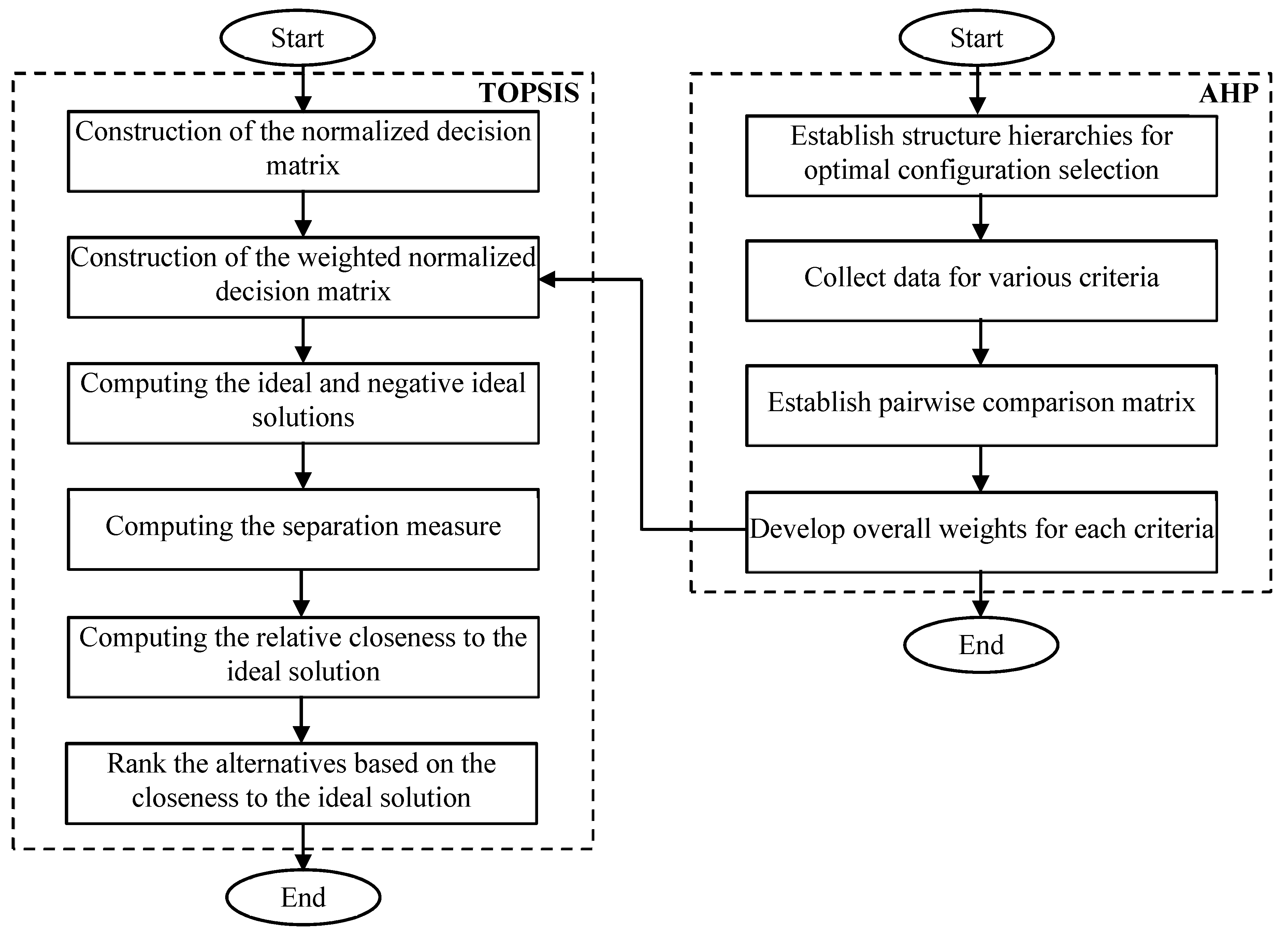
In this work, an AHP-TOPSIS model is utilized to sort the optimal solutions’ set of load scheduling system that obtained by the MODE algorithm and ranked from the best solution to the
appropriate weights for each criterion according to the evaluation of evaluators (expert). For the second, the TOPSIS approach has been utilized with predefined weights, in order to sort the solutions of the problem. The proposed hybrid AHP-TOPSIS model that obtains the optimal set of time operation of customer load is depicted in
Figure 1. The details of the proposed model will be discussed in the following subsection.
2.2.1. AHP Approach for Deriving Weights of Criteria
Each criterion has a degree of importance to dominate the performance of the MCDM problem. The degree of importance can be presented by weight value, where the weight’s sum of total criteria of the MCDM problem must be controlled by
where
is the entire criteria’s count that dominates the MCDM problem and
is the weight of
jth criteria. Saaty in 1977 [
40] proposed the AHP model to derive the appropriate weights for each criteria in the MCDM problem. The AHP method depends on the comparisons between a pairwise criteria. However, the total number of pairwise comparisons for
-criteria problem is
. The pairwise comparison is achieved by using the Saaty scale which was presented by Saaty [
41]. The Saaty scale comprises nine preference points to enable the evaluator to specify the number of times a single criterion is more or less important than another. A questioner which depends on the expertise of three experts (evaluators) is realized to accomplish a comparison between a pairwise criteria of MCDM problem. The evaluations of experts are tabulated in
Table 1,
Table 2 and
Table 3. The preference of evaluators is done as three steps whereas, the first evaluator does not give preference for each criterion. In the meanwhile, the second and third evaluators are strong and slightly favour the cost criterion over the peak criterion, respectively.
According to the evaluator preferences,
Table 4 depicts the construction of a comparison matrix. The comparison matrix is normalized by dividing each element belongs to a column by the sum of the column’s elements. After that, the elements of each row of the normalized matrix are aggregated and finally divided by the sum of them to acquire weights of each criteria.
2.2.2. Technique for Order Preferences by Similarity to Ideal Solution (TOPSIS)
Yoon and Hwang proposed TOPSIS in 1980 to solve multi-dimensional MCDM problems [
30]. In this method, the shortest and fastest distances from the negative ideal and ideal solutions play an important role in sorting the alternatives. For simplicity, the MCDM problem may be presented in a matrix with
alternatives and
criteria which have variables weight (
, where
) that have been previously derived by the AHP method. The decision matrix (
DM) that represents the MCDM (Equation (11)) comprises of the performance (
) of
ith alternative (
) in terms of
jth criteria (
), where
and
. The TOPSIS technique can be expressed according to the next steps:
Step 1: Constructing normalized decision matrix:
In general, DM’s criteria differ in measuring units (multi-dimension criteria). Therefore, the elements of DM should be normalized using the following formula.
Accordingly, normalized decision matrix () can be defined as
Step 2: Constructing normalized weighted decision matrix:
The normalized weighted decision matrix () is constituted by utilizing the normalized decision matrix () with weights that have been acquired through AHP model. The elements of are computed by multiplying the elements of by the corresponding weight as given by;
Thus, the obtained matrix from step 2 can be described by
Step 3: Calculating the negative ideal and ideal solutions:
In steps 3, ideal (
) and negative (
) solutions are computed as follow
where
is a set of benefit criteria with period [1,
] and
is the complement set of
with period [1,
], which refers to the cost criterion. Above all, the most preferable solution (alternative) is the ideal solution (
). On the other hand, the least preferable solution is the negative ideal solution (
).
Step 4: Separation measure’s calculation process:
In this step, the
-dimension Euclidean distance has been utilized to calculate the separation distance between each alternative in matrix
and the negative ideal and ideal solutions. Where the distance (
) of an alternative (
) from the ideal solution (
) can be indicated by
Similarly, the distance () between an alternative () and the negative ideal solution () can be computed by
However, at the end of step 4 every alternative belongs to matrix poses two distance values, which are and to express the nearest and farthest of alternative from the negative ideal and ideal solutions.
Step 5: Calculating the relative closeness to the ideal solution:
For this stage, relative closeness of alterative ( for) as regards to ideal solution ( for) can be computed by
In addition, values are within the range [0, 1], where if and only if and iff .
Step 6: Sorting the solution according to the closeness to the ideal solution:
The set of solutions ( for) in matrix are organized in descending order depending on its closeness’s value to the ideal solution () that computed in previous step. Thus, the best alternative is the one which has the biggest closeness value (i.e., it has the longest distance from the and the shortest distance to ).


