1. Introduction
The crosshole ground penetrating radar (GPR) is an effective tool to map the subsurface properties, and found widespread application in soil moisture estimation [
1,
2], hydraulic parameter qualification [
3,
4], geological investigation [
5,
6,
7], and civil structure inspection [
8,
9]. This method uses a transmitting antenna in one borehole to emit high-frequency (10 MHz to 1 GHz) electromagnetic (EM) waves and a receiving antenna in an adjacent borehole to receive them. By analyzing the acquired crosshole GPR data (first-arrival traveltimes, first-cycle amplitudes, or waveforms), the spatial distribution of the dielectric properties (the dielectric permittivity,
and electrical conductivity,
) in-between the two boreholes can be characterized for a better understanding of the subsurface features that are sensitive to those properties [
10].
To derive the EM properties from crosshole GPR data, a variety of inversion methods have been developed. Perhaps the most popular methods are the ray-based tomographic algorithms that simplify the EM wave propagation to a straight or bending ray from the transmitter to receiver [
11,
12]. These approaches that use the information of first-arrival traveltimes and maximum first-cycle amplitudes solve iteratively for the EM wave velocity and attenuation fields [
13,
14,
15,
16]. Ray tomography is usually computationally efficient but the resolution is limited to the scale of the first Fresnel zone due to the high-frequency approximation [
17,
18]. In contrast, the waveform-based inversion techniques that make the best of the information of the full-waveforms can reach a sub-wavelength resolution [
19,
20,
21,
22]. In the process of full-waveform inversions, the forward computations need numerical solutions of the Maxwell’s equations in either the time or frequency domain and place a heavy burden on computational resources. Recently a neural network-based model is proposed for forward computing [
23]. This method uses a trained neural network to calculate crosshole GPR traveltimes, which is fast to evaluate and more accurate than the ray-based model. Yet the main challenges lie in generating a large training data and training the neural network.
The commonly used inversion methods that adopt gradient-based approaches to search for a group of “optimal” model parameters (permittivity or conductivity values) to fit the measurement data are referred to as deterministic inversion methods. They provide only a single realization and are not able to quantify the result uncertainties. On the contrary, probabilistic inversion methods treat different sources of error explicitly and provide a set of solutions drawn from the posterior distribution of model parameters [
24,
25,
26,
27,
28]. In previous work we have developed a Bayesian inversion method to determine the relative permittivity fields,
(
, where
signifies the dielectric permittivity in free space) from crosshole GPR waveform data [
29]. This method treats the grid values of the discretized
model as unknown parameters and uses the discrete cosine transform (DCT) to reduce the parameter dimensionality [
30]. We employ a 2D finite-difference time-domain (FDTD) solver of the Maxwell’s equations for forward computing [
31,
32], and resort to the Markov-chain Monte Carlo (MCMC) simulation with the DREAM
algorithm to explore the posterior distribution of model parameters (DCT-coefficients) [
33,
34,
35]. The usefulness of the proposed inversion method was demonstrated on both numerical and real-world applications [
28,
29]. However, we find the use of the CPU-intensive FDTD forward modeling leads to the inversion work a daunting task as the MCMC iteration requires thousands to millions of model evaluations. In order to improve the computational efficiency, ray-based models could be possible replacements for the forward calculations. Yet due to the ray assumption, any scattering effects of EM waves are neglected and notable modeling errors might be produced and bias the inversion results. Before the ray-based model can be implemented successfully within the Bayesian inversion framework, the modeling errors should be carefully considered [
36,
37,
38].
In this paper, we focus our attention on the applicability of the widely used straight-ray forward model in our Bayesian inversion framework. We first briefly summarize the basic idea of the Bayesian inversion method and formulation of the straight-ray model, then evaluate the modeling error and computational efficiency of the forward simulator, followed by a detailed analysis of the impact of the modeling error and model structure constraint on the inversion results, and conclude with a summary of the main findings.
2. Methodology
The crosshole GPR measurement can be described by the following equation
where the forward operator
simulates the physical relation between model parameters,
m and measurement crosshole GPR data,
and
e contains varies sources of errors including measurement error and modeling deficiencies. In this study the model parameters signify the 2D discretized relative permittivity values of the subsurface media. The measurement data are either GPR waveforms or first-arrival traveltimes. The forward functions
that we use are a FDTD solver of Maxwell’s equations that simulates GPR waveforms and a straight-ray forward kernel that simulates first-arrival traveltimes.
In probabilistic inversion, the model parameters,
m can be derived from measurement GPR data,
using Bayes theorem
where
denotes the posterior distribution of model parameters,
describes prior knowledge of
m before carrying out crosshole GPR measurement, and
is the likelihood function that summarizes the distance between simulated and measurement data. The normalization constant
k ensures the posterior distribution integrates to unity.
In the absence of detailed information about the model structure, a uniform distribution is often used as non-informative prior. Another strategy is to include a smooth constraint in the prior distribution to reduce model complexity and stabilize the solution [
39]. Following the study of Rosas-Carbajal et al. [
40], the model constraint can be defined using a normal distribution
where
and
denote the first difference operators in the horizontal and vertical directions with rank
and
, respectively, and
the standard deviations of model gradients in the horizontal and vertical directions. For numerical stability we work with the following logarithmic form
If we assume the measurement errors to be independent and identically distributed following a normal distribution with mean zero and standard deviation
, the likelihood function takes the form
where
N signifies the total number of crosshole GPR measurements, and
i denotes the
i-th measurement. The log-likelihood function can then be given by
The third term on the right-hand side of Equation (
6) measures the distance between simulated and observed GPR data. Thus the value of the log-likelihood function evaluates how well the forward model fits the observed data given a set of model parameters. The Gaussian likelihood function allows for homoscedastic and heteroscedastic measurement errors, and is widely used when the error residuals are normally distributed [
2,
29,
41,
42]. When it comes up with non-Gaussian error residual distributions, other forms of likelihood functions need to be constructed. For example the generalized likelihood function (GLF) proposed by Schoups and Vrugt allows for the treatment of nontraditional error residual distributions [
43].
In forward calculations the
model is discretized in 2D Cartesian space and each grid value defines a model parameter. This Cartesian parameterization would involve the inference of many thousands of unknowns (2500 in this work), resulting in the inversion being a time-consuming task [
44]. We therefore resort to a much more efficient parameterization strategy using the discrete cosine transform (DCT) [
30] defined by
where
A and
B are the uniformly discretized model and its DCT-coefficient matrix with
P rows and
Q columns. The counter
i,
j and
p,
q denote the row and column index of
A and
B, and coefficients
and
are given by
and
The DCT approach has the advantage that it concentrates most spatial information of A into the upper-left corner of B. Thus we can retain only a few lower-order DCT-coefficients without losing significant information. Estimating the retained DCT-coefficients reduces the parameter dimensionality dramatically and improves the computational efficiency.
Once the prior distribution and likelihood function have been defined, the main work left is to derive the posterior distribution of model parameters. As the inverse problem is high-dimensional and non-linear, it is practically very difficult to derive the posterior distribution analytically. We therefore resort to MCMC simulation with the DREAM
algorithm to generate samples from the posterior target distribution. The basic idea of MCMC simulation is a Markov chain that generates a trail move from the current state
to a new state
. This candidate point is accepted with probability known as the Metropolis ratio [
45]
where
denotes the posterior probability. If the probability of the proposed model,
is greater than that of the current state,
, the chain moves to the new state. Otherwise it remains at its current location. After many iterations, samples generated with the Markov chain are distributed to the posterior target distribution. The DREAM
algorithm, which is an adaptive MCMC algorithm, was designed to accelerate convergence for high-dimensional problems and details of this algorithm can be found in [
33,
35,
42,
46].
3. Forward Modeling
The crosshole GPR method uses a transmitting and receiving antenna in two adjacent boreholes and measures the EM properties in-between the two boreholes. The propagation of EM waves through subsurface medium is governed by the Maxwell’s equations. For wave propagation in the
plane, the Maxwell’s equations can be written in transverse electric (TE) mode
where
and
are the
x and
z components of the electric field, and
is the
y component of the magnetic field.
represents the dielectric permittivity,
denotes the conductivity, and
signifies the magnetic permeability.
In most cases Equations (
11)–(
13) cannot be solved analytically. Alternatively, we can use the FDTD approach that discretizes the partial derivatives of Maxwell’s equations in space and time using central differencing to provide numerical solutions. By FDTD modeling of crosshole GPR measurement, full waveform as well as first-arrival traveltime data can be obtained as simulated data in a inverse problem. This method generates GPR data with high precision, yet the FDTD calculation is very time consuming, especially when the model is discretized with fine grid size.
To seek a more efficient forward simulator for crosshole GPR data, we turn our attention to the most widely used straight-ray forward model [
11]. This model simplifies the EM wave between the source and receiver to a straight ray,
l and calculates the first-arrival traveltime,
t through the raypath by
where
s denotes the slowness along the raypath. Under the low loss condition,
s can be derived by
, and
c is the EM wave velocity in free space. To perform calculations the slowness filed can be discretized into
grid cells, and Equation (
14) can be written as
To put
N measured first-arrival traveltimes in the vector
and slowness in
, a series of equations can be built in terms of matrix multiplication.
where
is a sparse matrix with
N rows and
columns, also called the forward kernel. Giving a set of model parameters (slownesses), the first-arrival traveltimes can be calculated straightforward using Equation (
16).
The straight-ray model presented above has much higher computational efficiency compared with the FDTD approach. However, because it simplifies EM wave propagation into a straight ray that any scattering effects are neglected, the ray approximation may produce considerable modeling error that bias inversion results.
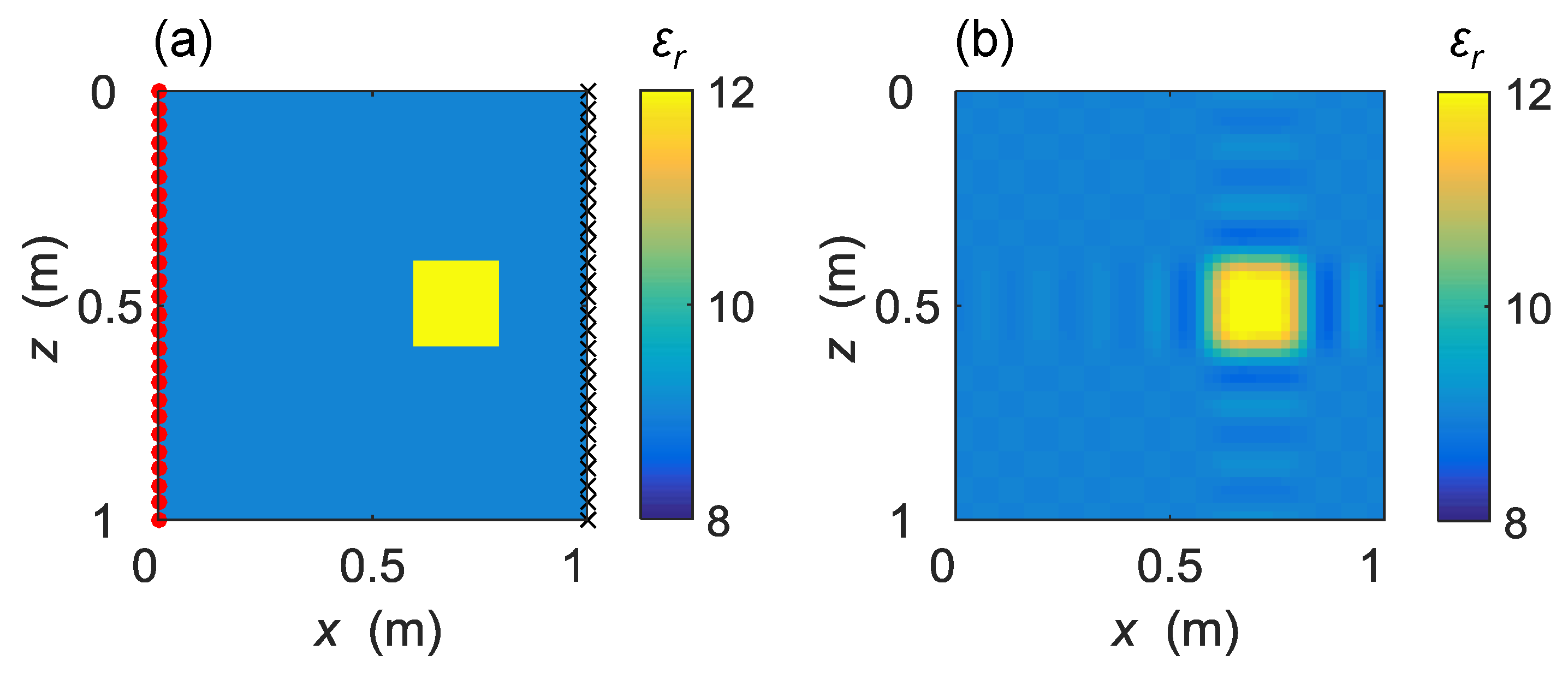
We now use a synthetic example to evaluate the performance of the straight-ray forward model compared with its FDTD counterpart. As illustrated in
Figure 1a, we create a 1.0 m × 1.0 m
field as the reference model, in which a 0.2 m × 0.2 m square-shaped target is simulated using
, higher than
for the surrounding medium. To simulate crosshole GPR measurements, the transmitting and receiving antennas are placed on the left and right side of the model, marked with red dots and black crosses, respectively. Multi-offset gathering (MOG) is used to collect data with step length of 0.02 m for both transmitting and receiving antennas. For each position of the transmitting antenna, GPR data are recorded at all receiving antenna locations. This results in 51 × 51 transmitting-receiving antenna pairs and a total number of 2601 crosshole GPR data.
We first discretize the reference model (
Figure 1a) with grid size of 0.005 m × 0.005 m (fine-grid model) and implement the 2D-FDTD solver (gprMax-2D developed by Giannopoulos [
32]) to simulate the crosshole GPR experiment and extract first-arrival traveltimes for the 51 × 51 transmitting-receiving antenna pairs. Other setups of the FDTD modeling include Ricker source wavelet with central frequency of 500 MHz, time window of 20 ns, and perfectly matched layer (PML) boundary condition on each side of the model. We take the first-arrival traveltimes calculated by the fine-grid FDTD modeling as real data (plotted with red lines in
Figure 2, assuming that no modeling error is accounted for in this simulation.
We next investigate the modeling errors of the FDTD and straight-ray models with grid size of 0.02 m × 0.02 m (coarse-grid model), which is practical and computational affordable in Bayesian inversion. The same settings except for grid size are used for the FDTD calculations, and the simulated first-arrival traveltimes are depicted with black lines in
Figure 2. Meanwhile, we use the straight-ray forward model to generate first-arrival traveltimes, and show the data in
Figure 2 with blue lines. It is obvious that the crosshole GPR data simulated by the FDTD modeling (black lines) are much closer to the real data (red lines) than those (blue lines) calculated by the straight-ray modeling. Thus the straight-ray model suffers from bigger modeling errors compared with the FDTD counterpart.
We also consider the modeling errors caused by the DCT parameterization approach. In order to do so, we create a DCT representation (
Figure 1b) of the coarse-grid model (2500 grid cells) using 256 (16 × 16) lower order DCT-coefficients. Here we use the peak signal-to-noise ratio (PSNR) to quantify the quality of parameter reduction, which is a common used tool in image compression [
47]. PSNR is defined as
where
and
are the
matrix and its DCT realization, respectively. A larger PSNR value stands for the smaller distortion of image reconstruction. For the above case, we use 256 DCT-coefficients to recover the matrix with 2500 grid cells and derive the PSNR value of 35.12, well above the common threshold in image compression, meaning that the reconstructed model preserves the structural details with high fidelity [
41].
The green and pink dotted lines in
Figure 2 show the first-arrival traveltimes calculated with the DCT reconstructed model using the FDTD and straight-ray solvers, respectively. The lines almost overlap with the data simulated using the full-parameter model, providing us with confidence that the DCT approach can reduce the parameter dimensionality considerably without causing noteworthy modeling errors.
We now summarize the performances of FDTD and straight-ray forward models in
Table 1. As a benchmark, the error-free first-arrival traveltimes are created using the FDTD modeling with fine-grid (0.005 m × 0.005 m) parameterization. With the coarse-grid (0.02 m × 0.02 m) parameterization, the data simulated by the straight-ray modeling show a more than 7 times larger root mean squared-error (RMSE) than that simulated by the FDTD modeling, indicating that the straight-ray model may cause considerable modeling errors that bias the inversion result. With forward simulations using the DCT reconstructed model, neglectable difference can be observed between the reconstructed and full-parameter model, or, to be precise, the difference is less than 1% for both FDTD and straight-ray models. This is an encouraging result that the use of DCT for dimensionality reduction causes no further modeling errors. We also resort our attention to the computational requirements of the two forward models. For a single forward simulation of the 51 × 51 first-arrival traveltimes, the FDTD modeling takes about 9.5790 s while the straight-ray modeling uses only 0.0214 seconds, which is roughly 450 times faster for one run (The computing time is tested on a computer with an i7-7700 CPU and 16 GB RAM). Therefore, the straight-ray forward model is computationally efficient thus can help relieve CPU burden of the inversion work, whereas the side effect that it brings relatively high modeling errors to data should be considered and treated carefully, and this will be addressed in the next section.
4. Inversion Results
In this section we investigate the use of the straight-ray forward model in our Bayesian inversion framework. We first present the inversion results using the FDTD forward modeling with waveform data, followed by a detailed analysis of the impact of the modeling error and model structure constraint of the the straight-ray model on the inversion results, and conclude with a summary of the model performances.
We take the synthetic relative permittivity model of
Figure 1a as the reference model. Measurement data (GPR waveforms and first-arrival traveltimes) are created by the fine-grid (0.005 m × 0.005 m) FDTD modeling of 51 × 51 transmitting-receiving antenna pairs, and a total number of 2601 crosshole GPR observations are obtained. The simulated data are contaminated with artificial white noise with standard deviations of 3% of the simulated data, which are 2.06 (in amplitude) for waveform data and 0.24 ns for first-arrival traveltime data. These data serve as our measurement data set, and are used to infer the relative permittivity values in the following inversion cases.
MCMC simulation with the
algorithm is employed to explore the posterior distributions of model parameters (relative permittivity values). We use a Jeffreys prior (uniform distribution in the log-transformed space) [
48] for the relative permittivity values with the lower and upper bound of 6 and 15, respectively, and implement the likelihood function in the form of Equation (
6). To maximize the computational efficiency, we run the
algorithm in parallel by evaluating 4 Markov chains on different CPU-cores. We also set the number of crossover values to 20, and scaling factor of the jump rate 75% lower to raise the acceptance rate of proposals, while keep all other settings the default values of the algorithm.
4.1. FDTD Model with Waveform Data
The first inversion starts with the FDTD forward model and waveform data. A coarse-grid of 0.02 m × 0.02 m is used to discrete the model, resulting in a total of
relative permittivity values that need to be estimated. The DCT approach is used for dimensionality reduction and different number of DCT-coefficients are tested.
Figure 3 illustrates the inversion results using 64, 144 and 256 DCT-coefficients. For each case, the reconstructed posterior mean (left column) and maximum a-posterior (MAP) estimations (middle column) of the relative permittivity fields appear visually identical and both pinpoint correctly the higher
area (target). With more DCT-coefficients, the inversion resolution increases as the square-shape and sharp-boundary of the target become more clear. Also, the RMSE values of the posterior models (right column) decrease as the number of the DCT-coefficients increases, which means the larger number of the DCT-coefficients used the better the posterior models fit the data. However, due to the modeling error caused by the coarse-grid FDTD, the posterior RMSE values are greater than the measurement error (2.06 in amplitude) for all three cases.
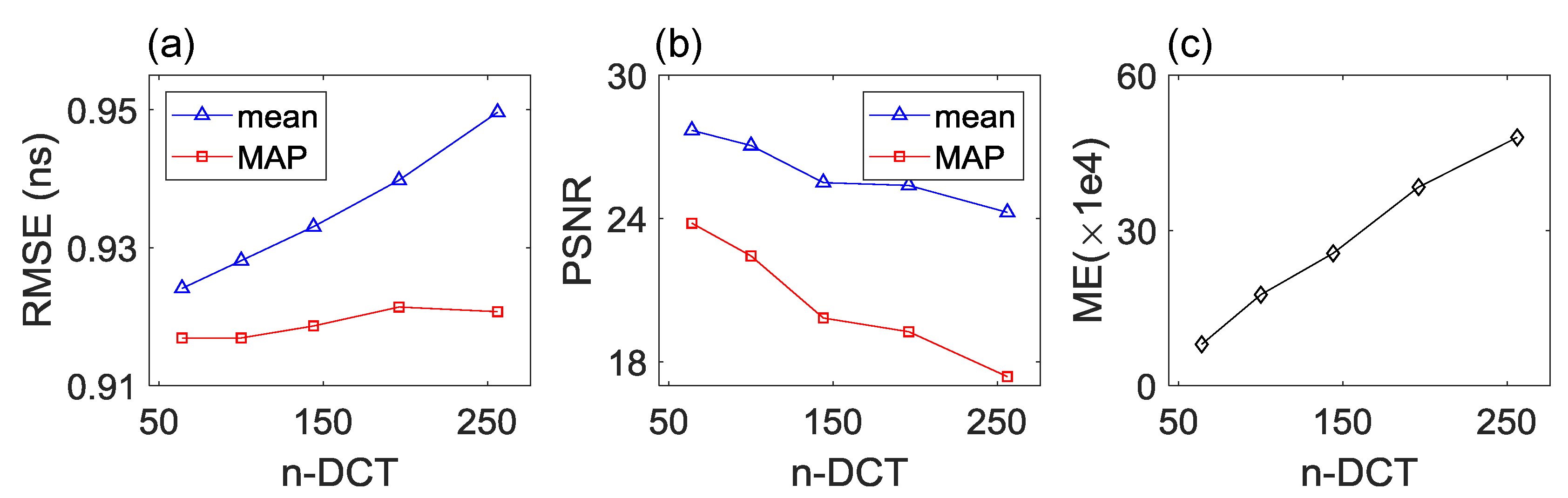
Figure 4 quantifies the impact of the number of DCT-coefficients on the inversion results. By investing more DCT-coefficients, the RMSE values (
Figure 4a) calculated using the posterior mean (blue lines with triangle markers) and MAP (red lines with square markers) models decrease from 3.65 to 2.54 that are in good agreement with the plots in
Figure 3c,f,i, indicating the improvement of data fit. The PSNR values (
Figure 4b) of the posterior mean and MAP models increase from 27.1 to 29.8 with the number of DCT-coefficients growing from 64 to 256, confirming the perspective stated in the visual inspection that better reconstructed
fields are obtained with more DCT-coefficients. Besides, all these PSNR values that are greater than 27 demonstrate that high fidelity of the reconstructed
fields is achieved using the FDTD forward model and waveform data. We also monitor the required number of model evaluations (ME) in
Figure 4c for the
algorithm to declare convergence and a total of 26,000, 68,000 and 136,000 model evaluations are needed for the three cases. An approximately linearly relation can be observed between the computational requirements and the number of DCT-coefficients.
4.2. Straight-Ray Model without Modeling Error Corrected
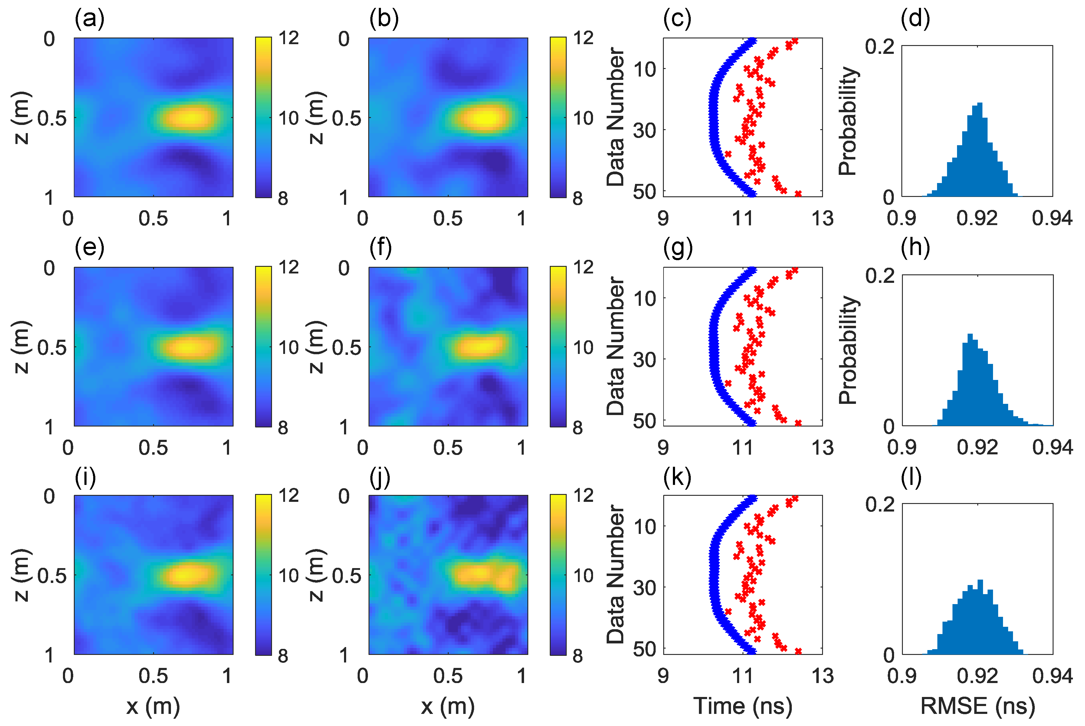
We now evaluate the use of the uncorrected straight-ray model in Bayesian inversion of crosshole GPR first-arrival traveltime data with the same settings of model discretization and dimensionality reduction as those of the FDTD model. The inversion results of using 64, 144 and 256 DCT-coefficients are considered and displayed in the top (a–d), middle (e–h) and bottom (i–l) rows in
Figure 5. It can be seen from the posterior mean and MAP realizations (the first and second columns) that the use of more DCT-coefficients deteriorates the inversion results. For the latter two cases using 144 and 256 DCT-coefficients, the posterior realizations exhibit significant variations that the target can no longer be resolved correctly. We plot in the third column the simulated first-arrival traveltimes of posterior models and the measurement data, and find the posterior models of the three cases fit the measurement data equally well. Note that although the RMSE values of the posterior solutions (the right column) are distributed very close to the measurement error (0.24 ns), the correct model parameters are not found. That is, without modeling error accounted for, there exists a set of incorrect parameters that can better match the measurement data than the true parameters do.
For a closer investigation of the inversion results, we see in
Figure 6a,b that the RMSE values are well around the measurement error, whereas the PSNR values are much smaller than those of the FDTD model. These PSNR values are under the common threshold that the reconstructed
fields hardly resemble the reference model. With more DCT-coefficients, the RMSE values of the posterior mean and MAP models increase while the PSNR values decrease, which means the use of more DCT-coefficients cannot improve the inversion results. Also, the required number of model evaluations grows with the number of DCT-coefficients. Compared with the FDTD model, ten times more model evaluations are needed when using the uncorrected straight-ray model. Therefore, the modeling error caused by the straight-ray model is remarkable and biases the inversion results considerably. Without modeling error corrected, even if the measurement data can be fit nicely, the inverted
fields differ greatly from the true model.
4.3. Straight-Ray Model with Modeling Error Corrected
To take into consideration the modeling error of the straight-ray simulator, we adopt the idea in [
38] that we first calculate an orthonormal basis for the modeling error using the fine-grid FDTD and coarse-grid straight-ray solvers prior to the inversion work. Then in MCMC, we use this basis to calculate the modeling error and subtract it from the residual the between simulated and measurement data before calculating the likelihood function.In this way the modeling error is isolated outside the Bayesian inversion and no longer biases the inversion results.
Figure 7 plots the inversion results using the straight-ray forward model with modeling error corrected. From the posterior mean and MAP realizations (the first and second columns) we can see improvements compared with the previous cases using the uncorrected forward model that the target can be identified in all three cases with 64, 144 and 256 DCT-coefficients. But like the uncorrected model example, with more DCT-coefficients, the reconstructed posterior mean and MAP models suffer from larger spatial variation that worsens the inversion results. It can be also seen that after modeling error is corrected, the simulated data do not closely fit the observations (the third column) and the RMSE values of the posterior solutions are much larger than the measurement error. This is because the simulated data incorporate the measurement and modeling errors. With the modeling error accounted for, the residuals between the simulated and measurement data need not to be minimized.
Figure 8 reveals similar patterns to those found in the uncorrected model example. The RMSE values increase and the PSNR values decrease with the number of DCT-coefficients, indicating that the use of more DCT-coefficients deteriorates the inversion results. Yet as a whole, the PSNR values derived from corrected models (
Figure 8b) are much larger than those of uncorrected models (
Figure 6b), demonstrating that the modeling error correction improves the inversion results considerably. Besides, after modeling error correction, only less than one quarter of model evaluations are needed for the parameters to reach convergence (
Figure 8c), which improves the computational efficiency obviously.
We now turn our attention to the impact of the number of DCT-coefficients. In the FDTD model example, the use of more DCT-coefficients improves the inversion results, whereas in the straight-ray model examples (both corrected and uncorrected), to increase the number of DCT-coefficients makes the inversion results even worse. We know that the DCT approach reduces the model parameters to a few DCT-coefficients. The more DCT-coefficients we use the higher the inversion resolution we can achieve, meanwhile the more unknowns we need to infer from data. Consider the FDTD model and the corrected straight-ray model, assuming that they both have no modeling errors, then the difference between the two examples is the data they use. In this work the FDTD model works with waveform data, while the straight-ray model works with first-arrival traveltime data. Although the 51 × 51 antenna pairs generate the same amount of waveform traces and first-arrival traveltimes, the number of data used for the FDTD inversion is far more than that for the straight-ray inversion as each trace contains hundreds of data points. In this work each trace contains 212 samples and a total of 551,412 data points are used for the FDTD inversion, yet for the straight-ray inversion the number of measurement first-arrival traveltimes is only 2601. Therefore, with the same amount of crosshole GPR measurements, the waveform data are much more informative to estimate more DCT-coefficients for a better description of the model structure, whereas the first-arrival traveltimes are insufficient and only a limited number of DCT-coefficients can be estimated correctly.
The choice of the number of DCT-coefficients is a trade-off between spatial resolution and uncertainty in the inversion results. In previous work we have introduced a method to determine the number of DCT-coefficients by examining the similarity between the reference model and its reduced order DCT representations [
28]. If some structural features of the subsurface can be used as prior information, a set of realizations can be generated from the training image (TI) and the DCT-coefficients with the occurrence probabilities larger than the threshold are considered as unknown model parameters in the inversion [
49]. One should be also aware that when using the first-arrival traveltimes as measurement data, the amount of data is always insufficient to infer a large number of unknown model parameters, thus a relatively small number of DCT-coefficients should be used for inversion.
4.4. Model Constraint
As a limited number of the first-arrival traveltime data is incapable of providing enough knowledge about the relatively large number of DCT-coefficients, while to increase considerably the amount of data is practically very expensive, we here learn the experience of deterministic inversion that to use a regularization term to decrease the ill-posedness of the inversion problem. In the view of the probabilistic inversion, the regularization term serves as the prior information that refines the range of model parameters [
40]. In this work, we impose a smooth constraint on the model structure by including Equation (
4) in the prior distribution. The regularization weight,
scales how much weight is assigned to the regularization term, and here we simply use the optimal value (
) calculated by maximizing the regularization term given the true model parameter values. Note that
can also be estimated together with model parameters in Bayesian inversion.
The inversion results using the corrected straight-ray forward model and constrained model structure are shown in
Figure 9. For all three cases using 64, 144 and 256 DCT-coefficients, the higher permittivity area is clearly depicted in the posterior mean and MAP realizations, and they appear no significant difference between each other. With modeling error accounted for, the simulated first-arrival traveltimes no longer closely fit the measurement data and the RMSE values of the posterior solutions are much larger than the measurement error. Note that with model constraint, the variation of simulated data becomes more modest than that of the previous example (
Figure 7). This reflects a smooth variation of the model structure when the model constraint is applied in the inversion.
As depicted in
Figure 10, the RMSE and PSNR values almost remain unchanged with the number of DCT-coefficients. This is because the regularization term reduces the model structure complexity and stabilizes the solution of the inverse problem. It can be also seen in
Figure 10b that the PSNR values of the cases using different number of DCT-coefficients stay around 27.8, indicating relatively high quality of the reconstructed models. The model constraint also decreases the required number of model evaluations (
Figure 10c) for the parameters to reach convergence to 60% of those using an unconstrained model (
Figure 8c).
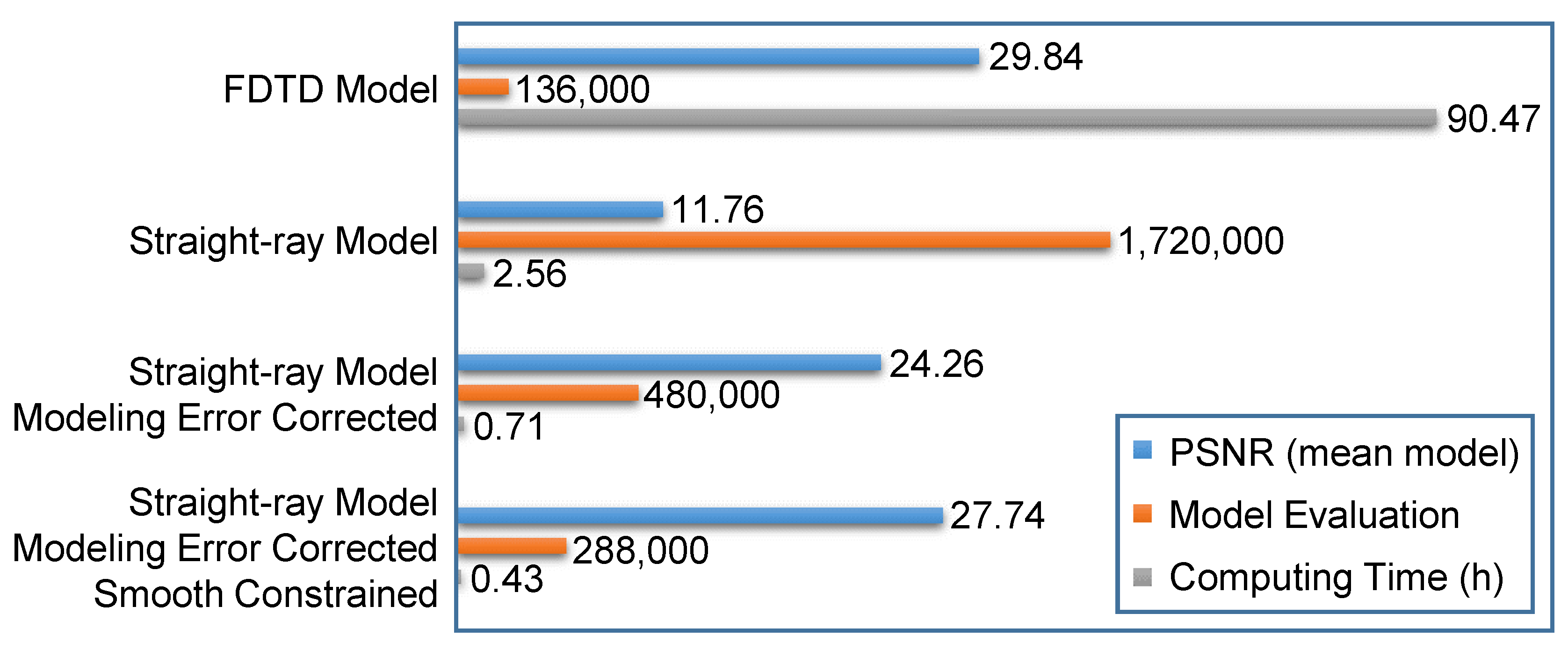
We conclude our numerical examples in
Figure 11 with a bar chart that summarizes the performance of different forward models in Bayesian inversion of crosshole GPR data. We use the PSNR values (blue bars) of posterior mean models to evaluate the inversion accuracy, and the number of model evaluations (orange bars) and computing time (gray bars) to measure the computational efficiency. The FDTD model with waveform data has the merit of the highest inversion accuracy and requires the least number of model evaluations among the examples, yet suffers from significantly long computing time (90.47 h in this study) due to huge CPU demand of the FDTD modeling. The straight-ray forward model, on the other hand, has the advantage of higher computational efficiency. Although the required number of model evaluations are much larger than that of the FDTD model, the inversion work takes far less computing time. However, due to modeling error, the straight-ray model cannot reconstruct the
field correctly and leads to a low PSNR value (11.76). By correcting the modeling error and constraining the model structure, the PSNR value is increased to 27.74 and the computing time is reduced to 0.43 h, which improves the inversion accuracy and computational efficiency considerably.
5. Conclusions
In Bayesian inversion of crosshole GPR data, the use of FDTD forward model with waveform data can generate posterior realizations with high accuracy, yet thousands to millions of model evaluations required by MCMC iterations are always computationally infeasible. We therefore in this paper turned our attention to a computational efficient straight-ray forward model and evaluated the applicability in the Bayesian inversion framework.
Based on a reference relative permittivity model, we calculated the first-arrival traveltime data using the FDTD and straight-ray solvers, respectively. With the same model grid size and measurement setup, the straight-ray simulator ran 450 times faster than the FDTD simulator, whereas suffered from more than 7 times larger modeling error. The DCT approach for dimensionality reduction was also tested in the forward simulations. We found that the dimensionality reduction using DCT contributed less than 1% to the modeling error.
We then performed Bayesian inversion of crosshole GPR first-arrival traveltime data with the straight-ray forward model using a set of synthetic examples. First the modeling error was disregarded and the straight-ray solver was used directly for forward calculations. In this case the measurement data were nicely fitted, yet the posterior realizations were not able to resemble the main features of the true model, and using more DCT-coefficients led to more unwanted artifacts in the posterior realizations. With modeling error accounted for, although the simulated first-arrival traveltimes no longer fit closely the measurement data, there were less unwanted features in the posterior realizations and the main features of the true model can be identified correctly. However, again, the inversion results became worse with an increased number of DCT-coefficients. Finally, we imposed a smooth constraint on the model structure and improved the inversion results considerably. No apparent unwanted features were observed in the posterior realizations and the number of DCT-coefficients had no significant impact on the inversion results. By investigating the computing time and PSNR values of the synthetic examples, we conclude that the use of the straight-ray forward model reduces the computational burden remarkably, meanwhile, with the modeling error corrected and model structure constrained, the inversion results are approximate to those of the FDTD model.
It should also be noted that the applicability of our inversion method is based on the evaluation of the synthetic example involving a moderate degree of nonlinearity. When the inverse problem is of a higher degree of nonlinearity, such as higher relative permittivity differences, larger object dimensions or in the presence of multiple objects, the straight-ray model we use, which is a linear model, might bias the inversion results. Future work will incorporate bending-ray based or artificial neural network (ANN) based forward kernels in our inversion framework to improve the capability of dealing with highly nonlinear inverse problems.


