Abstract
Impulsive noise is commonly present in many applications of actual communication networks, leading to algorithms based on the Gaussian model no longer being applicable. A robust parameter estimator of frequency-hopping (FH) signals suitable for various impulsive noise environments, referred to as ℓp-STFT, is proposed. The ℓp-STFT estimator replaces the ℓ2-norm by using the generalized version ℓp-norm where 1 < p < 2 for the derivation of the short-time Fourier transform (STFT) as an objective function. It combines impulsive noise processing with any time-frequency analysis algorithm based on STFT. Considering the accuracy of parameter estimation, the double-window spectrogram difference (DWSD) algorithm is used to illustrate the suitability of ℓp-STFT. Computer simulations are mainly conducted in α-stable noise to compare the performance of ℓp-STFT with STFT and fractional low-order STFT (FLOSTFT), Cauchy noise, and Gaussian mixture noise as supplements of different background noises to better demonstrate the robustness and accuracy of ℓp-STFT.
1. Introduction
The outstanding advantages of strong anti-jamming, a low interception rate, and a high-frequency spectrum utilization rate [1,2,3] have led to the rapid development of frequency hopping communication technology in military radio, military wireless communication, and civil wireless local area networks. Under the condition of less prior information, the blind parameter estimation of captured frequency-hopping (FH) signals is the core problem of FH communication. Accurate estimation parameters are helpful to monitor and interfere with enemy communications [4] and then steal enemy signals precisely and effectively, which is a crucial part of communication countermeasures.
The popular parameter estimation methods for FH signals mostly utilize a Gaussian model as background noise. However, a large amount of impulsive noise often occurs in the practical intricate noise environment, such as low-frequency atmospheric noise, low-voltage power communication, seismic signals, and radar clutter [5,6,7], which are characterized by remarkable impulses [8] and heavier tails. Since they have no second-order or higher moments, the performance of the existing time-frequency analysis methods based on the Gaussian noise model is usually unacceptable or even invalid: for example, the commonly used short-time Fourier transform (STFT), which is easy to calculate for simple principles [9]; Wigner–Ville distribution (WVD), with high time-frequency resolution; and pseudo-Wigner–Ville distribution (PWVD), with fewer cross-terms. Even improved algorithms that have been proposed in recent years will exhibit undesirable performance degradation, such as the spectrogram method, double-window spectrogram difference (DWSD) [10] method, and STFT-WVD joint algorithm.
For the processing of impulsive noise, reference [11] summarizes the sources of noise in the communication environment and demonstrates the correctness of modeling under α-stable distribution noise. A parameter estimation method based on fractional low-order (FLO) spectrum is proposed in reference [12], which can achieve accurate parameter estimation even at a low signal-to-noise ratio (SNR), but it is commonly directed to obtain linear frequency modulation signals. A parameter estimation algorithm is suggested in reference [13] based on second-order cyclic spectrum, which analyzes the relationship between the frequency and the corresponding second-order cyclic spectrum parameters. The estimation performance is good under high SNR, but poor in the case of low SNR. The median filtering method [14,15] has low computational complexity, but it blurs the characteristics of the signal while filtering out noise. Since the time-frequency distribution of the FH signal satisfies the sparse characteristic, some parameters estimation methods [16,17] are also proposed which are based on sparse time-frequency representation (STFD) of the signal obtained by establishing an optimization problem model. The signal parameter estimation technique under impulsive noise satisfies the requirements of security and interference in the complex communication environment, whereas many methods are not suitable for blind estimation of the parameters of FH signals.
Based on the above issues, we first focus on the impulsive noise processing problem by considering noise as the error [18] in the estimation. In many practical applications, squared error functions are insufficient in minimizing the magnitude of the estimation error. Therefore, under the premise that the least squares (LS) method makes less sense in impulsive noise, a more generalized method, the ℓp-norm [19], which has high tolerance to noise, will be a better choice to capture noise outliers. The ℓp-norm utilizes the minimum dispersion (MD) criterion instead of the minimum mean squared error (MMSE) criterion [20] to minimize the error between the estimated value and the true value. In other words, the ℓp-norm means minimizing the pth power of the error so that the fitted object can be infinitely close to the target.
Inspired by the fact that STFT is the mathematical basis of commonly used time-frequency analysis algorithms, it can be considered as the objective function of ℓp-norm estimation. Since STFT describes the energy change of the signal from two dimensions, time and frequency, the ensuing problem is that the objective function will change from a one-dimensional (1D) vector to a two-dimensional (2D) matrix. To resolve this problem, the matrix ℓp-norm estimation can be converted into a column vector ℓp-norm estimation. Then STFT will be used as a bridge to combine the ℓp-norm algorithm with the time-frequency analysis algorithm to accomplish parameter estimation of the FH signal while processing impulsive noise. An attractive and reliable method of accurate parameter estimation named ℓp-STFT is proposed in this paper.
The rest of the paper is organized as follows: In Section 2, we briefly review the impulsive noise distribution. The ℓp-STFT method is presented in detail in Section 3, where the steps of parameter estimation of FH signals are introduced. In Section 4, the computer simulation analysis demonstrates that the ℓp-STFT algorithm is superior to the STFT and fractional low-order STFT (FLOSTFT) algorithms in terms of accuracy and robustness. Some conclusions are drawn in Section 5.
2. Impulsive Noise Distribution
The α-stable distribution and Gaussian mixture distribution (GMD) are two basic and widely used empirical models for non-Gaussian noise.
If a random variable satisfies the α-stable distribution, its characteristic function has the following form:
where
with .
The α-stable distribution is completely determined by four unique parameters: α, β, γ, μ. The characteristic exponent α reflects the degree of the impulsive characteristics, which is embodied as the smaller the value of α, the stronger the impulse characteristics. The symmetry β determines the symmetry of the distribution. The dispersion γ is used to measure the extent to which the sample deviates from the mean, and finally, μ is the location parameter. If β = 0, γ = 1, and μ = 0, the distribution corresponds to the standard symmetric α-stable distribution (SαS). For α = 1 with β = 0 or α = 2, they correspond to two special cases of Cauchy distribution and Gaussian distribution [21], which is consistent with the implication of α.
The second-order GMD can be expressed as a weighted summation of two independent and identically distributed (IID) Gaussian distributions [22]; that is:
where is the weighting coefficient, which is used to control the ratio of impulsive noise to Gaussian noise; and , and , are the mean and variance of the Gaussian distribution, and the impulse characteristics are represented by the large difference between the two variances; that is, . Figure 1 shows the magnitude of the Cauchy noise, the standard SαS noise, and mixed Gaussian noise in the time domain.

Figure 1.
Time-domain waveform diagrams of impulsive noise under different conditions: (a) Cauchy noise with α = 1; (b) standard symmetric α-stable (SαS) noise with α = 1.2; (c) mixed Gaussian noise.
3. Proposed Algorithm
The received FH signal is formulated as:
with ; A is a numerical constant denoting the amplitude of the FH signal; denotes a rectangular window; and are the hopping period and hopping frequency to be estimated separately; and represents the impulsive noise.
3.1. Implementation of ℓp-STFT
The definition of STFT indicates that a long non-stationary signal is transformed into a short stationary signal matrix by adding a window function in the signal time domain, then perform DFT (Discrete Fourier Transform) on the windowed signal matrix to obtain the time-frequency spectrum matrix. Therefore, the 1D signal model is innovatively represented as a 2D signal matrix:
where denotes a reconstructed data matrix and has the form
denotes the time-frequency spectrum matrix that needs to be estimated. The coefficient matrix is a complex component matrix, where denotes a steering vector with , . is the short discrete stationary signal that is achieved by moving the position of the window function on the observed signal at a different time. Since the window function length is less than the estimated spectrum length , that is , the zero-padding on signal matrix is required. is the impulsive noise. The estimation task is to construct the above STFT cost function to obtain time-frequency spectrum from signal mixed with impulsive noise.
In conventional estimators, the cost function of spectrum estimation by DFT is in form of ℓ2-norm, which is exploited in reference [18]. Considering the relationship between STFT and DFT, we know that the cost function of STFT has the same form of ℓ2-norm, that means the estimation of , denoted by , can be obtained by
which corresponds to ℓ2-norm minimization, and represents the ℓ2-norm. Note that is corresponding to the spectrum obtained by directly performing STFT on the FH signal. To illustrate this point visually, we verify this result in the first part of simulation.
It is well known that the LS solution is equivalent to the maximum likelihood (ML) estimate when noise is a zero-mean white Gaussian process. In fact, it was also verified in reference [23] for LS-based parameter estimation in the presence of white Gaussian noise via several representative signal processing examples. Nevertheless, the validity of the Gaussian assumption is approximate at best, while the occurrence of non-Gaussian noise is common in many fields. In particular, if the noise is impulsive noise, unreliable parameter estimation will result, since the performance of the ℓ2-norm minimizer is very sensitive to outliers. To achieve robust estimation, ℓp-norm minimization with 1 < p < 2 is widely used since it is less sensitive to outliers than the square function. In this work, we focus on the cost function of ℓp-norm .
where the matrix ℓp-norm commonly uses an easier form defined as
In light of the ℓp-STFT model, it first calculates the initial spectrum of without filtering the outliers. Then, the powerful iterative reweighted least squares (IRLS) algorithm [24] is employed to eliminate the noise interference. One thing to point out is that the cost function of ℓp-STFT is a matrix that needs to be converted to column vectors before processing noise by IRLS [25]. IRLS will continuously iterate the weight matrix to obtain a satisfactory solution that converges to optimal accuracy. Finally, a time-frequency analysis algorithm via ℓp-STFT is constructed.
Since each column in matrix is independent, we can convert a big equation of the cost function matrix into small questions of N vectors [26] to tackle. That is, the matrix objective function of Equation (9) can be further expressed as
where and are the nth column of and , respectively. From there we can separately process the ℓp-norm of each column vector and then arrange the processed N sub-problems into a matrix in order, which is the time-frequency spectrum we ultimately need. Now the vector data model can be written as:
where and . Equation (11) is solved by minimizing the vector objective function as follows:
with . Employing (12) yields:
To solve Equation (13), IRLS is applicable to settle such minimizing cost function problem of ℓp-norm. It starts with a rough estimate of vector and then adjusts the weight coefficient to gradually approximate the optimal value. The objective function can be reformulated as
It is not difficult to obtain the matrix form of Equation (14), and it can be expressed as
where
is a diagonal weighting matrix represented by a residual vector; that is, . We further analyze Equation (16) to get the estimate of as
However, here is taken as a function of , and is also taken as a residual function of , and we cannot get the optimal estimate of in one step. Usually, all elements in the weighted matrix are initially set to , and the initial value of vector can be given by
The core of the IRLS method lies in continuously updating the estimated vector by updating weighted coefficients that utilize the previous residual vector. After each iteration of vector , IRLS will automatically judge whether it converges. If the accuracy requirement does not meet the tolerance ε, which is an extremely small positive number, it will continue iterating to guarantee convergence.
Afterwards, following the order of the previous matrix vectorization, we rearrange the series of vectors processed by ℓp-STFT into a time-frequency matrix in order:
At this point, we choose an appropriate time-frequency analysis algorithm and construct it via the previously generated ℓp-STFT. The complete ℓp-STFT algorithm is summarized in Algorithm 1.
| Algorithm 1: For ℓp-norm short-time Fourier transform (ℓp-STFT) |
| 1. Reconstruct the original signal into a signal matrix and build the STFT cost function. |
| 2. Simplify the matrix ℓp-norm optimization into sequential vector ℓp-norm optimization. |
| 3. Initialize the weighted matrix with and the estimated with . |
| 4. Compute the residual vector and use to reconstruct the weighting matrix . |
| 5. Update . |
| 6. Repeat steps 4 and 5 until to get the updated . If , stop the iteration; otherwise, go to step 4. |
| 7. Arrange the vectors into a time-frequency matrix in order. |
| 8. Construct time-frequency analysis algorithm using a ℓp-STFT spectrum matrix. |
3.2. Parameter Estimation Based on ℓp-STFT
As usual, whether it is directly acquiring the characteristics of the FH signal for tracking interference or further constructing the local oscillator signal to steal enemy information, the blind estimation of parameters is a necessary condition for the next step. The double-window spectrogram difference (DWSD) method has a superior time-frequency representation that can accurately estimate important parameters such as hopping period, hopping frequency, hopping time set, and hopping rate. More specifically, the spectrogram (SPEC) method should be performed using a long window function and short window function , respectively on signal to obtain the time-frequency transform results. Combining the two sets of results with better time and frequency resolution will provide the time-frequency analysis of DWSD. The definition of DWSD is given as
where
using the ℓp-STFT method to eliminate the presence of outliers and acquire the and . The normalized Stankovic entropy measure is an effective criterion used for evaluating the time-frequency concentration in the spectrogram [10], which has the expression
where denotes the signal entry of time-frequency distribution that is affected by the length of the window function. The smaller the value of , the better the time-frequency performance and the more optimal the length of the window function.
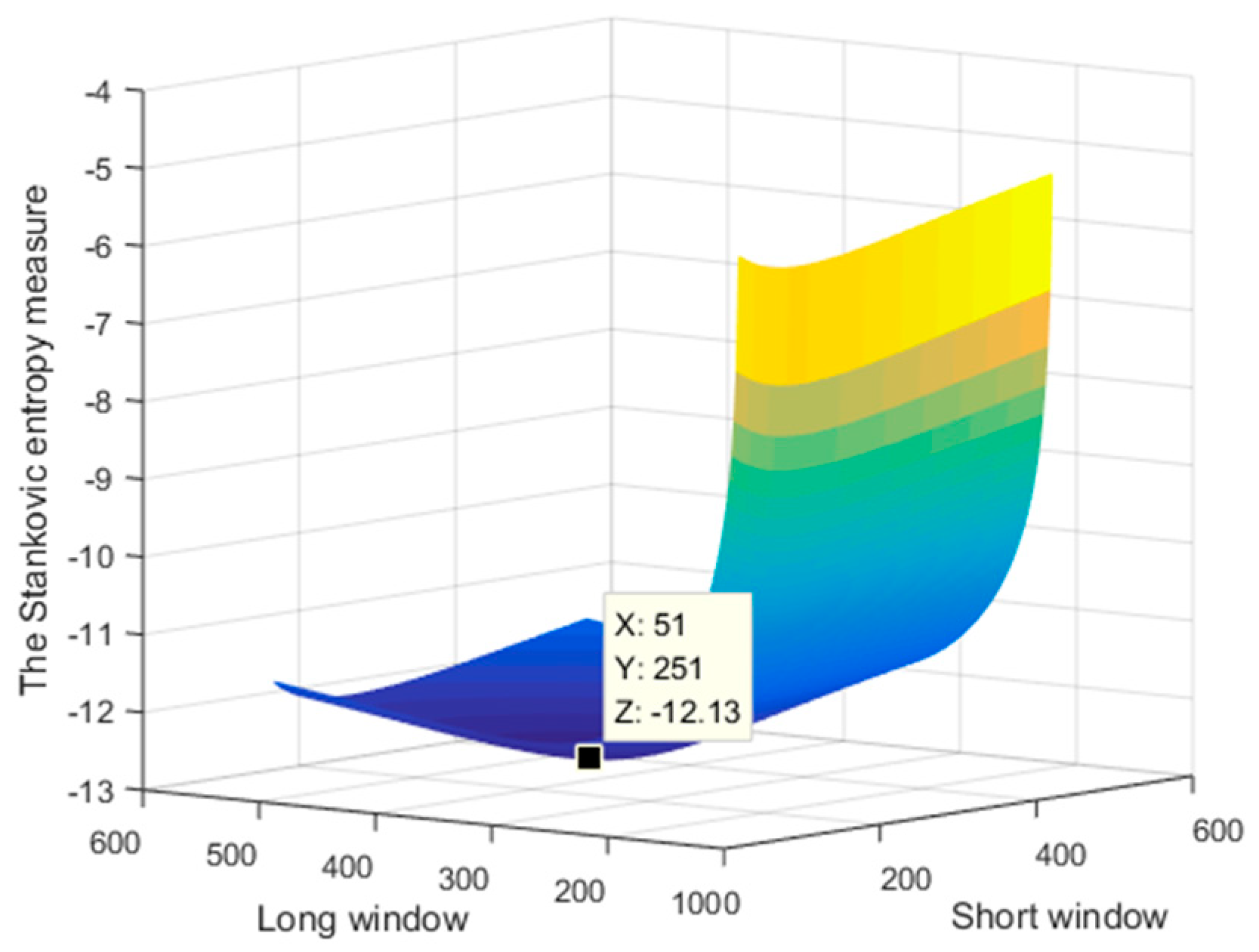
Suppose N equals the length of signal, Figure 2 shows the curve of entropy measure obtained by simultaneously varying the length of long window and the short window between 0~N/2 and N/8~5N/8 in a same sampling step. When the short window ranges from N/20 to 9N/40 and the long window ranges from N/4 to 9N/20, we can obtain a better time-frequency performance.

Figure 2.
The Stankovic entropy measure versus length of window function.
Afterwards, we can apply the treated ℓp-STFT spectrum to construct the crucial time-frequency diagram even in an impulsive noise environment. The can be expressed as
To more conveniently and clearly estimate parameters, we can take the maximum value of the time-frequency diagram to obtain the time-frequency ridge line, as shown in Figure 5b.
Performing first-order difference on the time-frequency ridge line will produce a frequency difference sequence .
The time domain position of the value in is an equally spaced difference sequence , which corresponds to the hopping time set. The estimated hopping period is the mean value of a set of the hopping period approximations, which are acquired by performing first-order difference on .
Then we can easily estimate the hopping rate, which is the reciprocal of the hopping period and the hopping time set, because of the changeless hopping period.
The estimation of hopping frequency is also based on the time-frequency ridge line, and can be acquired by averaging the instantaneous frequency in each hopping period.
After obtaining the above parameters, it is not difficult to determine that the hopping period and hopping frequency are two basic parameters. The estimation accuracy of these two parameters is an important criterion to evaluate the performance of the ℓp-STFT algorithm.
4. Simulation Result and Analysis
Computer simulations were conducted to investigate the performance of the derived estimator. The signal is generated by Equation (4), where the parameters in the FH signal are set as follows: eight hopping periods with , the sampling rate = 10 kHz, the sampling point N = 800, the hopping frequencies = {0.5, 2.5, 1, 3.5, 2, 3, 1.5, 4} kHz, and the noise being standard SαS noise with α = 1.5, β = 0, γ = 1. Since impulsive noise has no finite second-order moment, the generalized signal-to-noise ratio (GSNR) [27] will be more applicable than the traditional signal-to-noise ratio, and is set to 3 dB. The order of ℓp-STFT satisfies 1 < p < 2, p = 1.2, the explanation for p is given in Appendix A, and the tolerance is taken as ε = 1 × 10⁻⁴. All results were simulated using MATLAB running on Intel(R) Core(TM) i7-4790 CPU@3.60 GHz and Windows 10 for observations.
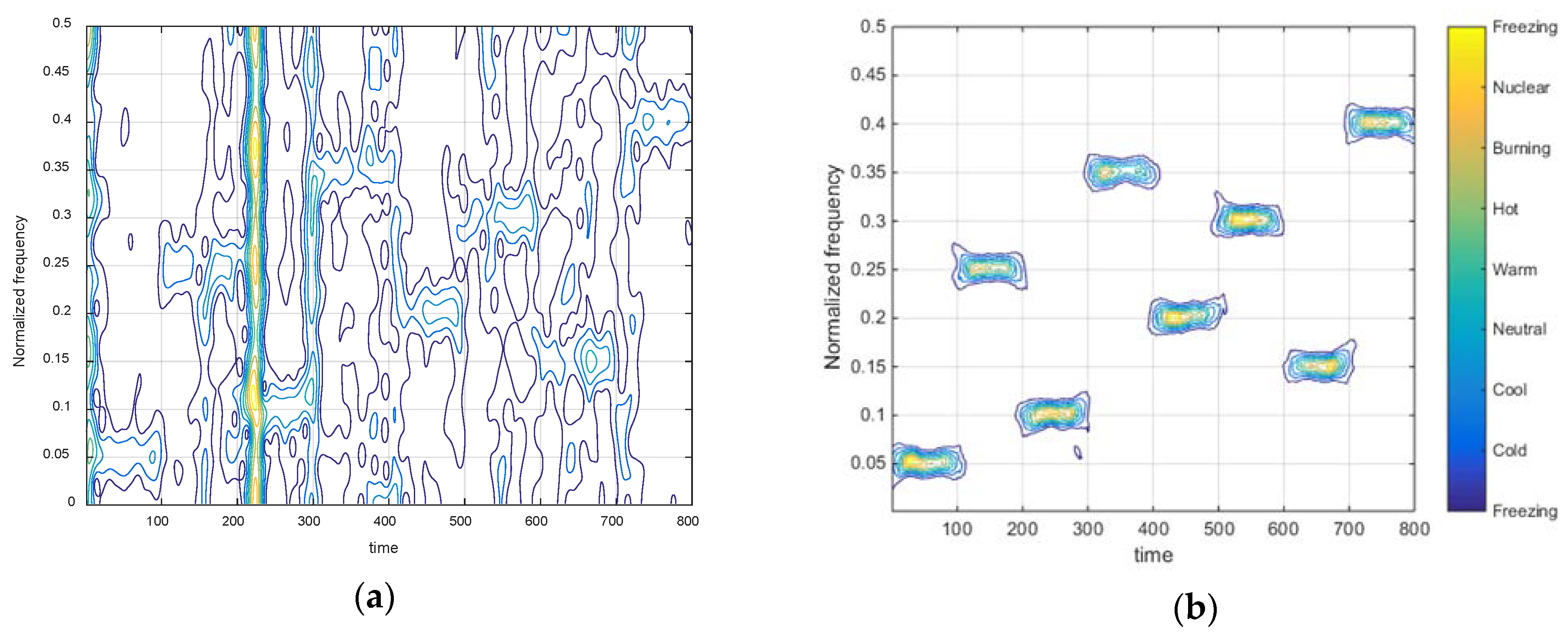
First, we verified the equivalence between the spectrogram obtained by STFT and the spectrogram estimated from the cost function of STFT based on ℓ2-norm. We select the length of the window function is 100 and carry out the experiment in non-noise environment to removal interference. Figure 3 shows that the time-frequency spectrograms produced by these two ways are almost consistent. It serves well to prove that the cost function of STFT is effective and the spectrogram obtained by STFT is equivalent to the spectrogram estimated by the cost function base on ℓ2-norm.
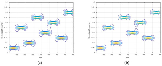
Figure 3.
Time-frequency spectrograms of short-time Fourier transform (STFT) obtained by (a) the STFT; (b) the cost function of STFT based on ℓ2-norm.
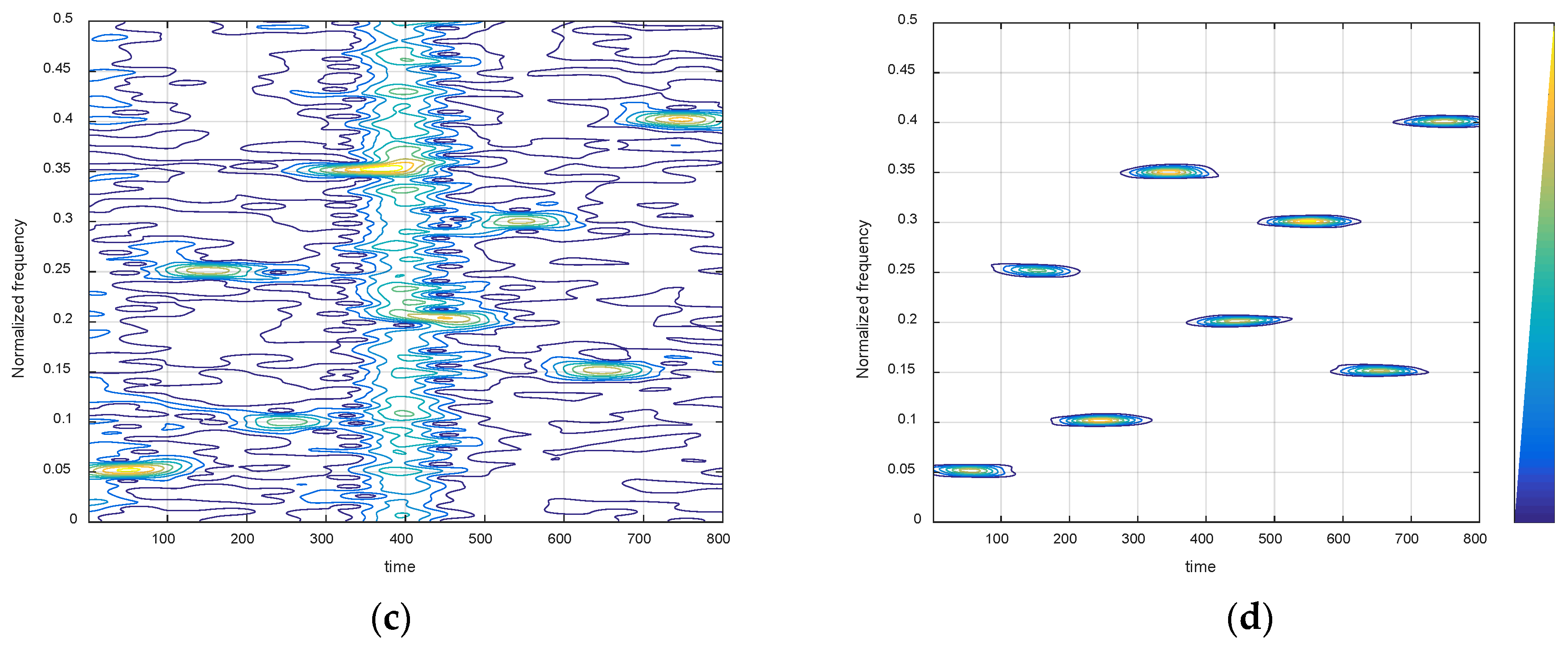
Second, we studied the performance of the proposed method applied to the DWSD algorithm in α-stable noise. The lengths of the long and short windows are 251 and 51, respectively. This means they are within the range we have illustrated and the selection of window function length is suitable for the DWSD method. The time-frequency diagram of STFT with a narrow window function is shown in Figure 4a, which is also the initial spectrogram of ℓp-STFT. We can see that there are several impulse interferences that are maintained for a short time but with a high amplitude, as well as many small noise points, both of which seriously disturb the signal estimation. In contrast, the spectrogram in Figure 4b, which was obtained by ℓp-STFT, effectively extracts the energy of signal submerged in impulsive noise while removing noise outliers. In the same way, the result comparison of time-frequency diagrams using a wide window function are presented in Figure 4c,d. The result is consistent with the effect of ℓp-STFT adding the narrow window function. Therefore, ℓp-STFT provides excellent robustness that appears to be hardly affected by the characteristics of noise outliers. Then, Figure 5a,b shows the time-frequency diagram and the time-frequency ridge line of ℓp-DWSD, which combines the above two sets of optimal results processed by ℓp-STFT. ℓp-DWSD exhibits extraordinarily powerful time-frequency concentration and accurately describes the parameter information of FH signals, even in an impulsive noise environment.
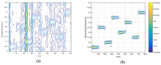
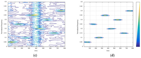
Figure 4.
Time-frequency spectrograms of STFT with different window functions in impulsive noise. (a) Initial spectrogram with narrow window function; (b) spectrogram of ℓp-STFT with narrow window function; (c) initial spectrogram with wide window function; (d) spectrogram of ℓp-STFT with wide window function.
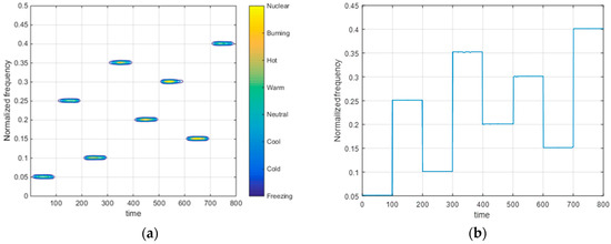
Figure 5.
(a) Time-frequency spectrogram and (b) time-frequency ridge line of ℓp-double-window spectrogram difference (DWSD).
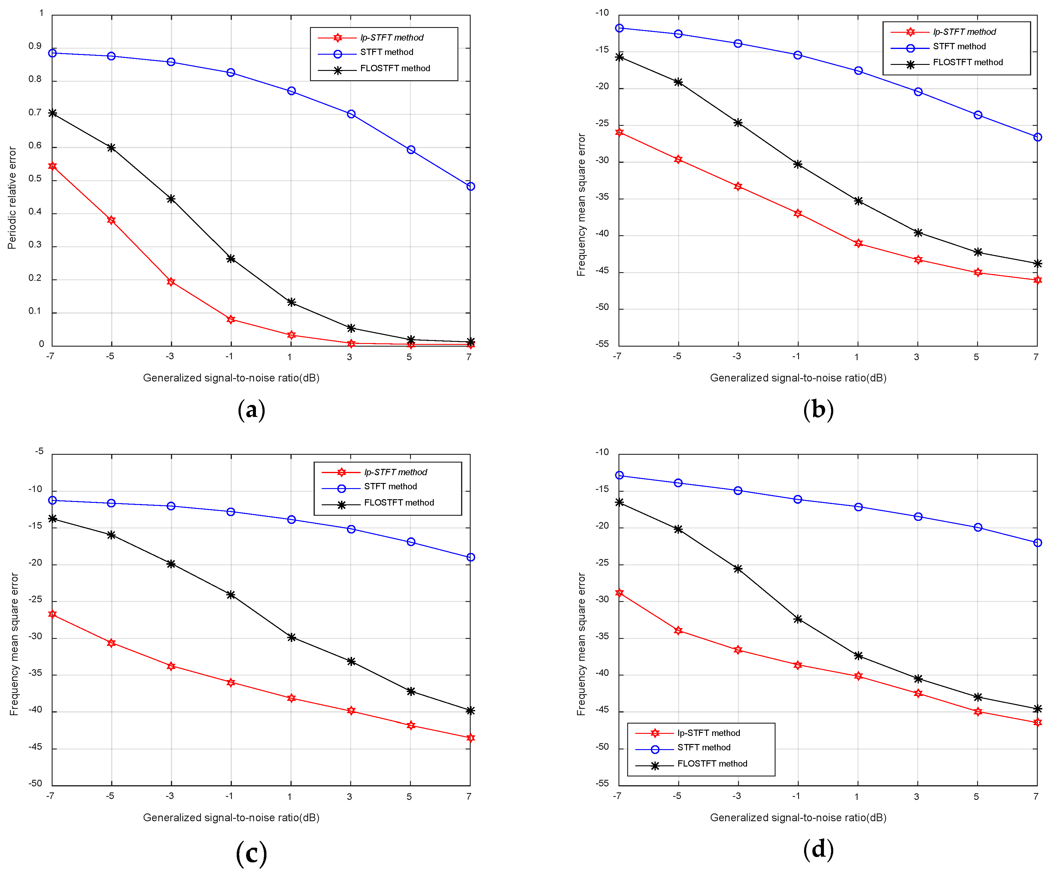
Third, we selected the algorithms related to the STFT to compare the performance of parameter estimation: STFT, FLOSTFT, and ℓp-STFT. The FLOSTFT method represents a class of algorithms based on fractional low-order statistics, and the fractional lower moments assumes p = 0.4. After repeating 100 experiments on these three methods in α-stable noise with α = 1.2, β = 0, γ = 1, we compared the relative error of hopping period and the mean squared error (MSE) of hopping frequency to evaluate their parameter estimation performance.
On the one hand, in terms of the estimated performance of the hopping period that is shown in Figure 6a, the accuracy of STFT without any processing is the worst among the three methods but is also the most primitive. STFT can be used as an intuitive indicator of performance comparison. From the holistic perspective of the curve, the larger the impulse amplitude, the lower the fault tolerance of the algorithm and the worse the performance becomes. When GSNR > 3 dB, both FLOSTFT and ℓp-STFT methods almost accurately estimate the hopping period and maintain stable estimation under high GSNR, and for STFT, the same result requires a higher GSNR to be completed, while the robustness of the algorithm under low GSNR can better prove the superiority of the algorithm. From Figure 4a we can find that, first, at low GSNR, the overall performance of the ℓp-STFT algorithm is superior to FLOSTFT and FLOSTFT is better than STFT. Second, the periodic relative error curve of the ℓp-STFT algorithm has the fastest rate of decline compared with the other two methods. Furthermore, at GSNR = 1 dB, the relative error value of ℓp-STFT is almost equal to zero. This effectively demonstrates that the ℓp-STFT algorithm not only maintains stable and accurate estimation at high GSNR, but also quickly achieves relatively high parameter estimation accuracy at low GSNR.
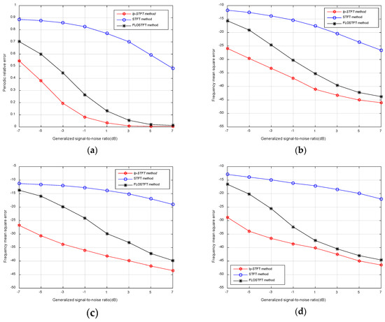
Figure 6.
Performance comparison of STFT, fractional low-order STFT (FLOSTFT), and ℓp-STFT methods versus generalized signal-to-noise ratio (GSNR). (a) Periodic relative error of hopping period; (b) mean squared error (MSE) of hopping frequency in α-stable noise; (c) MSE of hopping frequency in Cauchy noise; (d) MSE of hopping frequency in Gaussian mixture noise.
On the other hand, from the perspective of estimating the performance of the hopping frequency, in addition to α-stable noise, Cauchy noise with α = 1 and GWD noise with ε = 0.03, μ = 0, , are also used as impulsive noise environments to better illustrate the robustness of the ℓp-STFT algorithm. Comparing the MSE curve of the three methods presented in Figure 6b–d in any kind of noise environment, ℓp-STFT has higher accuracy for frequency estimation than the other two methods. For Figure 6b, with smaller impulsive amplitudes, when GSNR < 0 dB, the estimated performance of FLOSTFT is seriously degraded, whereas ℓp-STFT can still estimate the hopping frequency comparatively accurately, and this point is more evident in the Cauchy noise environment of Figure 6c. The strong impulsive noise features further highlight the advantages of ℓp-STFT, and the estimation precision of ℓp-STFT is nearly 10 dB higher than FLOSTFT when GSNR < 0 dB. Figure 6d showing GWD noise represents the case where the impulse appears more frequently, and the noise removal effect of the ℓp-STFT algorithm is still the best under this scenario, at about 8 dB higher than FLOSTFT in low GSNR. Even when GSNR > 0 dB, although the estimated performance of both algorithms is improved, ℓp-STFT is also maintained at nearly 3 dB higher than FLOSTFT for all impulsive noise environments. This result convincingly proves the robustness of ℓp-STFT to outliers and the accuracy of parameter estimation in the face of strong impulsive noise.
5. Conclusions
Almost all algorithms approximately applicable to the Gaussian distribution model have varying degrees of performance degradation in an impulsive noise environment. To solve such a knotty problem, a new algorithm called ℓp-STFT is proposed for robust and accurate parameter estimation of FH signals. It takes STFT as an associated bond to combine the ℓp-norm algorithm with the time-frequency analysis algorithm. The simulation results demonstrate that the ℓp-STFT method has strong robustness and parameter estimation accuracy, especially in low-GSNR environments. However, the computational complexity caused by iteration requires further research in the future.
Author Contributions
Conceptualization, Y.S., L.W., Y.C. and X.Y.; methodology, Y.S. and L.W.; software, Y.S. and L.W.; validation, Y.S., L.W. and Y.C.; formal analysis, Y.C. and X.Y.; writing—original draft preparation, Y.S., L.W., Y.C. and X.Y.; writing—review and editing, Y.S., L.W., Y.C. and X.Y.; visualization, Y.S. and L.W.; supervision, Y.C. and X.Y.; funding acquisition, L.W. and Y.C.
Funding
This research was funded by the National Natural Science Found of China under grant number 61701021 and 61701020.
Conflicts of Interest
The authors declare no conflict of interest.
Appendix A
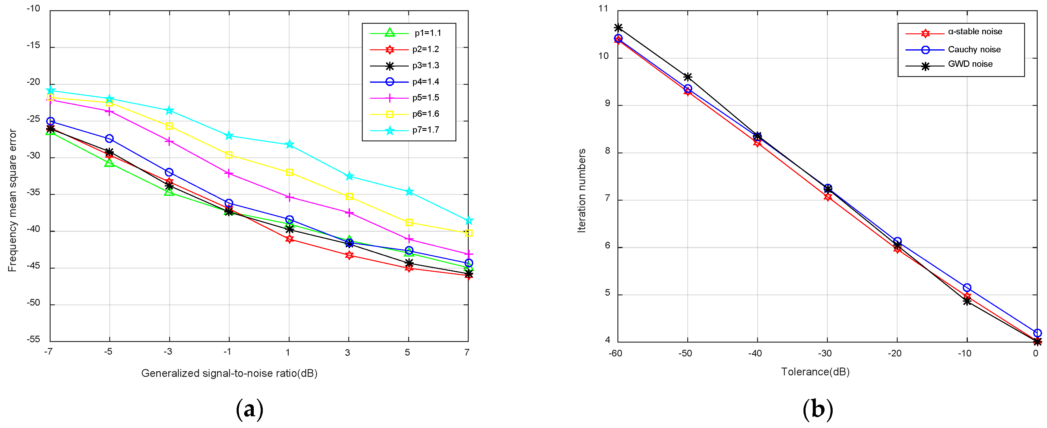
We explore the choice of order p, which is important in the proposed method. In 50 repeated experiments in α-stable noise, seven values of p from large to small were selected to compare the impact on ℓp-STFT. As shown by the MSE of hopping frequency in Figure A1a, it is not difficult to find that ℓp-STFT with a smaller order p has better estimation performance. It is difficult to find the optimal p precisely, whereas the performance of ℓp-STFT is generally consistent and satisfactory when the order p within the range 1.1 ≤ p ≤ 1.4. Hence the p we need is not necessarily the best but a suitable one, and p = 1.2 is preferred in ℓp-STFT.
Appendix B
The convergence rate of ℓp-STFT method in α-stable noise, Cauchy noise and GWD noise are also compared. In fact, we primarily care about the number of iterations of ℓp-STFT method under different tolerances. Seven tolerances are taken for verification, that are ε = 1 × 10⁻⁶, 1 × 10⁻⁵, 1 × 10⁻⁴, 1 × 10⁻³, 1 × 10⁻², 1 × 10⁻¹ and 1 × 10−0. From the Figure A1b we observed that the proposed algorithm has similar convergence rate under different impulsive noises, which has a linear approximation relationship to the tolerance accuracy. In addition, it can be seen that for the tolerance ε = 1 × 10⁻⁴ we provided, the relative error is less than the tolerance after 9 iterations.
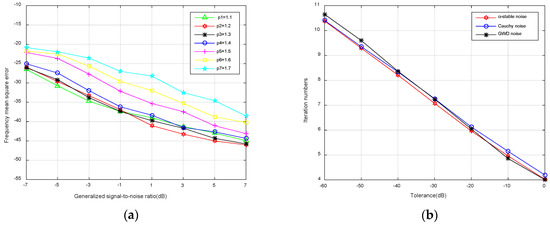
Figure A1.
(a) MSE of hopping frequency with p = 1.1, 1.2, 1.3, 1.4, 1.5, 1.6, 1.7; (b) Number of iterations versus tolerance.
Figure A1.
(a) MSE of hopping frequency with p = 1.1, 1.2, 1.3, 1.4, 1.5, 1.6, 1.7; (b) Number of iterations versus tolerance.
References
- Jin, Y.; Liu, J. Parameter estimation of frequency hopping signals in alpha stable noise environment. In Proceedings of the International Conference on Signal Processing, Beijing, China, 21–25 October 2012; pp. 250–253. [Google Scholar]
- Fan, H.N.; Guo, Y.; Meng, Q.W. Blind parameter estimation of frequency-hopping signals based on atomic decomposition. In Proceedings of the 2009 First International Workshop on Education Technology and Computer Science, Wuhan, China, 7–8 March 2009. [Google Scholar]
- Chen, T.C. Joint signal parameter estimation of frequency-hopping communications. IET Commun. 2012, 6, 381–389. [Google Scholar] [CrossRef]
- Liu, S.H.; Zhang, Y.M. Structure-aware Bayesian compressive sensing for frequency-hopping spectrum estimation with missing observations. IEEE Trans. Signal Process. 2018, 66, 2153–2166. [Google Scholar] [CrossRef]
- Jin, Y.; Liu, J. Parameter estimation of frequency hopping signals based on the robust S-transform algorithms in alpha stable noise environment. AEU-Int. J. Electron. Commun. 2016, 70, 611–616. [Google Scholar] [CrossRef]
- Yue, B.B.; Peng, Z.M.; He, Y.M. Impulsive noise suppression using fast Myriad filter in seismic signal processing. In Proceedings of the International Conference on Computational and Information Sciences, Shiyang, China, 21–23 June 2013. [Google Scholar]
- Amirshahi, P.; Navidpour, S.M.; Kavehrad, M. Performance analysis of uncoded and coded OFDM broadband transmission over low voltage power-line channels with impulsive noise. IEEE Trans. Power Deliv. 2006, 21, 1927–1934. [Google Scholar] [CrossRef]
- Yang, C.; Zhang, Y.; Jian, Y. Structure-adaptive fuzzy estimation for random-valued impulse noise suppression. IEEE Trans. Circuits Syst. Video Technol. 2016, 28, 414–427. [Google Scholar]
- Tong, L.; Tang, Y.; Lv, J. Parameter estimation of FH signals based on STFT and music algorithm. In Proceedings of the International Conference on Computer Application and System Modeling, Taiyuan, China, 22–24 October 2010. [Google Scholar]
- He, Y.; Su, Y.; Chen, Y. Double window spectrogram difference method: A blind estimation of frequency-hopping signal for battlefield communication environment. In Proceedings of the Asia-Pacific Conference on Communications, Ningbo, China, 12–14 November 2018; pp. 439–443. [Google Scholar]
- Tsihrintzis, G.A.; Nikias, C.L. Performance of optimum and suboptimum receivers in the presence of impulsive noise modeled as an alpha-stable process. IEEE Trans. Commun. 1995, 43, 904–914. [Google Scholar] [CrossRef]
- Gu, G.D.; Zhang, Y.S.; Tian, B. Estimation of LFM signal’s time parameters under the alpha-stable distribution noise. In Proceedings of the IEEE Circuits and Systems International Conference on Testing and Diagnosis, Chengdu, China, 28–29 April 2009. [Google Scholar]
- Zhao, C.H.; Yang, W.C.; Cheng, B.Z. Parameter estimation of MPSK signals in alpha stable distribution noise environment. J. Shenyang Univ. Technol. 2013, 35, 194–199. [Google Scholar]
- Wierzchowski, W.; Pawełczyk, M. Median filtering approach for active control of impulsive noise. In Proceedings of the International Conference on Methods and Models in Automation and Robotics, Miedzyzdroje, Poland, 2–5 September 2014. [Google Scholar]
- Ismaeil, M.; Pritamdas, K.; Devi, K.J.K. Performance analysis of new adaptive decision based median filter on FPGA for impulsive noise filtering. In Proceedings of the International Conference on Electronics, Materials Engineering and Nano-Technology, Kolkata, India, 28–29 April 2017. [Google Scholar]
- Kowalski, M. Sparse regression using mixed norms. Appl. Comput. Harmon. Anal. 2009, 27, 303–324. [Google Scholar] [CrossRef]
- Gardner, T.J.; Magnasco, M.O. Sparse time-frequency representations. Proc. Natl. Acad. Sci. USA 2006, 103, 6094–6099. [Google Scholar] [CrossRef] [PubMed]
- Ming, X.; Xu, L.; Jian, L. IAA spectral estimation: Fast implementation using the Gohberg–Semencul factorization. IEEE Trans. Signal Process. 2011, 59, 3251–3261. [Google Scholar] [CrossRef]
- Li, T.H. A nonlinear method for robust spectral analysis. IEEE Trans. Signal Process. 2010, 58, 2466–2474. [Google Scholar] [CrossRef]
- Chen, B.S.; Chen, J.M.; Shern, S.C. An ARMA robust system identification using a generalized ℓp-norm estimation algorithm. IEEE Trans. Signal Process. 1994, 42, 1063–1073. [Google Scholar] [CrossRef]
- Kuruoglu, E.E.; Fitzgerald, W.J.; Rayner, P.J.W. Nonlinear autoregressive modeling of non-Gaussian signals using l/sub p/-norm techniques. In Proceedings of the IEEE International Conference on Acoustics, Speech, and Signal Processing, Munich, Germany, 21–24 April 1997. [Google Scholar]
- Zhao, X.; Li, F. Sparse Bayesian compressed spectrum sensing under Gaussian mixture noise. IEEE Trans. Veh. Technol. 2018, 67, 6087–6097. [Google Scholar] [CrossRef]
- So, H.C.; Chan, Y.T.; Chen, Y. Simple formulas for bias and mean square error computation. IEEE Signal Process Mag. 2013, 30, 162–165. [Google Scholar]
- Lai, M.J.; Xu, Y.; Yin, W. Improved iteratively reweighted least squares for unconstrained smoothed ℓp minimization. Siam J. Numer. Anal. 2013, 51, 927–957. [Google Scholar] [CrossRef]
- Wen, F.; Liu, W. Iteratively reweighted optimum linear regression in the presence of generalized Gaussian noise. In Proceedings of the IEEE International Conference on Digital Signal Processing, Beijing, China, 16–18 October 2016. [Google Scholar]
- Zeng, W.J.; So, H.C.; Huang, L. ℓp-MUSIC: Robust direction-of-arrival estimator for impulsive noise environments. IEEE Trans. Signal Process. 2013, 61, 4296–4308. [Google Scholar] [CrossRef]
- Li, L.; Nicolas, H.; Shi, X.F. Joint Estimation of Doppler Stretch and Time Delay of Wideband Echoes for LFM Pulse Radar Based on Sigmoid-FRFT Transform under the Impulsive Noise Environment. Electronics 2019, 8, 121. [Google Scholar] [CrossRef]
© 2019 by the authors. Licensee MDPI, Basel, Switzerland. This article is an open access article distributed under the terms and conditions of the Creative Commons Attribution (CC BY) license (http://creativecommons.org/licenses/by/4.0/).


