Abstract
The analysis of seismic noise provides a reliable estimation of the soil properties, which supposes the starting point for the assessment of the seismic hazard. The horizontal-to-vertical spectral ratio technique calculates the resonant frequency of the soil just by using a single three-component sensor. Array measurements require at least several vertical sensors registering simultaneously and their analysis provides an estimation of the surface waves dispersion curve. Although these methods are relatively cheaper than other geotechnical techniques, the cost of the sensors and the multi-channel data acquisition system means that small research groups cannot afford this kind of equipment. In this work, two prototypes for registering seismic noise have been developed and implemented: a three-channel acquisition system, optimized for working with three-component sensors; and a twelve-channel acquisition system, prepared for working simultaneously with twelve vertical geophones. Both prototypes are characterized by being open-hardware, open-software, easy to implement, and low-cost. The main aim is to provide a data acquisition system that can be reproduced and applied by any research group. Both developed prototypes have been tested and compared with other commercial equipment, showing their suitability to register seismic noise and to estimate the soil characteristics.
1. Introduction
Ambient seismic noise corresponds to vibrations or fluctuations on the earth’s surface due to different natural and artificial causes. These vibrations are imperceptible to a human being, but not to seismic sensors. So, its record and analysis provides valuable information about the properties of the medium going through, and these are the characteristics of the soil. By means of different techniques, the estimation of the resonant frequency of the soil and the calculation of shear-wave velocity profiles provide valuable information to predict the soil response in case of an earthquake. Therefore, the analysis of ambient seismic noise for soil characterization (microzonation studies) constitutes the first step in the seismic hazard assessment of a region.
Therefore, in the last decades, ambient noise-based methods have become a suitable alternative to geotechnical prospections for investigating the subsoil properties. In contrast to other geotechnical and geophysical techniques, ambient noise methods are non-invasive and easier to implement, which makes them especially suited for urban areas. In fact, they only require the deployment of one or several sensors on the ground surface in order to measure the vibrations produced by different natural and human sources (the location of the sources is far enough from the recording area, so as to consider the register of plane wave fronts). The detected fluctuations present very small amplitude, around 10−10 to 10−2 m/s, and a bandwidth between 0.001 and 50 Hz [1]. Frequencies below 1Hz usually correspond to natural causes (atmospheric factors, tides, etc.), meanwhile frequencies above 1Hz usually correspond to human factors (traffic, industrial or urban activities, etc.) [2,3]. Both sources of noise are useful for the characterization of the subsoil. A complete review of the noise characteristics and its application to site effects studies can be found in the work of Bonnefoy-Claudet et al. [4].
The recording of the ambient seismic noise is carried out through the combination of one or several sensors and an acquisition system. The sensor acts as a transducer from velocity, displacement, or acceleration to electrical signal. For our application case, they are usually velocity sensors. Typical instruments used are short–period sensors, which present a high-pass behavior with cutoff frequency between 0.2 and 4.5 Hz, or broadband sensors, which present a flat response from approximately 0.01 to 50 Hz. The sensibility of these sensors is comprised between 100 and 400 V/m/s, for the short-period sensors, or between 800 and 2000 V/m/s for the broadband ones [5]. A complete review of different sensors and digitizers can be found in [5,6].
One of the most common techniques used for soil characterization is the Horizontal-to-Vertical spectral ratio (H/V) method [7,8,9]. In this case, a single one three-component sensor is required. The relation between the vertical component and the average of the two horizontal components provides insights about the resonant frequency of the soil under study [10,11]. If any of the frequencies of the seismic waves coincide with the resonant frequency of the soil, then their amplitude will be drastically amplified, dramatically increasing the effects of the associated earthquake.
Array techniques based on seismic noise measurements also constitute a remarkable tool for soil characterization. These techniques require several vertical sensors (at least) registering simultaneously. After that, different approaches can be applied for the analysis of the data. Three of the most used methods are the spatial autocorrelation (SPAC) technique [12,13,14], the extended spatial autocorrelation (ESAC) method [13,14,15], and the frequency-wavenumber (f-k) method [16,17,18]. The application of any of these methods allows obtaining the propagation velocity of the waves through the medium as a function of the frequency (what is known as dispersion curves). These dispersion curves constitute a starting point for the subsequent estimation of the shear-wave velocity profile of the soil under study [19,20,21,22]. From this velocity profile, the stiffness of the sediments in the first 30 m can be obtained, which is one of the soil characteristics most used in construction, included in all the seismic codes worldwide (e.g., [23]).
In all these techniques, a multi-channel digitizer is required for registering three or more signals simultaneously. The acquisition of these digitizers, together with the corresponding sensors, represents a significant economic outlay that is not available to all research groups. Therefore, advances in research related to the characterization of the subsoil or seismic hazard are often limited by the excessive cost of the necessary instrumentation. This fact, together with the growing development of microcontrollers and open-source electronic platforms, has led to the development of seismic recorders by some researchers. In this way, we can find in the literature different works based on one [24,25], three [26], and more than three [27,28,29,30,31,32] channel recorders.
In the work of Saraò et al. [24], a low-cost Arduino based seismometer was developed for educational purposes. However, variations in the sampling frequency and amplitude make it unreliable for research purposes. In the works of Picozzi et al. [27] and Fischer et al. [28], different wireless seismic recorders were developed for earthquake early warning systems. In these cases, it is not explicitly explained how to deal with the strict synchronization among the stations required for seismic noise array measurements.
Dai et al. [29] presented a geophone unit based on an Advanced Risk Machine (ARM) system. However, the anti-aliasing filter and the wireless communication were not detailed. Jamali-Rad et al. [30], Boxberger et al. [31] and Tian et al. [32] developed other systems specifically for array measurements. The main drawback in these works is that they are not open projects, so their design and source code implementation are not published.
In order to make the developed designs accessible to the greatest number of researchers, the authors have in recent years been developing different open-hardware and open-software models for one and three components [25,26]. Following this research line, in this work we have developed a new multi-channel data acquisition system with the following characteristics: open-hardware, open-software, easy to implement, and low-cost. The designed system is based on Arduino Due board, which is an open-source electronic prototyping platform of the most used in multiple disciplines in recent years (e.g., [33,34,35]).
More specifically, in this paper we present the design and implementation of two low-cost prototypes for the acquisition and real-time visualization of ambient noise measurements. The first of the prototypes has been optimized for recording noise from a three-component sensor, which is the sensor required for H/V measurements. The other prototype allows recording from 1 to 12 channels and is suited for array measurements.
One of the main novelties of this work is the design and implementation of the conditioning signal module, which can be connected to the Arduino Due board as an additional shield. In addition, in the circuit design, a compromise between simplicity (both assembly and component level) and reliability for the acquisition of seismic noise has been sought in the circuit design.
Both prototypes are battery powered and they register automatically with just switch them on (plug and play), without the need of any external computer. The graphical user interface (GUI) has been developed in Matlab, as in other works such as References [36,37]. The designed GUI is a friendly interface used for the configuration of the control system and for the real-time visualization of all the signals, when it is required. Also, the real-time monitoring option is another innovation regarding to other equipment. The registered signals can be plotted in real-time together with their respective root mean square (RMS) value. In this way, any failure or any anomaly in any of the registration channels might be detected immediately and corrected at the same time.
Although the system has been designed for the acquisition of seismic noise, its application can be extended to other areas that also require recording different analog signals simultaneously from several sensors. For example, in the field of seismic risk, it can be also used for the monitorization of the buildings’ structural health [38,39,40]
This work is organized as follows: Section 2 shows the general and detailed description of the data acquisition systems. Section 3 shows the technical characteristics and the experimental results obtained by both prototypes for H/V and array measurements, respectively. Finally, in Section 4, the main conclusions are presented.
2. Materials and Methods
In this section, the two prototypes developed for seismic noise measurements are presented. For the recording of the seismic signals, short-period sensors, with a corner frequency of 1 Hz, were used. For the application of the H/V analysis, we used a three-component 1 Hz sensor (Mark-L-4C3D). This sensor records soil vibrations in the vertical, North–South, and East–West directions. For the array measurements, we used twelve vertical 1 Hz sensors (Mark-L-4C) recording seismic noise simultaneously. The sensitivity of these sensors is 270 V/m/s [41]. They only have to be set down directly on the ground, whenever it is possible, avoiding soft grounds (mud, ploughed soil, tall grass, etc.) and steep slopes. Additional recommendations about the experimental conditions can be found in the SESAME report [42].
In the following subsections, we describe the different stages that compose both prototypes. A general description of the modules used, together with a detailed explanation of the circuits, is provided.
2.1. Design of the Acquisition System
The acquisition system is made up of a conditioning circuit and an A/D converter. The conditioning circuit necessarily requires an instrumentation amplifier and an anti-aliasing filter, although it could be complemented with additional amplifier stages. The A/D conversion is accomplished through the analog inputs of the Arduino Due. In Figure 1, the different stages are illustrated in a block diagram.
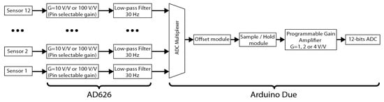
Figure 1.
Block diagram of the acquisition system.
The instrumental amplifier used in this design is the AD626 [43]. We have selected this amplifier due to the following characteristics:
- (1)
- It works with a single power supply. In our case, we supply the amplifier with the same voltage used for the Arduino Due, i.e., 3.3 V.
- (2)
- It allows voltage amplifications between 10 V/V (open circuit) and 100 V/V (short circuit) by using an external resistance, Rg.
- (3)
- It can accomplish the anti-aliasing filter function with just an external capacitor.
- (4)
- In single power supply mode, it presents low offset voltage (2.5 mV maximum), low voltage noise RTI (2 μV p-p), good CMRR (90 dB typical), and low power consumption (0.76 mW typical).
- (5)
- It is available in 8-Lead Plastic Mini-DIP package, which makes it easy to mount on a printed circuit board, even for an inexperienced person.
Figure 2 shows the circuit designed for the acquisition of the seismic noise. The signal provided by the sensor, i.e., the input signal, is a differential signal that swings between negative and positive values. With the AD626 working in single power supply mode, the negative signal would be cropped if the input signals were directly connected to the amplifier. In order to avoid this, an offset voltage is added to the input signal using a voltage divider. To allow the maximum possible swing of the signal, the offset has to be set up just in the middle of the input voltage range, between ground and the power supply, 3.3 V. For that, two equal resistances connected between 0 and 3.3 V will be enough to provide in the middle point the required 3.3/2 V. In our case, we have selected two resistances of 10 kΩ (with 0.1% of tolerance) as a compromise value. The parallel of these resistances with the internal resistance of the sensor (i.e., 5500 Ω for the Mark-L-4C3D and Mark-L-4C sensors [41]) has to be much lower than the internal resistance of the amplifier (200 kΩ). At the same time, the power consumed by these two resistances in series has to be as lower as possible.
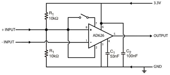
Figure 2.
Electronic schematic of the input stage.
It important to note that this offset voltage has to be considered as the new reference voltage or “ground” for the instrumental amplifier. Therefore, in this configuration pins 2 and 7 have to be connected also to the new reference voltage and not to 0 V.
The voltage gain is controlled through pin 7. In the proposed design, a jumper is used to configure the amplification to 10 V/V (open circuit) or 100 V/V (short circuit). Anyway, for our application purposes, an amplification of 10V/V (open circuit) is the most appropriate configuration.
The AD626 allows configuring a first order low pass filter just combining an internal resistance of 100 kΩ with an external capacitor, CF. In this way, the same device can be used simultaneously as amplifier and anti-aliasing filter, reducing the number of required components. In Figure 3, the resulting filter circuit is shown.
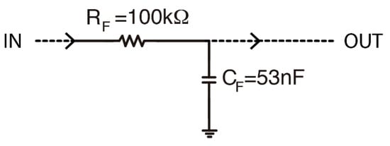
Figure 3.
First order low-pass filter.
For this kind of filter, the cutoff frequency is determined through the following equation:
Considering the minimum sampling frequency normally used (100 Hz) and the typical recorded frequencies of the seismic noise, the cutoff frequency has been configured to approximately 30 Hz. Therefore, by applying equation 1, it results an external capacitor of 53 nF.
Finally, the aim of the 100 nF capacitor, connected between the power supply and the ground, is to filter high-frequency electronic noise that might be interfering with the continuous voltage.
With all these considerations, the output signal of the AD626 is a common-mode signal, positive (with the middle voltage in 3.3/2 V), amplified by 10 V/V (or 100 V/V) and low-pass filtered (with a cutoff frequency of 30 Hz).
This output signal is directly connected to one analog input of the Arduino DUE, which is in charge of the programmable gain amplification and the digitization of the signal. The Arduino DUE board contains a 12-channel, 12-bit analog-to-digital converter, which allows to work with 12 analog inputs through a multiplexer. Thus, it reads analog signals between 0 and 3.3 V (the operating voltage) and converts them in a set of integer values between 0 and 4095, with a resolution of 0.8 millivolts per unit. The ADC can be configured in single ended or fully differential mode. In the fully differential mode, the number of input channels is reduced to 6. In the developed design, the ADC works in single ended mode, what allows the use of 12 analog inputs.
Previous to the analog-to-digital conversion, the ADC module of Arduino DUE contains a Programmable Gain Amplifier (PGA) and a Programmable Offset. For the single ended mode, the PGA can be set to gains of 1, 2, and 4. As the input signals are centered in Vcc/2 (i.e., 1.66 V) in the first stage, the Programmable Offset is not used in the proposed prototypes.
2.2. Control System
The control of the acquisition and recording processes is carried out through an Arduino Due board, which is in charge of performing the A/D conversion, the programmable voltage amplification, and the communication with Matlab, the SD shield, and the clock shield.
More specifically, the Arduino Due board carries out the following functions:
- Control the Programmable Voltage Gain.
- Convert the analog inputs to digital signals.
- Manage the communication with Matlab for configuration and real-time monitoring tasks.
- Send the registering data to the PC in real-time.
- Manage the recording of the data in the SD card.
- Retrieve the current date and hour from the clock shield.
- Manage the file name assigned automatically to the records (in plug and play mode).
To accomplish all these tasks, an Arduino sketch has been developed. A simplified flowchart of the acquisition process is shown in Figure 4.
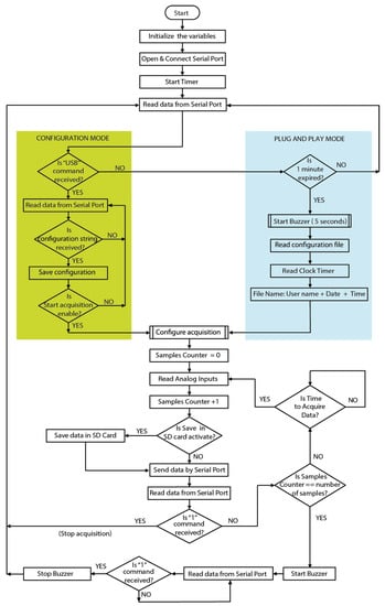
Figure 4.
Flowchart of the acquisition sketch.
Once the Arduino Due board is powered on, the sketch starts running. Firstly, the program variables are initialized and the serial port is opened. In this stage, two operation modes are possible: configuration, and plug and play modes, which are indicated in Figure 4 with green and blue shadows, respectively.
If during a specified period of time (i.e., 1 min), the Arduino Due receives the string command “USB” by serial port, it will know that it is connected to the PC via the Matlab interface and the system will enter in the configuration mode (see Section 2.2.1). In this operation mode, the Arduino Due will wait to receive from the GUI the appropriate parameter string (via the serial port) to save the configuration parameters in a file, named “Conf.txt”, and start the recording process.
On the contrary, if after a minute the string command “USB” was not received through the serial port, then the system would enter in the plug and play mode (see Section 2.2.2) and start recording data using the configuration parameters specified in the default configuration file (“Conf.txt”).
When acquisition parameters (see Section 2.2.1) are established, a counter of samples is initialized, sampling starts, and the time for the next sample is calculated. The number of samples to acquire and the selected analog inputs are indicated in the configuration parameters. The acquired data are recorded on the SD card (if this option is selected) and sent to the serial port. The part of the code corresponding to the acquisition of the analog signals, recording on the SD card and sending data via the serial port, takes an average time of 3 milliseconds for execution when all channels (i.e., 12) are registering and 0.75 milliseconds for recording three channels. The average time for saving one sample on SD card is 137 microseconds.
In the plug and play mode, the file name is assigned automatically. The program adds the current date and time, retrieved from an external clock device, to the file name, which is selected by the user and included in the configuration file. In this way, you can use the plug and play mode as many times as you want and each file will have a different name. Seismic data are saved in SAF format [44], i.e., in ASCII multi columns (with header). When the selected number of samples has been acquired, an external buzzer is activated to warn about the acquisition end. This is especially useful in the plug and play mode, where you only have to power off the system after acquisition. If the PC is connected to the Arduino Due (configuration mode), then the Matlab program will automatically send a string command “1” to stop the buzzer and a “USB” command to prepare the system for a new acquisition (See Supplementary Material).
The source code of the Arduino Due and Matlab programs, as well as an example of configuration file (ConF.txt) can be downloaded from:
2.2.1. Configuration Mode
If the acquisition system receives a “USB” command through the serial port during the first minute of power on, it will mean that the Arduino Due is connected to the PC through the USB cable and the Matlab application is running (configuration mode). In this situation, the user controls when to send the configuration parameters and to start with the data acquisition.
The configuration parameters are introduced through a GUI developed in Matlab. When the user decides, these parameters are sent to the Arduino Due and the acquisition stars. Once the configuration parameters are received by the Arduino Due, they are saved in an ASCII file named “ConF.txt”. In Table 1, the configuration parameters, as well as an example of the possible corresponding values, are shown.

Table 1.
Configuration parameters.
The parameters are sent and saved as a text string, with the different fields separated by spaces. Therefore, an example of configuration string could be the following one: “100 1 0.00080566 600 1 1 1 0 0 0 0 0 0 0 0 0 0 1Petrer_16Oct2018_105024;”.
The first field corresponds to the sampling frequency, which can be set to 100, 125, 200, 250 Hz. As Arduino Due uses a multiplexer to digitize the 12 channels, the sampling frequency and the maximum number of channels are directly related. In this sense, the higher number of channels is, the lower sampling frequency is going to be as well. Nevertheless, the minimum sampling frequency (100 Hz) is just the most common value and it allows working with the 12 analog inputs.
The second parameter is related with the programmable gain amplifier included in the Arduino Due board. It allows three different gains of 1, 2, and 4 V/V.
The next parameter provides the conversion of counts to volts. In the case of the Arduino Due, the maximum voltage is 3.3 V and the number of levels is 4096 (12 bits). These values are fixed to Arduino Due. Anyway, they are considered as parameters allowing the possibility of migration to other Arduino boards or the incorporation of an external analog-to-digital converter.
The fourth parameter corresponds to the number of samples. The minimum time is 1 min, and the maximum time depends only on the capacity of the SD card.
The next twelve characters are related with the twelve analog inputs, respectively, and they indicate which channels are used to acquire the data (set to “1”) and which ones are not (set to “0”). In this way, the Arduino Due will only acquire data from the selected channels and only these data will be sent through the serial port.
The next character is used to enable (“1”) or not (“0”) the recording of the acquired data in the SD card. As the data are sent via the serial port to the PC, the user can decide to save the data only in the computer.
After that, an additional character is used to indicate whether the acquisition must start immediately (“1”) or not (“0”). In fact, the user can send the configuration string to the Arduino DUE board in the stage previous to the field campaign. Thus, with the configuration file saved in the SD card, the developed acquisition system can be used in the plug and play mode as many times as the user wants, without needing any external computer to be connected.
Finally, a string of characters is added at the end with the name chosen for the data file. This name can be split in two parts: the first part corresponds to the name assigned by the user, meanwhile, the second part is assigned automatically with the current date and time of the computer.
2.2.2. Plug and Play Mode
In the plug and play mode, the user only has to power on the developed acquisition system to start recording. After the initial established time (1 min by default), the device automatically reads the configuration file (“ConF.txt”), where all the parameters related with the acquisition process are included (sampling frequency, duration, analog channels, etc.).
As mentioned in Section 2.2.1, the configuration file is saved in ASCII format. Therefore, it could also be created or modified manually using any text editor program. It is not mandatory to use the GUI developed in Matlab. This could be very useful if the user only wants to use the system in the plug and play mode, without real-time monitoring of the signals.
In this mode of operation, data are recorded in the SD card of the Arduino Due shield. The file name follows the structure indicated in the previous Section 2.2.1, so the current date and time obtained from the RTC are appended automatically to the end of the user selected file name. In this way, the developed system can work in plug and play mode as many times as the user wants, as each file will be saved with a different name. Also, the buzzer will sound during 5 seconds at the beginning of the acquisition, in order to let the user know that the system starts recording.
2.3. Hardware System
Figure 5 shows in detail the different blocks that compose the hardware system, as well as the different connections among them. Two different prototypes are presented, for three and twelve channels. The three-channel prototype is used for H/V measurements, where only one three-component sensor is needed. The twelve-channel prototype is used for array measurements, where several vertical sensors register seismic noise simultaneously.
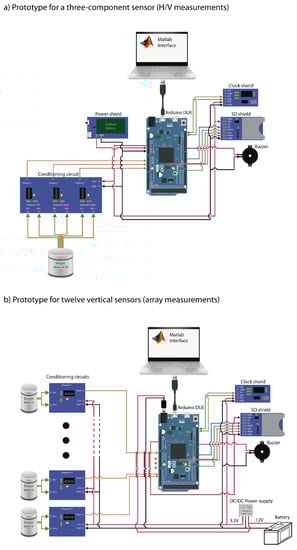
Figure 5.
Block diagram of the prototypes designed for (a) a three-component sensor and (b) for twelve vertical sensors.
In both prototypes, Arduino Due controls all the acquisition process (from the initialization of the variables to the data recording in the SD card). It is only connected to the computer in the configuration mode (see Section 2.2.1).
The Clock shield is the DS3231 [45]. This is a low-cost, highly accurate I2C real time clock (RTC), which works with a typical voltage of 3.3 V. It provides the current date and time to Arduino Due and it also includes a battery that maintains accurate timekeeping even when the main power is interrupted. The SD shield contains the SD card and it is used by Arduino Due to record all the acquired data. The buzzer is just connected to Arduino Due by one wire and it lets the user know when the acquisition has finished.
We have implemented two different conditioning circuit boards: for one and three input channels. The three-channel conditioning circuit has been designed as an Arduino Due shield, so it can be stacked together with the other commercial shields. The single-channel conditioning circuit has been designed as an independent board, which is connected with Arduino Due by wire. Twelve of them are used for the twelve-channel prototype. In this case, we have decided to implement each channel individually in order to provide more modularity and simplicity to the system, so that any conditioning circuit of one channel can be very easily replaced in case of failure.
The power supply is also different for both prototypes. In the case of the three-channel prototype, we have used a PowerBoost shield [46] with a Lithium ion 3.7 V 2050 mAh rechargeable battery (103456A-1S-3M model). The PowerBoost shield provides 5 V to Arduino Due, which converts it to 3.3 V supplying this new voltage to the rest of the circuits/shields of the system.
In the case of the twelve-channel prototype, if we followed the previous scheme, Arduino Due would have to feed the twelve conditioning circuits and the Clock and SD shields. That supposes four times higher demand of current with respect to the three-channel system. Therefore, we have opted for an external power supply, concretely a typically common 12 V battery. The Arduino Due is directly connected to the 12 V through the barrel jack connector. It converts this voltage into 3.3 V for internal use and for the SD shield. The 12 V battery is also connected to a fixed DC/DC module [47] that provides 3.3 V to the twelve conditioning circuits and the Clock shield. The use of this battery is not mandatory; we have selected it because is the battery usually used the most in this type of systems. Input voltage recommended for Arduino Due board is in the range of 7–12 V and for DC/DC module is in the range of 6–28V. Thus, any battery between 7 and 12 V could be used, even a power bank that is usually used to charge mobile phones could be used. Our experience with a 12 V 4.0 AH (amp hour) full charged battery is that the system could be recording in continuous mode around 130 hours (i.e., more than 5 days).
In Figure 6, we show in a picture how the different modules are arranged for both prototypes.
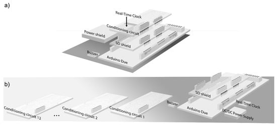
Figure 6.
Arrangement of the different hardware modules for both prototypes, with (a) three channels and (b) twelve channels.
2.4. Graphical Interface in Matlab
Figure 7 shows the Matlab-based GUI of the developed acquisition system, which is used for configuration of the Arduino Due and for real-time monitoring of the registered signals. The GUI has been designed using Matlab 8.4.0 (Release 2014b) and has been tested with this and other later versions under the operating systems of MacOs X and Windows.
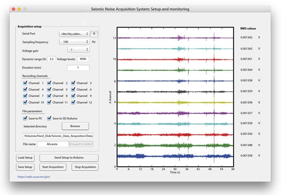
Figure 7.
GUI (graphical user interface) of the seismic data acquisition system.
When the program starts, it automatically loads the latest configuration parameters, saved in the file “current_status.mat”. The configuration is divided in four main blocks. The first one is related with the serial port that connects with the Arduino Due. By default, the selected option is “None”, but once the Arduino Due is connected to the computer, the associated serial port will be available. The button “R”, located on the right side, allows refreshing the available serial ports.
In the second block, the parameters related with the acquisition and the analog-to-digital converter are introduced. That is the sampling frequency; the voltage gain (corresponding to the PGA of the Arduino Due); the dynamic range and the voltage levels (both dependents on the ADC used); and the acquisition time. Besides this, the input analog channels are selected individually from 1 to 12. For the H/V measurements prototype, channels 2, 4, and 6 have to be chosen (see the block diagram in Figure 5a). However, for the array measurements prototype, up to a total of 12 channels can be selected, depending on the number of available sensors.
The third block comprises to the data recording configuration. The user can select either to save the registered data in the SD card of Arduino Due or in the computer. Any of these options, both, or none can be chosen. In the case of saving the data on the PC, the destination directory and the user selected file name must be also introduced. The current date and time are automatically appended to the user selected file name.
Finally, there are five buttons located at the bottom of the interface. In the left side, we have two buttons to load and save the configuration parameters. Once the configuration is prepared, we can only send the configuration file to the Arduino Due (“Send Setup to Arduino” button) or send it and start immediately the data acquisition (“Start acquisition” button). In both cases, the configuration file is saved on the SD card, leaving the Arduino Due ready to work in the plug and play mode. During the acquisition process, all the options remain locked except the “Stop acquisition” button, which allows interrupting the data acquisition and returning to the initial state (unlocking again all the options).
Once starting the data acquisition through the GUI, the interface shows on the right side the registered signals in real-time. Specifically, the twelve acquisition channels are displayed second by second, in 10-second windows. Together with the graphical representation of each of the signals, the RMS value is also shown. Thus, any error in any of the registration channels might be detected immediately. At the end of the data acquisition period, the complete records are displayed (Figure 7).
3. Results and Discussion
As a result of this work, two prototypes have been designed and implemented for seismic noise measurements. One of the prototypes has been optimized to work with three-component sensors (Figure 8) and take H/V measurements. Meanwhile, the other one has been designed to work with a maximum of twelve vertical sensors (Figure 9) and take array measurements.
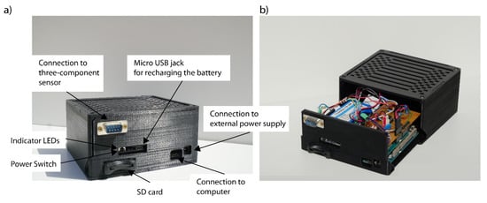
Figure 8.
Prototype designed for three-component sensors (H/V measurements). (a) System enclosure with indications about input connections and (b) component distribution inside the enclosure.
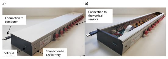
Figure 9.
Prototype designed for twelve vertical sensors (array measurements. (a) System enclosure with indications about input connections and (b) component distribution inside the enclosure.
The three-component data acquisition system is integrated in a small box of dimensions 130 × 120 × 65 mm. It includes a Lithium ion 3.7 V 2050 mAh battery that can be recharged through the Micro USB jack shown in Figure 8. The power switch activates the plug and play mode. When the system is connected to the computer (i.e., for configuration or monitoring purposes), it does not require switching on the battery.
The twelve-channel data acquisition system is included in a box of dimensions 1070 × 150 × 60 mm. In this case, the modularity and simplicity of the system have prevailed above the maximum possible integration of the components. In this way, the conditioning circuit of each channel is designed on a different board and it can be easily replaced in case of failure (Figure 9). Whether the system is connected to the computer or not, it requires an external power supply to provide the necessary voltage to the conditioning circuits of each channel.
Before evaluating the performance of both devices in real situations, they have been characterized in the laboratory by using sine waves of known frequency and amplitude. The Tektronix AFG310 function generator has been used to provide sine waves of 50 mV amplitude and frequencies between 1 and 50 Hz. In order to test the gain of 100 with the AD626, a voltage divider has been used in order to reduce the amplitude of the input signal and to not saturate the recorded signal.
In Table 2, the obtained experimental results are presented together with the corresponding theoretical values. For all the stages and amplifications, the voltage gains present a good agreement. In the case of the cutoff frequency of the low-pass filter, the differences are due to the tolerance of the components. This frequency is inversely proportional to the RC time constant (Equation (1)), whose experimental and theoretical values are 5.3 and 6.6 milliseconds, respectively. The AD626 on-chip resistors have an absolute tolerance of ±20% [43] and the external capacitor has a tolerance of ±20%, which means that the differences obtained in the RC time constant are within the expected margin of error. Anyway, the obtained cutoff frequency is still far above the frequencies of interest of the seismic noise.
Table 2.
Operating characteristics of the designed acquisition system
Respecting the power consumption, both prototypes consume almost the same: 1.05 ± 0.02 and 1.13 ± 0.02 W for the three-component and the twelve-channel devices, respectively. It means that the consumption of the conditioning circuits is much lower than the one of the other components (e.g., Arduino Due, SD shield, etc.).
The sensitivity of the developed system (Table 3) has been calculated following the process established in a previous Instrument Workshop: Site Effect Assessment Using Ambient Excitations [48]. Three experimental measurements have been carried out with the inputs of the twelve channels connected to 0 V, +1 V (normal polarity) and −1 V (inverse polarity). The output voltage was recorded during 1 min at the sampling frequency of 100 Hz, and subsequently analyzed to obtain the sensitivity and the relative error. From Table 3, we can observe that the relative error is below 1.2%, which is quite an acceptable value. In the mentioned Workshop, the relative error obtained for 12 analyzed commercial recorders was between 0.03% and 7.71%. Besides this, the obtained results state that the polarity does not affect the sensitivity of the system and that the twelve analyzed channels have very similar sensitivity.
Table 3.
Sensitivity of the designed acquisition system.
3.1. Field Test with the Three-Component Acquisition System
To test the suitability of the developed three-component acquisition system for recording seismic noise, H/V measurements were carried out in two different sites where H/V studies had been carried out previously using a commercial 24-bits digitizer, Reftek. The selected test sites were chosen along the province of Alicante (southeast Spain): Almoradí (−0.7829°, 38.1118°) and Catral (−0.8260°, 38.1520°).
In both sites, 30 min were registered with a sampling frequency of 100 Hz. The voltage gain of the AD626 amplifier and the Arduino Due was 10 and 1, respectively. The unity gain was used for the Reftek.
Three-component sensors (Mark L-4C-3D), with a natural frequency of 1 Hz, were used for registering with both acquisition systems. Despite being their natural frequency of 1 Hz, these sensors allow retrieving resonant frequencies up to 0.2 Hz, as it is shown in the works of Strollo et al. [49,50].
In Figure 10, the results obtained using the developed system (right column) and the Reftek (left column) are shown. In the case of Almoradí site, the H/V results obtained with the designed prototype have been compared with the ones obtained using the Reftek in two different time periods: February 2017 and March 2017. In the case of Catral, the measures with the Reftek equipment were carried out in 2017. Although the noise characteristics (i.e., amplitude spectra and locations of dominant sources) may be different in each of the time periods, the H/V curves at a particular site are time stable and mainly determined by the soil characteristics [12,51,52]. In this sense, we can observe some amplitude differences among the H/V curves, even when the same recorder is used (e.g., measures taken in Almoradí site with the same Reftek recorder in February and March), but the observed peaks remain approximately at the same frequencies. It is important to highlight that the observed H/V peaks are directly related with the resonant frequencies of the soil under study [10,11], so they constitute the characteristics to be determined. Therefore, the differences observed in the amplitude of the H/V peaks do not influence the estimation of the site amplification factor, as it is established for many authors [53,54,55,56,57].
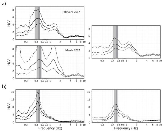
Figure 10.
H/V curves estimated for (a) Almoradí and (b) Catral using the Reftek (left column) and the developed acquisition system (right column).
We have recently used the developed system to perform microzonation studies in two cities of the province of Alicante and to estimate the resonant frequency in some of their buildings.
3.2. Field Test with the 12-Channel Acquisition System
To assess the suitability of the 12-channel acquisition system for seismic noise array measurements, real surveys were deployed in two different sites along the province of Alicante (southeast Spain). For comparison purposes, we selected two sites where array studies had been carried out previously using commercial instruments: Almoradí (−0.7829°, 38.1118°) and Rojales (−0.7202°, 38.0912°).
In Almoradí site, a circular layout of 40 m of diameter was deployed with twelve 1 Hz vertical sensors (Mark L4) distributed around the circumference. In 2011, array measurements were taken in the same site using as digitizers the 24-bit Earth Data pr6-24 portable model [58]. In this study, two circular arrays of apertures 25 and 100 m were deployed. Nine Mark L4 sensors were used for each array, with one of them in the center of the circular layout and the other eight distributed around it. In Figure 11a (left column) the geometries used with both instruments are shown.
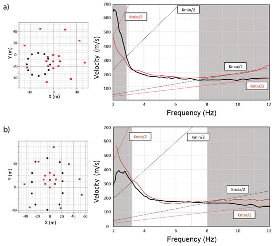
Figure 11.
Array geometries (left column) and estimated dispersion curves (right column) for the developed data acquisition system (black color) and the commercial equipment (red color), for the sites under study: (a) Almoradí, and (b) Rojales. Wavenumber limits (kmax/2 and kmin/2) are represented with dashed lines in the corresponding color.
In Rojales site, an ellipsoidal array was implemented, with semi-major and semi-minor axes equal to 45 and 26 m, respectively (Figure 11b, left column). This geometry was imposed by the urban conditions, different from those in 2011. Twelve 1 Hz vertical sensors (Mark L4) were distributed around the ellipse. In 2011, a wider free area was available. Thus, a circular array of 25 m diameter and a polygonal array with a maximum distance between stations around 100 m were deployed [59] (Figure 11b, left column). In this site, 24-bit Earth Data pr6-24 portable model digitizers and nine Mark L4 sensors were used for both arrays (in 2011).
The aperture of the array and the number of sensors determine the theoretical array response and the measurement limits in terms of the wavenumber, k. In this way, the maximum resolution of the array depends on the minimum detectable wavenumber, i.e., kmin/2. While the maximum reliable wavenumber, i.e., kmax/2, is limited by the aliasing effect. In the case of the array measurements taken in 2011, both arrays were combined, widening the range of the wavenumber values. In Table 4, the theoretical wavenumber limits associated to the commented geometries are presented.
Table 4.
Theoretical wavenumber limits (rad/m) for the different geometries used.
All the array measurements, with both instruments, were configured with a recording time of 30 min and a sampling frequency of 100 Hz. In the case of the developed acquisition system, the voltage gain of the AD626 amplifier and the Arduino Due was set up to 10 and 1, respectively.
The recorded signals have been analyzed with the f-k method, using the Geopsy software [60] and applying the same configuration parameters used in the previous studies [59]. As result of the f-k method analysis, the velocity of the surface waves as a function of the frequency (i.e., the dispersion curve) has been estimated. The comparison with the dispersion curves estimated in 2011 is possible based on the assumption of a stochastic wavefield, which is stationary both in time and space [12]. The temporal consistency and the repeatability of the array analyses are demonstrated in several works (e.g., Endrun et al. [51] and Rosa-Cintas et al. [52]).
In Figure 11a (right column), the dispersion curves obtained for the Almoradí site, together with the theoretical wavenumber limits, are shown. The gray shaded area corresponds to the frequencies that are outside of the valid frequency range associated to the implemented array. The intersection of the theoretical wavenumber limits and the experimental dispersion curve provides the valid frequency range for each case. From the obtained results, we can observe the good agreement between both dispersion curves in the frequency range of 2.9 to 7.5 Hz, which is the useful frequency range associated to the array deployed with the developed acquisition system. Therefore, information observed out of this range should not be considered because it is out of the resolution of the implemented array.
In the case of Rojales site (Figure 11b, right column), the valid frequency range associate to the array deployed with the proposed acquisition system is between 3.2 and 8 Hz. In this frequency range, we can observe that both curves present a good correlation between them.
From the obtained results, we can observe the suitability of the developed acquisition system for array measurements, providing practically the same results that the ones obtained with other commercial equipment.
We have recently used this multi-channel data acquisition system to perform array measurements in seismic-induced landslides in order to estimate their structure and the characteristics of the corresponding materials.
4. Conclusions
In this paper, two multi-channel data acquisition systems have been developed and implemented for registering seismic noise. One of them, a three-channel prototype, has been optimized for working with three-component sensors, and the other one, a twelve-channel prototype, has been designed for working with twelve vertical geophones. They are directly applied for taking H/V and array measurements, respectively, what allow estimating the soil characteristics.
A conditioning signal circuit has been designed to amplify and filter the input analog signals. Two different implementations have been carried out, with three and one input channel. The first one has been designed as an Arduino Due shield, so that it can be stacked on the Arduino board as one more shield. The other one, the one-channel conditioning circuit, is connected with the Arduino Due by wire. Therefore, twelve of them are used for the twelve-channel prototype. This implementation provides more modularity and simplicity to the system, so that any conditioning circuit of one channel can be very easily replaced in case of any malfunction.
The data acquisition is controlled completely by the Arduino Due, which can register automatically by just switching it on (plug and play mode). Both prototypes are battery powered, so they do not need any external computer. The graphical user-friendly interface developed in Matlab is used for the configuration of the control system and for the real-time visualization of all the signals, when it is required.
The real-time monitoring shows the input signals and their respective RMS value, what allows detecting any anomaly in any of the registration channels immediately, in order to correct it as soon as possible.
The most important benefit is to make a system accessible to any research group, but especially to those with less economic resources, so that it allows them to conduct studies based on seismic noise measurements for soil characterization and seismic hazard estimation. With this objective, the developed designs are open-hardware, open-software, easy to implement (both assembly and component level), and low-cost.
Supplementary Materials
The following are attached to this article: Source code of the Arduino Due and Matlab programs; and an example of a configuration file (ConF.txt). Also it is available online at https://github.com/JLSolerLlorens/Plug-and-Play-System-for-Seismic-Noise-Measurements. (Also available at https://www.mdpi.com/2079-9292/8/9/1035/s1)
Author Contributions
Conceptualization, J.L.S.-L. and J.J.G.-M.; Data curation, J.L.S.-L., J.J.G.-M., B.Y.N.-B. and J.J.G.-C.; Formal analysis, S.R.-C.; Funding acquisition, J.J.G.-M.; Investigation, J.L.S.-L., J.J.G.-M., B.Y.N.-B., S.R.-C. and J.J.G.-C.; Methodology, J.J.G.-M.; Project administration, J.J.G.-C.; Resources, B.Y.N.-B. and J.O.Z.; Software, J.L.S.-L.; Supervision, J.J.G.-M., S.R.-C. and J.J.G.-C.; Validation, J.L.S.-L. and S.R.-C.; Visualization, J.J.G.-M., S.R.-C. and J.O.Z.; Writing–original draft, J.L.S.-L. and J.J.G.-M.; Writing–review & editing, J.J.G.-M., B.Y.N.-B., S.R.-C., J.O.Z. and J.J.G.-C.
Funding
This research was funded by the Ministerio de Economia, Industria y Competitividad (grant number CGL2016-77688-R AEI/FEDER, UE); Spanish MINECO and European funds under project EPILATES (grant number CGL2015.65602-R); and Regional Government of Comunidad Valenciana (Spain) (grant number AICO/2016/098).
Acknowledgments
We thank to the Institut Cartogràfic i Geològic de Catalunya (ICGC) that provided us the Mark L4 sensors for the development of this work. We are very thankful to Victor Navarro Fuster for their collaboration in the assembly of the equipment. We also want to thank Julio Rosa Herranz for their comments and suggestions. Finally, we are very grateful to the assistant editor, Xenia Xie, and the anonymous rewiewers for their comments and suggestions, which helped us to clarify and improve the original manuscript.
Conflicts of Interest
The authors declare no conflict of interest. The funders had no role in the design of the study; in the collection, analyses, or interpretation of data; in the writing of the manuscript, or in the decision to publish the results. The identification of the name of the instruments’ manufacturers does not mean any endorsement of their products.
References
- Hutt, C.R.; Evans, J.R.; Followill, F.; Nigbor, R.L.; Wielandt, E. Guidelines for Standardized Testing of Broadband Seismometers and Accelerometers; Open-File Report 2009-1295; U.S. Geological Survey: Reston, VA, USA, 2010.
- Asten, M.W. Geological control of the three-component spectra of Rayleigh-wave microseisms. Bull. Seismol. Soc. Am. 1978, 68, 1623–1636. [Google Scholar]
- Gutenberg, B. Microseisms. Adv. Geophys. 1958, 5, 53–92. [Google Scholar]
- Bonnefoy-Claudet, S.; Cotton, F.; Bard, P.-Y. The nature of the seismic noise wave field and its implication for site effects studies: A literature review. Earth Sci. Rev. 2006, 79, 205–227. [Google Scholar] [CrossRef]
- Acerra, C.; Alguacil, G.; Atakan, K.; Azzara, R.M.; Bard, P.-Y.; Blarel, F.; Borges, A.; Cara, F.; Teves-Costa, P.; Duval, A.-M.; et al. Sesame Project—Deliverable D01-02—WP02: Controlled Instrumental Specifications—Final Report of the Instrument Workshop 22–26 October 2001; University of Bergen: Bergen, Norway, 2002. [Google Scholar]
- Guillier, B.; Atakan, K.; Chatelain, J.L.; Havskov, J.; Ohrnberger, M.; Cara, F.; Duval, A.M.; Zacharopoulos, S.; Teves-Costa, P.; The SESAME Team. Influence of instruments on the H/V spectral ratios of ambient vibrations. Bull. Earthq. Eng. 2008, 6, 3–31. [Google Scholar] [CrossRef]
- Nakamura, Y. A method for dynamic characteristics estimation of subsurface using microtremors on the ground surface. Q. Rep. Railw. Tech. Res. Inst. Jpn. 1989, 30, 25–33. [Google Scholar]
- Field, E.H.; Jacob, K. The theoretical response of sedimentary layers to ambient seismic noise. Geophys. Res. Lett. 1993, 20–24, 2925–2928. [Google Scholar] [CrossRef]
- Lermo, J.; Chávez-García, F.J. Are microtremors useful in site response evaluation? Bull. Seismol. Soc. Am. 1994, 84, 1350–1364. [Google Scholar]
- Bonnefoy-Claudet, S.; Köhler, A.; Cornou, C.; Wathelet, M.; Bard, P.-Y. Effects of love waves on microtremor H/V ratio. Bull. Seismol. Soc. Am. 2008, 98, 288–300. [Google Scholar] [CrossRef]
- Rosa-Cintas, S.; Galiana-Merino, J.J.; Rosa-Herranz, J.; Molina, S.; Martínez-Esplá, J.J. Polarization analysis in the stationary wavelet packet domain: Application to HVSR method. Soil Dyn. Earthq. Eng. 2012, 42, 246–254. [Google Scholar] [CrossRef]
- Aki, K. Space and time spectra of stationary stochastic waves, with special reference to microtremors. Bull. Earthq. Res. Inst. Tokyo Univ. 1957, 25, 415–457. [Google Scholar]
- Ohori, M.; Nobata, A.; Wakamatsu, K. A comparison of ESAC and FK methods of estimating phase velocity using arbitrarily shaped microtremor analysis. Bull. Seismol. Soc. Am. 2002, 92, 2323–2332. [Google Scholar] [CrossRef]
- Okada, H.; Suto, K. The Microtremor Survey Method; Geophysical Monograph Series 12; Asten, M.W., Ed.; Society of Exploration Geophysicists: Tulsa, Oklahoma, 2003. [Google Scholar]
- Ling, S.; Okada, H. An extended use of the spatial autocorrelation method for the estimation of geological structure using microtremors. In Proceedings of the 89th SEGJ Conference, Nagoya, Japan, October 12–14 1993; pp. 44–48. (In Japanese). [Google Scholar]
- Capon, J. High-resolution frequency-wavenumber spectrum analysis. Proc. IEEE 1969, 57, 1408–1418. [Google Scholar] [CrossRef]
- Lacoss, R.T.; Kelly, E.J.; Toksöz, M.N. Estimation of seismic noise structure using array. Geophysics 1969, 34, 21–38. [Google Scholar] [CrossRef]
- Asten, M.W.; Henstridge, J.D. Array estimators and use of microseisms for reconnaissance of sedimentary basins. Geophysics 1984, 49, 1828–1837. [Google Scholar] [CrossRef]
- Xia, J.; Miller, R.D.; Park, C.B. Estimation of near-surface shear-wave velocity by inversion of Rayleigh waves. Geophysics 1999, 64, 691–700. [Google Scholar] [CrossRef]
- Ohrnberger, M.; Scherbaum, F.; Krüger, F.; Pelzing, R.; Reamer, S.K. How good are shear-wave velocity models obtained from inversion of ambient vibrations in the lower Rhine embayment (N.W. Germany). Boll. Geofis. Teor. Appl. 2004, 45, 215–232. [Google Scholar]
- Parolai, S.; Mucciarelli, M.; Gallipoli, M.R.; Richwalski, S.M.; Strollo, A. Comparison of empirical and numerical site responses at the Tito Test Site, Southern Italy. Bull. Seismol. Soc. Am. 2007, 97, 1413–1431. [Google Scholar] [CrossRef]
- Mahajan, A.K.; Galiana-Merino, J.J.; Lindholm, C.; Arora, B.R.; Mundepi, A.K.; Nitesh, R.; Neetu, C. Characterization of the sedimentary cover at the Himalayan foothills using active and passive seismic techniques. J. Appl. Geophys. 2011, 73, 196–206. [Google Scholar] [CrossRef]
- NEHRP 2015. Recommended Seismic Provisions for New Buildings and other Structures; FEMA P-1050; Federal Emergency Management Agency: New York, NY, USA, 2015.
- Saraò, A.; Clocchiatti, M.; Barnaba, C.; Zuliani, D. Using an Arduino seismograph to raise awareness of earthquake hazard through a multidisciplinary approach. Seismol. Res. Lett. 2016, 87, 186–192. [Google Scholar] [CrossRef][Green Version]
- Soler-Llorens, J.L.; Galiana-Merino, J.J.; Giner-Caturla, J.; Jauregui-Eslava, P.; Rosa-Cintas, S.; Rosa-Herranz, J. Development and programming of Geophonino: A low cost Arduino-based seismic recorder for vertical geophones. Comput. Geosci. 2016, 94, 1–10. [Google Scholar] [CrossRef]
- Soler-Llorens, J.L.; Galiana-Merino, J.J.; Giner-Caturla, J.J.; Jauregui-Eslava, P.; Rosa-Cintas, S.; Rosa-Herranz, J.; Nassim Benabdeloued, B.Y. Design and test of Geophonino-3D: A low-cost three-component seismic noise recorder for the application of the H/V method. Sens. Actuators A Phys. 2018, 269, 342–354. [Google Scholar] [CrossRef]
- Picozzi, M.; Milkereit, C.; Parolai, S.; Jaeckel, K.H.; Veit, I.; Fischer, J.; Zschau, J. GFZ wireless seismic array (GFZ-WISE), a wireless mesh network of seismic sensors: New perspectives for seismic noise array investigations and site monitoring. Sensors 2010, 10, 3280–3304. [Google Scholar] [CrossRef] [PubMed]
- Fischer, J.; Redlich, J.P.; Zschau, J.; Milkereit, C.; Picozzi, M.; Fleming, K.; Brumbulli, M.; Lichtblau, B.; Eveslage, I. A wireless mesh sensing network for early warning. J. Netw. Comput. Appl. 2012, 35, 538–547. [Google Scholar] [CrossRef]
- Dai, K.; Li, X.; Lu, C.; You, Q.; Huang, Z.; Wu, H.F. A low-cost energy-efficient cableless geophone unit for passive surface wave surveys. Sensors 2015, 15, 24698–24715. [Google Scholar] [CrossRef] [PubMed]
- Jamali-Rad, H.; Campman, X. Internet of things-based wireless networking for seismic applications. Geophys. Prospect. 2018, 66, 833–853. [Google Scholar] [CrossRef]
- Boxberger, T.; Fleming, K.; Pittore, M.; Parolai, S.; Pilz, M.; Mikulla, S. The multi-parameter wireless sensing system (MPwise): Its description and application to earthquake risk mitigation. Sensors 2017, 17, 2400. [Google Scholar] [CrossRef] [PubMed]
- Tian, R.; Wang, L.; Zhou, X.; Xu, H.; Lin, J.; Zhang, L.; Tian, R.; Wang, L.; Zhou, X.; Xu, H.; et al. An integrated energy-efficient wireless sensor node for the microtremor survey method. Sensors 2019, 19, 544. [Google Scholar] [CrossRef]
- Polo, A.; Narvaez, P.; Robles Algarín, C. Implementation of a cost-effective didactic prototype for the acquisition of biomedical signals. Electronics 2018, 7, 77. [Google Scholar] [CrossRef]
- Mumtaz, Z.; Ullah, S.; Ilyas, Z.; Aslam, N.; Iqbal, S.; Liu, S.; Meo, J.A.; Madni, H.A. An automation system for controlling streetlights and monitoring objects using Arduino. Sensors 2018, 18, 3178. [Google Scholar] [CrossRef]
- Costa, D.G.; Duran-Faundez, C. Open-source electronics platforms as enabling technologies for smart cities: Recent developments and perspectives. Electronics 2018, 7, 404. [Google Scholar] [CrossRef]
- Garcia-Breijo, E.; Garrigues, J.; Sanchez, L.G.; Laguarda-Miro, N. An embedded simplified fuzzy artmap implemented on a microcontroller for food classification. Sensors 2013, 13, 10418–10429. [Google Scholar] [CrossRef] [PubMed]
- Robles-Algarín, C.; Echavez, W.; Polo, A. Printed circuit board drilling machine using recyclables. Electronics 2018, 7, 240. [Google Scholar] [CrossRef]
- Pantoli, L.; Muttillo, M.; Ferri, G.; Stornelli, V.; Alaggio, R.; Vettori, D.; Chinzari, L.; Chinzari, F. Electronic system for structural and environmental building monitoring. In Lecture Notes in Electrical Engineering; Springer: Cham, Switzerland, 2019; Volume 539, pp. 481–488. [Google Scholar]
- Muttillo, M.; Di Battista, L.; de Rubeis, T.; Nardi, I. Structural health continuous monitoring of buildings—A modal parameters identification system. In Proceedings of the 2019 4th International Conference on Smart and Sustainable Technologies (SpliTech), Split, Croatia, 12–21 June 2019; pp. 1–4. [Google Scholar]
- Barile, G.; Leoni, A.; Pantoli, L.; Stornelli, V. Real-time autonomous system for structural and environmental monitoring of dynamic events. Electronics 2018, 7, 420. [Google Scholar] [CrossRef]
- Havskov, J.; Alguacil, G. Instrumentation in Earthquake Seismology, 2nd ed.; Springer: Cham, Switzerland, 2016; p. 70. [Google Scholar]
- Guidelines for the Implementation of the H/V Spectral Ratio Technique on Ambient Vibrations. SESAME European Research Project, Deliverable D23.12 (WP12). Available online: Ftp://ftp.geo.uib.no/pub/seismo/SOFTWARE/SESAME/USER-GUIDELINES/SESAME-HV-User-Guidelines.pdf (accessed on 09 August 2019).
- Analog Devices. Available online: https://www.analog.com/media/en/technical-documentation/data-sheets/AD626.pdf (accessed on 10 August 2019).
- H/V Technique: Data Processing. SESAME European Research Project, Deliverable D09.03 (WP03). Available online: http://sesame.geopsy.org/Delivrables/D09-03_Texte.pdf (accessed on 10 August 2019).
- Maxim Integrated. Available online: https://datasheets.maximintegrated.com/en/ds/DS3231.pdf (accessed on 10 August 2019).
- Adafruit PowerBoost 500 Shield. Available online: https://learn.adafruit.com/adafruit-powerboost-500-shield-rechargeable-battery-pack (accessed on 10 August 2019).
- Würth Elektronik. Available online: https://katalog.we-online.de/pm/datasheet/173950378.pdf (accessed on 10 August 2019).
- Controlled Instrumental Specifications. SESAME European Research Project, Deliverable D01.02 (WP02). Available online: http://sesame.geopsy.org/Delivrables/D01-02_Texte.pdf (accessed on 5 September 2019).
- Strollo, A.; Bindi, D.; Parolai, S.; Jäckel, K.H. On the suitability of 1s geophone for ambient noise measurements in the 0.1–20 Hz frequency range: Experimental outcomes. Bull. Seismol. Soc. Am. 2008, 6, 141–147. [Google Scholar] [CrossRef]
- Strollo, A.; Parolai, S.; Jäckel, K.H.; Marzorati, S.; Bindi, D. Suitability of short-period sensors for retrieving reliable H/V peaks for frequencies less than 1 Hz. Bull. Seismol. Soc. Am. 2008, 98, 671–681. [Google Scholar] [CrossRef]
- Endrun, B.; Ohrnberger, M.; Savvaidis, A. On the repeatability and consistency of three-component ambient vibration array measurements. Bull. Earthq. Eng. 2010, 8, 535–570. [Google Scholar] [CrossRef]
- Rosa-Cintas, S.; Galiana-Merino, J.J.; Rosa-Herranz, J.; Molina, S.; Giner-Caturla, J. Suitability of 10 Hz vertical geophones for seismic noise array measurements based on frequency-wavenumber and extended spatial autocorrelation analyses. Geophys. Prospect. 2013, 61, 183–198. [Google Scholar] [CrossRef]
- Lachet, C.; Bard, P.-Y. Numerical and theoretical investigations on the possibilities and limitations of nakamura’s technique. J. Phys. Earth 1994, 42, 377–397. [Google Scholar] [CrossRef]
- Bard, P.-Y. Microtremor Measurement: A Tool for Site Effect Estimation? Irikura, K., Kudo, K., Okada, H., Sasatami, T., Eds.; CRC Press: Boca Raton, FL, USA, 1998; pp. 1251–1279. [Google Scholar]
- Fäh, D.; Kind, F.; Giardini, D. A theoretical investigation of average H/V ratios. Geophys. J. Int. 2001, 145, 535–549. [Google Scholar] [CrossRef]
- Arai, H.; Tokimatsu, K. S-wave velocity profiling by inversion of microtremor H/V spectrum. Bull. Seismol. Soc. Am. 2004, 94, 53–63. [Google Scholar] [CrossRef]
- Bonnefoy-Claudet, S.; Cornou, C.; Bard, P.-Y.; Cotton, F.; Moczo, P.; Kristek, J.; Fäh, D. H/V ratio: A tool for site effects evaluation. Results from 1-D noise simulations. Geophys. J. Int. 2006, 167, 827–837. [Google Scholar] [CrossRef]
- Earth Data—PR6-24 Specification. Available online: http://www.earthdata.co.uk/pr6-24sp.html (accessed on 10 August 2019).
- Rosa-Cintas, S.; Galiana-Merino, J.J.; Molina-Palacios, S.; Rosa-Herranz, J.; García-Fernández, M.; Jiménez, M.J. Soil characterization in urban areas of the Bajo Segura Basin (Southeast Spain) using H/V, F–K and ESAC methods. J. Appl. Geophys. 2011, 75, 543–557. [Google Scholar] [CrossRef]
- Geopsy Software. Available online: http://www.geopsy.org/download.php (accessed on 10 August 2019).


© 2019 by the authors. Licensee MDPI, Basel, Switzerland. This article is an open access article distributed under the terms and conditions of the Creative Commons Attribution (CC BY) license (http://creativecommons.org/licenses/by/4.0/).