Abstract
With the emergence of small cell networks and fifth-generation (5G) wireless networks, the backhaul becomes increasingly complex. This study addresses the problem of how a central SDN orchestrator can flexibly share the total backhaul capacity of the various wireless operators among their gateways and radio nodes (e.g., LTE enhanced Node Bs or Wi-Fi access points). In order to address this backhaul resource allocation problem, we introduce a novel backhaul optimization methodology in the context of the recently proposed LayBack SDN backhaul architecture. In particular, we explore the decomposition of the central optimization problem into a layered dual decomposition model that matches the architectural layers of the LayBack backhaul architecture. In order to promote scalability and responsiveness, we employ different timescales, i.e., fast timescales at the radio nodes and slower timescales in the higher LayBack layers that are closer to the central SDN orchestrator. We numerically evaluate the scalable layered optimization for a specific case of the LayBack backhaul architecture with four layers, namely a radio node (eNB) layer, a gateway layer, an operator layer, and central coordination in an SDN orchestrator layer. The coordinated sharing of the total backhaul capacity among multiple operators lowers the queue lengths compared to the conventional backhaul without sharing among operators.
1. Introduction
1.1. Motivation
In conventional wireless networks, each wireless service operator maintains its own wireless network infrastructure with its own backhaul network that interconnects the wireless network frontend with the Internet at large. Typically, each operator has a fixed maximum installed backhaul capacity. Sudden demand surges for backhaul capacity from the wireless devices and the corresponding radio nodes, e.g., the LTE enhanced Node Bs (eNBs) and Wi-Fi access points (APs), of one operator may overwhelm the operator’s backhaul capacity and result in poor service quality, and ultimately, reduced revenue. Overall, with the advances in the wireless transmission capacities, the backhaul has emerged as a critical bottleneck of novel high-capacity wireless networks, such as small cell networks and 5G networks [1,2,3,4,5,6,7].
Recently, Software-Defined Networking (SDN)-based backhaul architectures have been proposed to flexibly interconnect the backhaul networks of the different operators in a centrally controlled manner, as reviewed in detail in Section 2. The central SDN control enables the dynamic on-demand sharing of the backhaul resources among the various operators. Thus, sudden demand surges for backhaul capacity from the radio nodes (e.g., LTE eNBs and Wi-Fi APs) of one operator may be served by sharing the backhaul capacities of the various operators. Of course, aside from the technical capabilities, appropriate legal and business agreements need to be in place between the operators to make the sharing practically feasible and economically advantageous.
The SDN-based control of the backhaul resource sharing poses two main challenges. First, the aggregate of multiple operator networks with all their radio nodes and subscribing wireless devices considered by the central SDN orchestrator can be very large; thus posing scalability challenges. Second, the central SDN orchestrator that coordinates among multiple operators may be far removed from the distributed radio nodes resulting in long signaling delays and accordingly slow reactions to dynamic demand variations at the radio nodes. Thus, purely centralized optimization is not practical for backhaul networks. Rather, distributed optimization strategies are needed for operating large backhaul networks.
Network optimization that operates on distributed systems has so far had two flavors: peer-to-peer optimization for a flat (i.e., not layered) system and Network Utility Maximization (NUM) [8,9,10,11] which employs dual decomposition to distribute computations across different terminals that share the network resources. The dual decomposition leads to a master-slave model, where each user (slave) needs to directly interact with the SDN controller (master). The main benefit of operating the NUM is that the SDN controller simply passes the dual variable iterates, and the slaves pass only their demands (while locally monitoring their constraints). Thus, the SDN controller does not need to know all the details of the users and yet, can solve the global optimization problem. However, for large backhaul networks, it is not practical for the numerous eNBs to directly interact with the central SDN controller, as the NUM dual decomposition would require. Essentially, the well-researched NUM dual decomposition models are incompatible with the multiple layers in large practical backhaul network architectures.
1.2. Contributions
This article presents a generalization of the NUM framework using auxiliary variables to make NUM modeling compatible with the multiple layers in layered backhaul network architectures. More specifically, we decompose the global optimization that the central SDN orchestrator is trying to solve, through formulation of a multi-layer NUM. Moreover, we include a virtual queue framework in our formulation to allow the SDN orchestrator to comply to long-term agreements. Our formulation strives to optimize the sharing of backhaul resources in an SDN-based backhaul network architecture. In particular, this case study is conducted in the context of the recently proposed LayBack backhaul network architecture [12]. LayBack, as reviewed in more detail in Section 3, introduces layers for the different wireless network components, including layers for wireless devices, radio nodes (e.g., eNBs, Wi-Fi APs), and gateways (e.g., small cell gateways, LTE gateways). LayBack interconnects the gateways through an SDN switching layer in a full mesh with the respective core network entities (e.g., the LTE Enhanced Packet Core (EPC)) of the various operators. The gateways and core network entities of the various operators as well as the SDN switching network are under the control of a unifying SDN orchestrator. The LayBack backhaul architecture provides centralized fine-grained tuning knobs to optimize the backhaul operation, e.g., to share backhaul capacity among the different operators in a dynamic fashion. Our layered iterative optimization formulation distributes the optimization computations over the LayBack layers. We conduct numerical evaluations with the formulated optimization to quantify the performance gains that the optimized backhaul resource sharing in the SDN-based LayBack architecture achieves compared to the conventional non-SDN backhaul.
2. Background and Related Work
2.1. SDN-Based Backhaul Architectures
The SDN paradigm with a control plane that is separate from the data plane and with a centralized SDN controller has spurred significant research interest in wireless networks [13,14,15]. An extensive set of studies have developed SDN-based architectures for the backhaul of wireless network traffic [16,17,18]. Given the complexity of the backhaul, most of this work has considered layered or tiered architectures [12,19,20,21,22,23,24], whereby intermediate gateway nodes perform various protocol related functions [25,26,27,28]. For instance, there may be gateway nodes that interface with Internet of Things nodes [29,30] or specific wireless network technologies, such as wireless local area networks [31]. Moreover, the efficient interconnection via metropolitan area networks to the Internet at large has received increasing attention [32,33].
This case study considers the LayBack architecture [12] which can encompass the layering structures of a wide range of other proposed architectures and wireless technologies while allowing for fine-grained SDN control, as elaborated in Section 3. The enabling idea is the generalization of the decomposition approach referred to as network utility maximization (NUM) to a multi-tier system.
2.2. Network Optimization
Kelly et al. [8] introduced the NUM concept to solve the problem of rate allocation in a network with link capacity constraints. Extensive follow-up studies have analyzed the NUM concept in the contexts of distributed optimization and stochastic network theory [9,10,11]. For instance, Tassiulas and Ephremides [34,35] analyzed Queue length Maximum Weight (QMW) scheduling, which facilitated the subsequent analysis of throughput optimality conditions and related performance guarantees [36,37]. However, QMW scheduling does not guarantee minimal delay [38], which has led to investigations of QMW variations that reduce delays in general multi-hop networks [39] or provide better delay guarantees [40,41]. A common shortcoming of these optimization models is that a centralized optimal scheduler can be impractical, mainly due to scalability problems and signaling delays. Decompositions of NUM models can provide the desired implementation scalability to a certain extent. The existing NUM model decompositions strictly conform to a master-slave architecture, which means that these decompositions do not truly reflect the many intermediate layers that exist between the edge devices and the core network in large-scale wireless networks.
Furthermore, NUM model decompositions commonly build on the so-called timescale separation assumption [42,43], which states that the session interval is much longer than the convergence time of the greedy resource allocation policy [11]. With the timescale separation assumption, the decomposition neglects the convergence of the local control. Building on the timescale separation assumption, decentralized algorithms for link scheduling based on queue lengths have been proposed in [44,45,46].
Our multi-layer multi-timescale NUM framework contains two innovative aspects. First, rather than having a single central master (or single master layer), we consider four decomposition layers that include the SDN controller at the backhaul, the operators, the network gateways, and the eNodeBs. Second, we consider realistic network signaling latencies for the decomposition of the QMW utility over the LayBack architecture layers. The signaling delays make the timescale separation assumption unrealistic. Generally, there have been two categories of studies that have examined the removal of the timescale separation assumption: (1) studies that use intermediate iterates as decisions and assume continuous underlying flows [47,48], and (2) studies that use a multi-timescale approach across different layers of the protocol stack [49,50]. More specifically, the study [47] showed that a -fairness utility function can be maximized, while guaranteeing system stability, under the assumptions that the number of users per class follows a recurrent Markov Chain. We follow a similar rationale as [47] for the intermediate decisions. Moreover, similarly to the second category of studies, we consider multiple timescales. While the different allocation problems in prior studies had been placed in different layers of the conventional protocol stack, the different allocation problems correspond to different layers of the LayBack architecture in our optimization model.
The Lyapunov drift-plus-penalty method introduced in [51,52] has been extensively used in recent years for enforcing constraints in dynamic control. We employ the Lyapunov drift-plus-penalty method to incorporate an economic constraint in the allocation across different operators.
2.3. Wireless Backhaul Network Optimization
Judicious usage of the resources in backhaul networks can greatly enhance the wireless services while increasing revenues [53,54]. Generally, the dynamic sharing of installed transmission resources is a promising strategy for enhancing the performance of wireless backhaul networks [55,56,57,58,59,60,61,62,63,64,65]. Our specific focus is on expanding the scope of resource sharing by exploiting the centralized control that SDN provides while operating within the hierarchical layer structure of the SDN-based backhaul networks. We note that aside from the general enhancement of resource sharing and use, some recent optimization studies have sought to consider specific objectives, such as to minimize energy consumption [66,67,68], or to optimize for uploading specific content, e.g., video [69].
Typically, the different hierarchical layers cover geographic regions of different scopes and operate on different timescales, e.g., fast timescales in small localized regions and slow timescales over wide-area regions. To the best of our knowledge, only a few studies have explicitly considered these heterogenous scopes and timescales. Prasad et al. [70] combined an allocation of users to a set of beam vectors in the backhaul of a heterogeneous wireless network on a slow timescale with a corresponding transmission time slot allocation on a fast timescale. Tang et al. [71] examined interactions between slow timescale resource allocation in a pool of baseband units (BBUs) in a cloud radio access network with a fast-timescale beam-forming in remote radio heads. The related recent study [72] has examined the interactions between the slicing of the upper layers of the communication network stack at a slow timescale with the fast-timescale wireless channel dynamics, while the study [73] has considered multiple timescales for optimizing a decentralized SDN control structure. Moreover, in the context of computation task scheduling on virtual machines, a collaborative centralized and distributed control approach has recently been examined in [74], while multiple timescales have been examined in [75]. We also note that two timescales have been considered for minimizing energy costs for data center computations [76,77] and for smart grid optimization [78].
Complementary to these prior studies, we present a case study on the optimal dynamic allocation of an abstract backhaul resource (represented by a bitrate) over a total of four layers operating on four different timescales. A preliminary version of parts of this case study has appeared in [1]. This article gives a refined comprehensive presentation of our case study, including the complete set of algorithms for solving the four sub-problems at the considered four layers, whereas only the algorithm for solving one subproblem was worked out in [1]. Moreover, this article gives the full details of the evaluation methodology and expanded results.
We note that this case study does not seek to examine theoretical convergence guarantees for multi-layer multi-timescale optimization. Initial steps towards such a theoretical analysis have recently been reported in [79]. As a complement to and a motivation for detailed theoretical analyses, this present case study seeks to demonstrate the feasibility of the multi-layer optimization with multiple timescales and to showcase performance gains for wireless backhaul.
3. Overview of Layered Backhaul (LayBack) Network Architecture
The LayBack network architecture [12] categorizes the backhaul network elements, such as switches, gateways, and core networks, into layers that are broader than the traditional access networks, aggregation networks, and data center networks. The LayBack architecture envisions to homogenize the multitude of networking technologies, such as cable, cellular, and traditional Ethernet through a unifying SDN orchestrator.
3.1. Layers in LayBack
We briefly review the layers in the LayBack architecture, which is illustrated in Figure 1, focusing mainly on the context of cellular networks. The end-device layer encompasses the heterogeneous mobile wireless end devices. The radio node layer includes the LTE eNBs and Wi-Fi APs. The gateway (GW) layer encompasses the network entities between the radio node layer and the backhaul (core) entities, e.g., entities of the legacy enhanced packet core. For instance, the GW layer may include the gateways of small cell deployments, or the Base Band Units (BBUs) of a cloud radio access network. Similarly, a Cable Modem Termination System (CMTS) [80,81], which serves as a gateway for radio nodes [82], belongs to the GW layer. The SDN switching layer consists of SDN switches that flexibly interconnect the radio node layer with the backhaul (core) layer. Radio nodes operating in a non-C-RAN environment (such as macro cell eNBs) process the baseband signals locally and connect directly to the backhaul (core) layer network gateways via the SDN switching layer. The backhaul (core) network layer comprises technology-specific network elements, such as the Evolved Packet Core (EPC) which supports the connectivity of LTE eNBs.
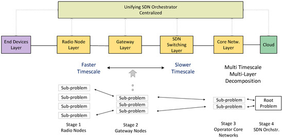
Figure 1.
Illustration of LayBack architecture and multi-timescale optimization decomposition in context of cellular networks: LayBack partitions the wireless backhaul infrastructure into radio node layer, gateway layer, SDN switching layer, and core network layer. The entire network is controlled by the central unifying SDN orchestrator. This case study decomposes the optimization of the sharing of the backhaul bitrate of multiple operator core networks into fast-timescale sub-problems at the radio nodes and progressively slower timescale sub-problems at the gateways and operator core networks; whereby all sub-problems are coordinated through a root problem at the SDN orchestrator.
3.2. Management in LayBack
The unifying SDN orchestrator in LayBack has three main tasks: (1) it creates a common platform for coordinating among all the wireless service operators and heterogeneous network technologies across its layers; (2) it maintains the current topology information of the entire network and tracks the network capabilities; (3) it enables each of the layers to flexibly reconfigure the network by allocating resources in response to their time-varying needs, while maintaining long-term performance requirements that define the service guarantees. The networks maintained by different operators periodically communicate their requirements and reconfiguration capabilities to the SDN orchestrator to enable the SDN orchestrator to fulfill its tasks. Next, we show how these tasks can be combined with an online optimal resource sharing task that leverages our multi-layer multi-timescale NUM framework.
4. Layered SDN-Based Optimization Framework
4.1. Overview
This section formulates a multi-layer multi-timescale optimization model for the backhaul resource sharing in LayBack. The optimization model is decomposed into multiple layers so that the orchestrator centrally controls the resource sharing among the operators, while distributing the decision-making processes to ensure scalability. The multiple timescales facilitate quick dynamic reactions to the needs of the network end users while accommodating the signaling delays to the central SDN orchestrator.
In our optimization model, we abstract away the actual relationships between the physical layer wireless communication resources (i.e., spectrum and power) at the radio node layer (eNB, Wi-Fi AP) and the corresponding dynamic allocation of the bitrate. We focus on the management of an abstract total backhaul bitrate resource Z, which is indirectly tied to the redistribution of the physical layer wireless communication resources. The SDN-based LayBack architecture maintains a logically separated queue at each radio node. The shared resource Z trickles down from the unifying SDN orchestrator to the operators, from each operator to its gateways (GWs) and, finally, from each GW to its radio nodes.
4.2. Model Definitions
We consider a network with O distinct operators, indexed by . (The main model definitions are summarized in Table 1.) Each operator manages a set of GWs indexed by . In turn, each GW g manages a set of eNBs, indexed by . Let us also define the set of all the eNBs and the set of all the GWs. The queue at a given eNB is denoted by and its dynamics are
where and represent, respectively, the exogenous packet arrival process and the backhaul service rate that is granted to eNB n during time slot t. Also, denotes the projection onto the nonnegative orthant (). The service rate represents the backhaul (bitrate) resources allocated for the upstream (eNB to GW) transmission between t and to the specific eNB n.

Table 1.
Summary of model notations.
The multi-layer multi-timescale optimization framework developed in this section is applicable for the wide range of optimal resource allocations to distributed entities. In particular, the developed optimization framework is well suited for scenarios with substantial signaling delays between the distributed entities and a central controller so that purely centralized decisions are impractical. Aside from large-scale wireless access networks, such resource allocation problems arise for instance in supply and demand management [83] and in transactive energy markets [84,85,86,87].
4.3. Centralized Queue Length Minimization
Before introducing our timescale decomposition, we start from the centralized optimization we wish to emulate, and the logical steps that decompose the problem into layers via the Lagrange decomposition. If the SDN orchestrator, with full control of the total service rate Z, could allocate rates directly to the eNBs, the optimization would be:
where we use the QMW policy as objective function with for the sake of illustrating the decomposition technique. In this formulation, the first constraint represents the overall backhaul capacity, whereas the second constraint defines the feasible region for optimization variable which is limited by serving all packets in the queue per one time slot. We remark that an alternative optimization case study would be to consider the wireless device queues as the bottom layer queues. For such an alternate optimization model with wireless device queues, the utility should include the state w of the wireless channel which could be incorporated as , whereby f is a known function of the queue, channel state information w, and service rate .
With the QMW policy, the maximization in (2) leads to the minimization of the long-term average total queue length, which also results in the minimization of the end-to-end delay in the network (a consequence of Little’s theorem [88] for the simplified scenario of continuous flows and infinite queue backlogs [89]).
4.4. Operator Resource Constraints
There are two potential problems with solving (2): (1) the allocation of network resources at the level of granularity of individual eNBs may result in scalability problems; and (2) without any long-term constraints, some operators may hoard backhaul resources. In order to create multiple layers to distribute the decision-making processes, we rewrite the maximization in (2) by introducing variables that for the sake of solving (2), are slack variables. As we will see, the additional variables represent actual network decisions in the distributed and time-decomposed implementation of the centralized scheduler.
In particular, let us denote by the portion of the wireless service rate Z that is distributed to operator o and let denote the vector of allocated operator service rates. Each operator , redistributes the resources, by giving a portion of to each of its GWs , whereby we denote for the vector of GW rate allocations of operator o. In turn, each GW g redistributes the resources, by giving a portion of to each of its eNBs , whereby we denote . If all these assignments could happen at the same timescale indexed by t, distributing the constraints at each layer, the optimization could be solved as follows:
with being the optimal value of the subproblem:
and being the optimal value of
It is important, however, to remark that the allocation of to solve (3) needs to respect an “economic” constraint across the operators that defines a contractual service obligation and prevents any operator from gaming the system (i.e., consistently acquiring more resources than what it paid for). This constraint on the long-run average of the decisions is:
where for consistency of the problem, it is necessary to have . At the same time, by having an inequality constraint, we are not forced to assign resources to an operator that would be wasted if there is not sufficient uplink demand.
We use the concept of virtual queues, following the Lyapunov drift-plus-penalty approach [51] to encode the constraint in (6), and we modify the objective in (3) into:
After deciding , the virtual queues are updated as:
where is the fixed average maximum resource limitation of operator o.
The parameter V represents the “flexibility” of the constraint in (6), e.g., the higher V the more inclined we are to temporarily violate the constraint. The next subsection serves as a basis to tackle the problem at different timescales that are aligned with the network infrastructure, as elaborated in Section 4.6. It is however easier to derive them in the ideal static case first, given that the expressions in the dynamic case will have the same form, albeit with different meanings.
4.5. Iterative Solution via Gradient Descent
We omit the time index t to avoid notational clutter. The dual objective function of the subproblem (3) can be written as
whereby denotes the vector of queue occupancies. We introduce the Lagrangian dual variable for the constraint in (3), the Lagrangian dual variables for the constraints in (4), and the Lagrangian dual variables for the constraints in (5). Then, unfolding all the constraints, we obtain (10) and following a cascade of primal dual decompositions (see [42]), the optimization can be solved via the sequence of projected gradient descent updates:
where the different denote step sizes. The bottom layer optimization in (9) can be solved with Algorithm 1, while the solution for a general utility is shown in [90]. We note that to ensure the convergence of the decomposition, the updates in (11)–(14) must be read as follows: to reach the optimal , the SDN orchestrator needs to perform a sufficient number of iterations in (11). However, before computing one iteration of (11), the operator layer below should perform a sufficient number of iterations of (12) upon receiving the Lagrangian , and so on. Unless a value can be computed in closed form in one shot, each update that includes the solution of an optimization problem (i.e., it has an argmax or argmin term in the update) requires a sufficient number of gradient descent updates at the lower level to approximate the solution of the subproblem. Therefore, the indices k in (11)–(14) are not associated with the same timescale. If the computation at each layer and the communication delays among layers were all negligible, we would be in the timescale separation regime [42,43]. However, this is not possible in a real system, since latencies play a significant role in real networks and the framework we are about to explain explicitly takes these latencies into consideration. We also note that in this decomposition model, there is no sharing of information among the operators, which makes the model more practical. All message passing occurs only between neighboring layers, whereby the lower layer sends the optimal resource allocation and the upper layer sends the dual variable.
| Algorithm 1: Solution of (9) (at GW g). |
 |
Let us start by considering the optimization at the bottom layer as the one that operates at the minimum latency, i.e., the time difference between the time indexes t and is the Round Trip Time (RTT) between GW and eNB (considered equal, for simplicity, for all GWs and eNBs), since it is the one closest to the devices and to the information regarding traffic. To map all the time instants into integer values of t, it is convenient to normalize all times with respect to (i.e., we set ).
Our framework considers that in actual network infrastructures one has constraints that prevent the redistribution of the total resource across the operators (e.g., the decisions ) and redistribution of operator resources across the GWs (e.g., the decisions ) from changing at the same timescale of the redistribution of GW resources across the eNBs (e.g., the decisions ). Therefore, even if a genie could compute the optimal solution of the decomposed problem at each instant t, it might not be possible to implement the decision.
Denoting with and the minimum refresh times for the GW decisions and for the operator’s decisions , respectively, time t can be written according to a poly-phase decomposition as
where and are the selected refresh times. We illustrate the multi-timescale dynamics of the optimization framework in Figure 2 showing the interactions of eNBs, GWs, operators, and SDN orchestrator.
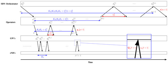
Figure 2.
Illustration of the dynamics of the multi-timescale optimization framework within context of LayBack infrastructure: the optimal policy to minimize end-to-end delay is decoupled into multiple layers of sub-problems, with faster timescales at the lower LayBack layers The eNBs , at a GW g pass their queue occupancies each eNB-GW round-trip time RTT to GW g. Based on the received vector of queue occupancies , GW g evaluates the allocations to its eNBs with Algorithm 1. Similarly, the SDN orchestrator evaluates the allocations to the operators with Algorithms 2 and 3; while each operator o evaluates the allocations to its GWs with Algorithms 4 and 5. (In order to reduce clutter, the eNB-to-GW RTT has been normalized to one in the illustration, i.e., in the illustration corresponds to in actual time).
In the next subsection, to comply with the refresh time limits, the greedy optimization, decoupled at any instant t, is mapped into the stochastic optimization we solve. Changing the objectives from deterministic values to expected values is necessary to capture the uncertainty of the impact of the decisions and on the future queues evolving at a faster timescale, e.g., on the effect that a change in higher layers’ resources distribution, produces on the lower layers’ optimizations.
| Algorithm 2: At the SDN orchestrator. |
 |
| Algorithm 3: Iterates for (at operator o). |
 |
| Algorithm 4: Iterates for (at operator o). |
 |
| Algorithm 5: Iterates for (at GW g). |
 |
4.6. Stochastic Optimization and Temporal Decomposition
Since the different layers cannot communicate instantaneously, the parameters of the queues change dynamically underneath. Clearly, the objectives of the optimization must be defined in such a way that they stay constant while the bottom layer changes stochastically from one state to the next. The proposed framework can be seen as a special case of stochastic gradient descent where the network dynamics, via the evolution of the queues, impose the sequence of training sample updates. In particular, the SDN orchestrator operates its optimization at every time instant , performing
with equal to the optimal value of the problem solved at the operator layer below:
and being the optimal values of the optimization in (5) for . The updates derived in (11)–(14) will then be used to update the decisions every and the decisions every L, as if convergence to the solution of a static problem has been achieved in the time horizons of length and L, respectively. By introducing as the number of iterations of each update in layer respectively, starting from the bottom, we can derive the following relations:
where , , and , are, respectively, the RTTs between the SDN orchestrator and the operators, between the operators and the GWs, as well as between the eNBs and the GWs (see also Figure 2, where has been normalized to one). The inequalities in (18)–(19) indicate that if we want to act fast, e.g., reduce P and L (possibly to the minimum refresh times) we need to perform fewer iterations. Vice versa, if we want to perform more iterations, we must be willing to act slower in updating the decisions and . If we view the static problem as a “surrogate” for the dynamic problem (up to the next decision), increasing the number of iterations and delaying future decisions can guarantee a better accuracy for a static scenario; however, the ability of the algorithm to incorporate new dynamic information is compromised. This trade-off creates another optimization issue which is an important future research direction.
5. Numerical Evaluation Results
In this section, we describe the evaluation setup for this numerical optimization case study and discuss the evaluation results obtained with the optimization approach described in the preceding section.
5.1. Evaluation Setup
We have implemented the optimization framework described in Section 4 in MATLAB to evaluate the allocation of the backhaul bitrate resources in the upstream path in LayBack. The upstream data path consists of eNB, GW, and an operator core network.
5.1.1. LayBack Architecture
Initially, we consider a LayBack network architecture with network operators, which we index with and . Each network operator has three GWs for a total of six GWs. Each gateway has ten eNBs for a total of 60 eNBs.
Each operator has an installed backhaul bitrate resource (capacity) of Mbps. Assuming that the two operators have agreements to fully share each other’s backhaul capacity, the aggregate available backhaul bitrate (capacity) is Mbps. The objective of the optimization is to optimally share the available backhaul resource of Mbps among all eNBs attached to all the GWs of both operators and .
The round-trip propagation delays (RTTs) are set to eNB-GW RTT ms, GW-operator RTT ms, and operator-SDN orchestrator RTT s.
5.1.2. Optimization Parameters
The iteration parameters are set to , , , and . Following the lower bounds imposed by the K values in Equations (18) and (19), we set and . By default, we set the mean drift-plus-penalty parameter to . For all the updates, and for numerical stability, the computation of considers the queue normalization , which does not alter the solution.
5.1.3. Comparison Benchmark
The baseline in our evaluation is the performance of a no-SDN wireless scheduling framework, i.e., the absence of the LayBack orchestrator to coordinate the scheduling. As a result, each operator o can only occupy its own backhaul bandwidth , i.e., there is no inter-operator bandwidth sharing. More specifically, in our simulations, the no-SDN benchmark solves only the optimization up to the subproblem Equation (4) with the dynamic operator allocation replaced by the static operator capacity , and the subproblem Equation (5) [but not the subproblem Equation (3)]. That is, the no-SDN benchmark only optimizes the allocations within each given operator individually, i.e., performs essentially only “intra-operator” optimization. The no-SDN benchmark follows the same multi-timescale behavior with , , and as the SDN-based optimization. We report the aggregate of the gateway allocations for operators and 2 as the actual allocated operator upstream bitrates of the no-SDN benchmark; whereas, for the SDN-based optimization, we report the operator rate allocations .
We note that an alternate benchmark without any optimization could consider a static allocation of backhaul capacity portions to individual eNBs. Such a static allocation would perform poorly for dynamic bursty traffic models, as specified in Section 5.1.4. The static allocation would incur substantially longer queue lengths than the considered “intra-operator” optimization, which individually independently optimizes the allocations within each operator. Another alternative benchmark could employ conventional two-layer NUM between the eNBs and the operators (with the gateways subsumed by the operators). Such a two-layer benchmark would still perform the intra-operator optimization, but with only two layers compared to the three layers in the considered benchmark. These two benchmarks would generally perform similarly, with differences being influenced by convergence characteristics [79]. For the present study, we focus on the impact of the sharing of the backhaul resource across operators as quantified by comparing the considered no-SDN “intra-operator” optimization with the full SDN-based optimization involving the central SDN orchestrator.
5.1.4. Traffic Model
We model the upstream packet traffic generation at a given eNB (which is due to upstream packet arrivals from associated user end devices [91]) as an independent Poisson process. We set the eNB Poisson process rates such that the aggregate load from the eNBs at a given operator o results in a base packet traffic load of 5 Mbps, whereby each of the 30 eNBs at a given operator o contributes equally to the aggregate operator load. We conduct simulations of 100 s of backhaul network operation, whereby the Poisson traffic generation occurs over time increments of 0.1 ms, i.e., one simulation run of 100 s corresponds to one Million Poisson packet traffic generation instantiations.
We consider dynamic upstream traffic variations, which can, for instance, be caused by new temporary connection establishment or data connection handovers, e.g., due to user mobility. Specifically, we initially simulate a peak load of 20 Mbps occurring by default at operator 1 from 10 to 20 s of a simulation run and at operator 2 from 50 to 60 s of a simulation run.
5.2. Results
5.2.1. Temporal Spacing of Operator Peak Demands
Overlapping Peak Demands
We first verify the correct operation of the SDN-based optimization for a scenario that does not permit inter-operator bitrate sharing, specifically, for a scenario where the peak periods of the upstream bitrate demand at the eNBs of the two operators occur simultaneously, as illustrated in Figure 3a. Both operators experience a jump of the demanded upstream bitrate from 5 Mbps to 20 Mbps at simulation time 10 s; the 20 Mbps peak load persists for 10 s, and then returns to the 5 Mbps base load level. Note that these load levels correspond to the prescribed Poisson process rates, i.e., the actual load levels vary according to the stochastic characteristics of the Poisson packet generation processes around the prescribed bitrates, as is visible through the slight random “ripples” of the demand bitrates in Figure 3a.
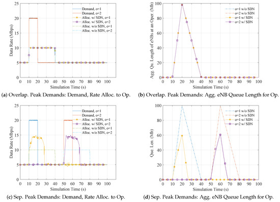
Figure 3.
Upstream traffic demands and corresponding backhaul bitrate allocations to operators as well as aggregated queue length of eNBs associated with a given operator when peak demand periods of the two operators overlap or are separated (fixed parameter: Mean drift-plus-penalty parameter ): For overlapping peak demands (a,b), both the SDN-based optimization and the benchmark without SDN allocate to each operator its maximum capacity of Mbps to serve the peak demands; there is no sharing among operators. For separated peak demands (c,d), the SDN orchestrator dynamically shares the total aggregated backhaul capacity of Mbps among the two operators, reducing eNB queue lengths compared to the benchmark without SDN-based resource sharing.
We observe from the curves for the allocated operator rates ( with SDN, without SDN) in Figure 3a that both the SDN and no-SDN approaches allocate the maximum operator rate of Mbps to serve the peak load. Since both operators experience the peak load at the same time, sharing among operators would not be sensible. Rather, each operator o should use its own full upstream bitrate resource to minimize packet delays. We observe from Figure 3a that the SDN-based optimization meets this intuitive optimization goal and gives essentially the same rate allocations as the no-SDN benchmark. In particular, given the equal demands from the eNBs of both operators, the SDN-based optimization strives to allocate an equal share of half of the total upstream backhaul bitrate of Mbps to each operator while serving the peak load. Thus, for the entire simulation time duration, the resource allocation with SDN-based optimization follows the resource allocation without SDN.
The no-SDN benchmark solves the optimization up to the subproblem Equation (4), whereby the operator upstream transmission capacity is limited to Mbps with the considered parameter settings. Thus, by solving subproblem (4), each operator in the no-SDN benchmark is able to allocate up to Mbps when a demand burst occurs.
We note that a conventional static allocation of backhaul bitrate (without any dynamic optimization, not even the intra-operator optimization of the no-SDN benchmark) would allocate Mbps for the entire simulation duration. However, only 5 Mbps out of these 10 Mbps could be used during the time period from 0 to 5 s and from 40 s onwards to the end of the simulation time, thus leading to wasted backhaul bandwidth.
We observe from Figure 3b that the queue lengths of the eNBs at both operators linearly increase at a constant rate since both operators experience the same peak load that exceeds their respective available backhaul bitrate . In particular, the queue lengths increase from 0 to a maximum value corresponding to 10 s Mbps = 100 Mbit while the peak load is feeding into the eNBs from 10 to 20 s simulation time. Subsequently, the queue length decreases down to zero over 20 s as effectively an “extra” backhaul bitrate of 5 Mbps, i.e., the allocated 10 Mbps minus the currently served base load of 5 Mbps, is serving the backlog from 20 s to 40 s simulation time.
Separated Peak Demands
Figure 3c,d considers the more typical operational scenario when peak demands for the different operators are separated in time, e.g., due to different traffic and mobility patterns of the end users. We observe from Figure 3c that the SDN-based optimization with backhaul resource sharing among the two operators allocates up to 15 Mbps to the operator that currently experiences the peak demand (while 5 Mbps continue to serve the other operator); thus fully using the total available backhaul bitrate Mbps. In contrast, the benchmark without SDN does not share backhaul capacity among operators. Accordingly, without SDN, operator 1 can only serve the peak demand that occurs from 10–20 s with its own 10 Mbps capacity; meanwhile, operator 2 uses only 5 Mbps of its 10 Mbps capacity and the other 5 Mbps are wasted.
The SDN-based backhaul resource sharing reduces the queue build-up in the eNBs, as observed in Figure 3d compared to the benchmark without SDN, implying shorter latencies with SDN-based sharing. The slight variations between the optimization behaviors for the peak demands of operators 1 and 2 are due to the random variations of the actual demands around the prescribed mean Poisson traffic rates.
5.2.2. Impact of Flexibility Parameter V
The mean-plus drift parameter V in the optimization framework, see Equation (7), relates to the degree of flexibility with which the operators can share the total aggregate backhaul capacity Z beyond their own backhaul capacity . Figure 4 shows the performance of the resource allocation algorithm for increasing values of the flexibility parameter V, namely for , 10, and 100, while for we refer to Figure 3c,d. Moreover, Figure 4g,h shows the optimization performance without the economic constraint (6). We observe from Figure 4a,c that for small V values, e.g., and 10, the rate allocation with SDN optimization is nearly equivalent to the no-SDN benchmark. The small differences between the allocations with the SDN optimization and the no-SDN benchmark are mainly some low-amplitude oscillations in the SDN allocations. The allocation oscillations result from the optimization framework striving to adapt to slight random variations in the traffic generation processes. Accordingly, both the SDN optimization and the no-SDN benchmark give essentially the same eNB queue lengths as observed from Figure 4b,d. Intuitively, small V values restrict the drift from the mean in the optimization framework, which inherently corresponds to a low degree of flexibility when operators want to share each other’s resources.
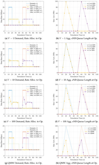
Figure 4.
Upstream backhaul bitrate allocations and eNB queue lengths when demand peaks for operators 1 and 2 are spaced apart: Increasing the “flexibility parameter” V, see Equation (7), increases the sharing of backhaul capacity among the two operators and decreases the queue lengths compared to the benchmark without SDN orchestrated backhaul resource sharing; for , please refer to Figure 3c,d. The QMW case corresponds to the SDN-based optimization without a long-term constraint.
In contrast, we observe for the higher and 1000 values in Figure 4f and Figure 3d that SDN optimization with flexible backhaul resource sharing among operators achieves smaller eNB queue lengths than the no-SDN benchmark. We observe that the queue lengths for in Figure 3d are nearly as small as the queue lengths in Figure 4h for optimization without the long-run rate allocation constraint. Indeed, the rate allocation without the rate allocation constraint in Figure 4g is being approximated by the SDN rate allocation in Figure 3c. The rate allocation constraint safeguards against persistent unfair backhaul capacity usage by a given operator and is therefore generally recommended for operational networks.
5.2.3. Impact of Spacing between Operator Traffic Bursts
While Figure 3 and Figure 4 considered a fixed 40 s separation of the starting time instants of the data bursts (of 10 s duration) at the two operators, we consider a range of burst separations in Figure 5. We observe from Figure 5 that a burst separation of zero, which corresponds to the scenario in Figure 3a,b does not permit queue reductions through backhaul resource sharing. In contrast, the 40 s separation of the data bursts corresponding to the scenario in Figure 3c,d as well as Figure 4, does permit the sharing of the backhaul resources of the two operators. Thus, with the large flexibility parameter setting, substantial reductions of the average eNB queue lengths can be achieved for both operators for large separations of the data bursts.
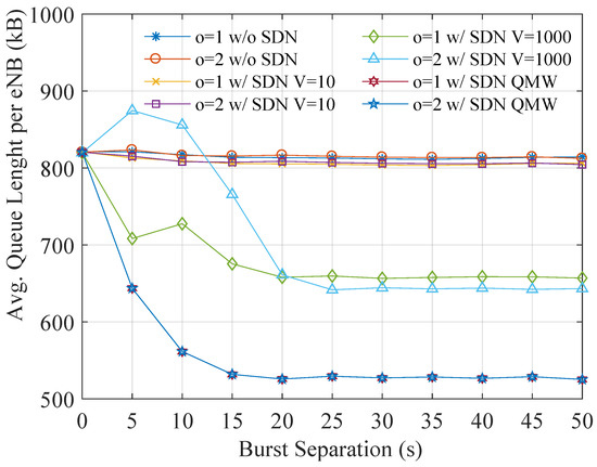
In contrast, for the short separation times of 5 s and 10 s, we observe from Figure 5 that operator achieves queue length reductions for the large setting, whereas the queue lengths for operator increase. The eNBs at operator , which receives the earlier data burst, can still achieve queue length reductions by using some of the backhaul capacity of operator to serve the data burst arriving to the eNBs at operator . However, the use of the capacity by the burst when the data burst to the eNBs at operator arrives, slows down the service for the burst, resulting in the queue length increases observed in Figure 5. However, we observe from Figure 5 that the average of the curves for and for the setting is slightly below the corresponding queue length averages for operation without SDN or with the inflexible . Thus, the flexible sharing of backhaul capacity with does not “harm” the overall system compared to operation without sharing. The QMW benchmark gives yet lower queue length as QMW shares the bandwidths of the two operators without any constraints, i.e., corresponds to V approaching infinity (which would not enforce fair bandwidth allocations to operators).
5.2.4. Impact of Random Traffic Bursts at Operators
The traffic model from Section 5.1.4 consisted of eNB Poisson packet traffic, whereby the eNB Poisson traffic rates at a given operator o were set to result in traffic bursts at prescribed times, as examined in Section 5.2.1 through Section 5.2.3. We now generalize this traffic model to random traffic bursts as follows. The eNBs continue to generate independent Poisson packet traffic. The eNB Poisson packet rates at a given operator , follow an independent two-state (on and off) Markov chain. In the on state, the 30 eNBs at a given operator generate an aggregate Poisson traffic rate of 20 Mbps; while in the off state, there is no packet generation. Both states have exponentially distributed random sojourn times with a mean of 10 s. The load is varied by adjusting the steady-state probability of being in the on state and each simulation scenario is run for 1000 s.
Figure 6a shows the mean eNB queue length as a function of the on-state probability , i.e., effectively as a function of the load level. We observe from Figure 6 that the SDN control achieves eNB queue length reductions across the entire stable load range from a small on-state (burst) probability up to a load level near the stability limit, which would be reached for . The eNB queue length reduction appears initially modest for small because the bursts are rare for low , i.e., the behavior is similar to the individual burst scenario considered in Figure 3 and Figure 4 and thus can be cleared relatively quickly, even without SDN control. For increasing , the bursts become more frequent, the eNB queue backlogs increase and flexible SDN control with achieves substantial queue reductions compared to operation without SDN control and compared to a less flexible SDN control with .
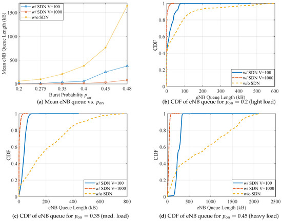
Figure 6.
Mean and CDF of eNB queue length in kB for operators with random traffic burst as a function of steady-state probability of burst state.
Figure 6b–d show the cumulative distribution function (CDF) of the eNB queue occupancy for three load levels, represented by different . We observe from Figure 6b–d that the CDF curves for SDN control reach the level of one within a much smaller span of eNB queue lengths than the operation without SDN control. For instance, for the medium load level , the CDF for the SDN control with reaches one for a queue length of about 90 kB; whereas, operation without SDN control reaches a CDF level of one only for around 760 kB eNB queue length. Thus, the CDF results indicate vastly reduced variability of the eNB queue length with the SDN control as the SDN control reacts to the traffic bursts by actively re-allocating backhaul resources among the considered operators.
We observe from Figure 6d that for the low eNB queue occupancies in the range up to about 200 kB, operation without SDN control achieves higher probabilities of keeping the eNB queue lengths in this low range than SDN control with . This is mainly because the SDN control strives for fairness. If some eNB has a small queue occupancy compared to the other eNBs, the SDN control balances out the eNB queue occupancies via the centrally coordinated backhaul bandwidth allocation. In particular, the CDF curve for SDN control with indicates that almost all the queue occupancies occur around the 200 to 250 kB range (the larger allows for flexible violations of the fairness constraint while sharing the backhaul bandwidth and thus achieves substantially lower queue occupancies). If some services do not want to be subjected to this fairness guided resource allocation and rather want priority service, then the priorities can be implemented through weights for their utilities.
We considered only operators sharing the overall backhaul resource Z in this section. When a larger number O of operators shares the overall resource, then the performance of the SDN control would further improve in accordance with the classical statistical multiplexing gains for many variable bitrate traffic streams sharing a common resource [28,61,92,93,94]. In this and the preceding evaluation scenarios, traffic bursts were generated on a per-operator basis, i.e., an independent Markov chain for each operator , determined the Poisson packet traffic rates (whereby the eNBs at an operator contributed equally to the operator traffic load). This per-operator traffic burst scenario reflects situations where traffic demands shift among operators, e.g., as large groups of users move among different nearby sub-networks, e.g., from lecture halls to restaurants (whereby the lecture halls and the restaurants have different operators) in a campus setting. In the next section, we consider per-eNB Markov chain modulated Poisson packet traffic rates that reflect situations where each eNB generates traffic bursts independently, e.g., when individual users conduct bursty Internet transactions, e.g., upload files.
5.2.5. Impact of Random eNB Traffic Bursts
To evaluate the multi-layer multi-timescale approach for a large-scale network with independent eNB traffic bursts we modify the LayBack architecture from Section 5.1.1 as follows. We consider operators, each with two GWs; each GW has five eNBs, for a total of 200 eNBs. The overall backhaul capacity still equals Mbps, but the operator backhaul capacity is Mbps. We consider this large network for random eNB Poisson packet traffic bursts generated according to an independent two-state (on and off) Markov chain for each of the 200 eNBs. An eNB generates 0.2 Mbps of Poisson packet traffic in the on state (fixed sojourn time of 10 s) and no traffic in the off state (exponentially distributed random sojourn time with mean 20 s for low load, 15 s for medium load, and 12 s for high load). The stationary distribution of visits to the on and off states is kept at 0.5 and 0.5. The resulting long-run traffic load for the medium load scenario is 16 Mbps (=200·0.2 Mbps·(0.5·10 s)/(0.5·10 s + 0.5·15 s)), while the long-run traffic loads for the low and high load scenarios are 13.3 Mbps and 18.2 Mbps, respectively.
We observe from Figure 7a that for the light load scenario the SDN orchestrated backhaul bitrate allocation increases the probabilities for low eNB queue occupancies below 50 kB only relatively slightly compared to the operation without SDN. In contrast, we observe from Figure 7b vastly increased probabilities for low eNB queue occupancies below 50 kB with the SDN control compared to operation without SDN. More specifically, SDN control keeps the eNB queue lengths below 50 kB with a probability near one, whereas queue lengths below 50 kB occur only with a probability of about 0.4 without SDN control.
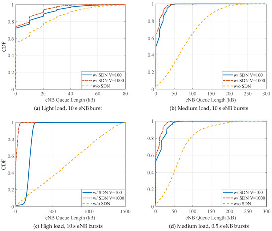
Figure 7.
Cumulative distribution function (CDF) of eNB queue length for independent eNB traffic bursts with various load levels for long (10 s) bursts and medium load for short (0.5 s) bursts; fixed parameters: operators, each with two gateways (each with five eNBs).
If five or fewer eNBs at a given operator are in the on (traffic burst of 0.2 Mbps) state, then the aggregate traffic of the ten eNBs at the operator can be accommodated within the operator backhaul capacity of Mbps. If six or more eNBs at a given operator are in the traffic burst state and another operator has less than five eNBs in the traffic burst state, then the SDN control can share the backhaul resource among the operators. For the light traffic scenario (Figure 7a), occurrences of six or more simultaneous eNB traffic bursts at a given operator occur only occasionally; thus, there are relatively few opportunities for SDN control to share backhaul resources.
For the medium and high load levels (Figure 7b,c) it becomes increasingly likely that the aggregate load from the ten eNBs at a given operator exceeds the operator backhaul capacity . At the same time, due to the general Poisson process clumping behaviors [95,96], it is likely that the eNB traffic bursts “clump” at a given operator and exceed , while other operators have spare backhaul capacity. Thus, central SDN control of the backhaul capacity allocation can achieve substantial eNB queue length reductions compared to the operation without SDN.
Regarding the flexibility parameter V, we observe from Figure 7 that the benefit of the large relative to the smaller increases as the load increases from the light/medium load to the high load. This is mainly because, is essentially the penalty for using spare bandwidth from other operators. For the light and moderate load levels, there are only relatively rare to moderately frequent occasions of bandwidth sharing; thus, there is no pronounced effect of V. For the high load (which corresponds to a long-run average overall backhaul use of 10/12), the assumption of the Lyapunov optimization is satisfied (i.e., the queues are stable), allowing the increased V to reduce the queue lengths.
Figure 7d considers the medium load scenario for short eNB bursts of 0.5 s (with corresponding 0.75 s off state sojourn time). Comparing Figure 7b,d, we observe that the operation without SDN achieves shorter eNB queue lengths with the short bursts in Figure 7d compared to the long bursts in Figure 7b. For example, an eNB queue length under 100 kB is achieved with over 0.8 probability in Figure 7d, but only less than 0.65 probability in Figure 7b. Intuitively, the shorter eNB traffic bursts create only smaller eNBs queue backlogs that are easier to clear with the limited operator bandwidth . We also observe from the comparison of Figure 7b,d that the gap between SDN control with and with has slightly widened in Figure 7d, mainly due to the CDF curve for reaching only lower values in Figure 7d compared to Figure 7b. This is primarily because the shorter burst in Figure 7d require more flexibility from the SDN control; however, the control provides only limited flexibility and can therefore not perform quite as well as for the longer bursts in Figure 7b. Nevertheless, even though the gap between operation with SDN control vs. operation without SDN control has slightly shrunken in Figure 7d compared to Figure 7b, the SDN control still achieved substantial eNB queue length reductions.
6. Conclusions
This article has presented a multi-timescale approach for optimizing the sharing of backhaul resources in the SDN-based layered backhaul (LayBack) network architecture. Through primal dual decomposition and Lyapunov drift techniques we decomposed the traditionally centralized SDN resource management into a distributed management model. The distributed resource management accommodates realistic signaling propagation delays by conducting optimization computations at the higher gateway and SDN orchestrator layers at slower timescales compared to the fast-timescale operation at the eNB radio nodes. The distributed optimization is also highly scalable as only slow timescale optimizations of the sharing of the backhaul resources among multiple operators are performed at the central SDN orchestrator; the finer-grained faster timescale resource allocations to the individual eNB radio nodes and various gateway nodes are performed at the lower layers of the multi-layered multi-timescale optimization.
Our numerical evaluations for backhaul example networks have quantified the performance characteristics of the described multi-timescale backhaul resource optimization. We found that the SDN controlled sharing of the backhaul resources among operators can significantly reduce the queue lengths at the radio nodes, e.g., the eNBs that serve the upstream traffic from the wireless end users, compared to an optimization without SDN controlled resource sharing.
There are many interesting directions for future research on optimizing the backhaul in wireless networks. This present case study has focused on demonstrating the feasibility of a multi-timescale optimization with a specific example optimization methodology (gradient descent combined with Lyapunov drift-plus-penalty method) in a specific configuration of the LayBack backhaul network architecture. Future research should examine how wireless backhaul network architectures should be dimensioned, e.g., how many layers and how many nodes should be in a given layer for a range of anticipated end-device densities and mobility patterns over the geographic area covered by the wireless backhaul network architecture, so as to best support the optimization processes for resource allocation. With the emergence of multi-access edge computing (MEC) it may become important to widen the scope of resource allocation optimization to cover communication, caching (storage), and computation (e.g., virtual machine compute processing) resources [97,98,99]. Moreover, the suitability of the various types of optimization methodologies for the resource allocation in wireless backhaul networks should be broadly studied and compared. The comparison should consider both the optimization performance as well as the practical operational aspects, e.g., simplicity and computation resource usage. Another important future research aspect is robustness and reliability of the wireless backhaul network. Emerging cyber-physical systems, such as medical devices that provide critical diagnostics and continuous therapeutic interventions to humans going about their daily lives [100] as well as networked vehicular systems [101,102,103], such as the transportation systems in smart cities, require uninterrupted connectivity with high quality of service levels. Wireless backhaul networks need multiple redundant connectivity paths that provide fail-over functionalities in case of failures [104,105,106]. Future backhaul resource optimization needs to account for and route among these multiple connectivity paths (e.g., with SDN support [107,108]) and optimally allocate resources during normal operation as well as after various failure scenarios. Furthermore, it would be of interest to implement the SDN controlled backhaul resource sharing in SDN testbeds [109,110,111] to verify the resource sharing performance characteristics in real operational networks.
Author Contributions
Conceptualization, A.S., L.F., M.R. and A.S.; Methodology, M.W., N.K., L.F., P.S., A.S.T., M.R., and A.S.; Software, M.W., N.K., L.F., and P.S.; Validation, N.K., L.F., and A.S.T.; Formal Analysis, N.K., L.F., and A.S.; Investigation, M.W., L.F., and M.R.; Resources, M.R. and A.S.; Data Curation, M.W., N.K., and P.S.; Writing—Original Draft Preparation, L.F., A.S.T., M.R., and A.S.; Writing—Review and Editing, M.R. and A.S.; Visualization, M.W., L.F., and A.S.T.; Supervision, M.R., and A.S.; Project Administration, A.S.T., M.R., and A.S.; Funding Acquisition, M.R., and A.S.
Funding
This research was funded by the U.S. National Science Foundation grant number 1716121.
Conflicts of Interest
The authors declare no conflict of interest. The funders had no role in the design of the study; in the collection, analyses, or interpretation of data; in the writing of the manuscript, or in the decision to publish the results.
References
- Ferrari, L.; Karakoc, N.; Scaglione, A.; Reisslein, M.; Thyagaturu, A. Layered Cooperative Resource Sharing at a Wireless SDN Backhaul. In Proceedings of the IEEE International Conference on Communications Workshops (ICC Workshops), International Workshop on 5G Architecture (5GARCH), Kansas City, MO, USA, 20–24 May 2018; pp. 1–6. [Google Scholar]
- Andrews, J.; Singh, S.; Ye, Q.; Lin, X.; Dhillon, H. An overview of load balancing in HetNets: Old myths and open problems. IEEE Wirel. Commun. 2014, 21, 18–25. [Google Scholar] [CrossRef]
- Lopez Rodriguez, F.; Silva Dias, U.; Campelo, D.R.; Oliveira Albuquerque, R.D.; Lim, S.J.; Garcia Villalba, L.J. QoS Management and Flexible Traffic Detection Architecture for 5G Mobile Networks. Sensors 2019, 19, 1335. [Google Scholar] [CrossRef] [PubMed]
- Hassan, T.U.; Gao, F. An Active Power Control Technique for Downlink Interference Management in a Two-Tier Macro–Femto Network. Sensors 2019, 19, 2015. [Google Scholar] [CrossRef] [PubMed]
- Mikaeil, A.M.; Hu, W.; Hussain, S.B.; Sultan, A. Traffic-Estimation-Based Low-Latency XGS-PON Mobile Front-Haul for Small-Cell C-RAN Based on an Adaptive Learning Neural Network. Appl. Sci. 2018, 8, 1097. [Google Scholar] [CrossRef]
- Wang, N.; Hossain, E.; Bhargava, V. Backhauling 5G small cells: A radio resource management perspective. IEEE Wirel. Commun. 2015, 22, 41–49. [Google Scholar] [CrossRef]
- Yang, W. Conceptual Verification of Integrated Heterogeneous Network Based on 5G Millimeter Wave Use in Gymnasium. Symmetry 2019, 11, 376. [Google Scholar] [CrossRef]
- Kelly, F.P.; Maulloo, A.K.; Tan, D.K.H. Rate Control for Communication Networks: Shadow Prices, Proportional Fairness and Stability. J. Oper. Res. Soc. 1998, 49, 237–252. [Google Scholar] [CrossRef]
- Lin, X.; Shroff, N.B.; Srikant, R. A tutorial on cross-layer optimization in wireless networks. IEEE J. Sel. Area Comm. 2006, 24, 1452–1463. [Google Scholar]
- Chiang, M.; Low, S.H.; Calderbank, R.; Doyle, J.C. Layering as optimization decomposition. Proc. IEEE 2007, 95, 255–312. [Google Scholar] [CrossRef]
- Chiang, M. Stochastic network utility maximization. Eur. Trans. Telecommun. 2008, 22, 1–22. [Google Scholar]
- Shantharama, P.; Thyagaturu, A.S.; Karakoc, N.; Ferrari, L.; Reisslein, M.; Scaglione, A. LayBack: SDN Management of Multi-Access Edge Computing (MEC) for Network Access Services and Radio Resource Sharing. IEEE Access 2018, 6, 57545–57561. [Google Scholar] [CrossRef]
- Amin, R.; Reisslein, M.; Shah, N. Hybrid SDN networks: A survey of existing approaches. IEEE Commun. Surv. Tutor. 2018, 20, 3259–3306. [Google Scholar] [CrossRef]
- Haque, I.T.; Abu-Ghazaleh, N. Wireless software defined networking: A survey and taxonomy. IEEE Commun. Surv. Tutor. 2016, 18, 2713–2737. [Google Scholar] [CrossRef]
- Jagadeesan, N.A.; Krishnamachari, B. Software-Defined Networking Paradigms in Wireless Networks: A Survey. ACM Comput. Surv. 2014, 47, 27:1–27:11. [Google Scholar] [CrossRef]
- Marabissi, D.; Fantacci, R.; Simoncini, L. SDN-Based Routing for Backhauling in Ultra-Dense Networks. J. Sens. Actuator Netw. 2019, 8, 23. [Google Scholar] [CrossRef]
- Niephaus, C.; Aliu, O.G.; Kretschmer, M.; Hadzic, S.; Ghinea, G. Wireless Back-haul: A software defined network enabled wireless Back-haul network architecture for future 5G networks. IET Netw. 2015, 4, 287–295. [Google Scholar] [CrossRef]
- Tayyaba, S.K.; Shah, M.A. Resource allocation in SDN based 5G cellular networks. Peer Netw. Appl. 2019, 12, 514–538. [Google Scholar] [CrossRef]
- Cavaliere, F.; Iovanna, P.; Mangues-Bafalluy, J.; Baranda, J.; Núñez-Martínez, J.; Lin, K.Y.; Chang, H.W.; Chanclou, P.; Farkas, P.; Gomes, J.; et al. Towards a unified fronthaul-backhaul data plane for 5G The 5G-Crosshaul project approach. Comp. Stand. Interfaces 2017, 51, 56–62. [Google Scholar] [CrossRef]
- Costa-Perez, X.; Garcia-Saavedra, A.; Li, X.; Deiss, T.; de la Oliva, A.; di Giglio, A.; Iovanna, P.; Moored, A. 5G-Crosshaul: An SDN/NFV Integrated Fronthaul/Backhaul Transport Network Architecture. IEEE Wirel. Commun. 2017, 24, 38–45. [Google Scholar] [CrossRef]
- Elgendi, I.; Munasinghe, K.S.; Sharma, D.; Jamalipour, A. Traffic offloading techniques for 5G cellular: A three-tiered SDN architecture. Ann. Telecommun. 2016, 71, 583–593. [Google Scholar] [CrossRef]
- González, S.; Oliva, A.; Costa-Pérez, X.; Di Giglio, A.; Cavaliere, F.; Deiß, T.; Li, X.; Mourad, A. 5G-Crosshaul: An SDN/NFV control and data plane architecture for the 5G integrated Fronthaul/Backhaul. Trans. Emerg. Telecom. Technol. 2016, 27, 1196–1205. [Google Scholar] [CrossRef]
- Gutiérrez, J.; Maletic, N.; Camps-Mur, D.; García, E.; Berberana, I.; Anastasopoulos, M.; Tzanakaki, A.; Kalokidou, V.; Flegkas, P.; Syrivelis, D.; et al. 5G-XHaul: A converged optical and wireless solution for 5G transport networks. Trans. Emerg. Telecommun. Technol. 2016, 27, 1187–1195. [Google Scholar] [CrossRef]
- Oliva, L.; De, A.; Perez, X.C.; Azcorra, A.; Giglio, A.D.; Cavaliere, F.; Tiegelbekkers, D.; Lessmann, J.; Haustein, T.; Mourad, A.; et al. Xhaul: Toward an integrated fronthaul/backhaul architecture in 5G networks. IEEE Wirel. Commun. 2015, 22, 32–40. [Google Scholar] [CrossRef]
- Mayoral, A.; Munoz, R.; Vilalta, R.; Casellas, R.; Martinez, R.; Lopez, V. Need for a transport API in 5G for global orchestration of cloud and networks through a virtualized infrastructure manager and planner [invited]. IEEE/OSA J. Opt. Commun. Netw. 2017, 9, A55–A62. [Google Scholar] [CrossRef]
- Chih-Lin, I.; Li, H.; Korhonen, J.; Huang, J.; Han, L. RAN Revolution With NGFI (xhaul) for 5G. J. Lightwave Technol. 2018, 36, 541–550. [Google Scholar]
- Thyagaturu, A.; Dashti, Y.; Reisslein, M. SDN Based Smart Gateways (Sm-GWs) for Multi-Operator Small Cell Network Management. IEEE Trans. Netw. Serv. Manag. 2016, 13, 740–753. [Google Scholar] [CrossRef]
- Tonini, F.; Khorsandi, B.M.; Bjornstad, S.; Veisllari, R.; Raffaelli, C. C-RAN Traffic Aggregation on Latency-Controlled Ethernet Links. Appl. Sci. 2018, 8, 2279. [Google Scholar] [CrossRef]
- Cilfone, A.; Davoli, L.; Belli, L.; Ferrari, G. Wireless Mesh Networking: An IoT-Oriented Perspective Survey on Relevant Technologies. Future Internet 2019, 11, 99. [Google Scholar] [CrossRef]
- Silva, J.d.C.; Rodrigues, J.J.P.C.; Al-Muhtadi, J.; Rabelo, R.A.L.; Furtado, V. Management Platforms and Protocols for Internet of Things: A Survey. Sensors 2019, 19, 676. [Google Scholar] [CrossRef]
- Kostal, K.; Bencel, R.; Ries, M.; Truchly, P.; Kotuliak, I. High Performance SDN WLAN Architecture. Sensors 2019, 19, 1880. [Google Scholar] [CrossRef]
- King, D.; Farrel, A.; King, E.N.; Casellas, R.; Velasco, L.; Nejabati, R.; Lord, A. The dichotomy of distributed and centralized control: METRO-HAUL, when control planes collide for 5G networks. Opt. Switch. Netw. 2019, 33, 49–55. [Google Scholar] [CrossRef]
- Tzanakaki, A.; Anastasopoulos, M.; Berberana, I.; Syrivelis, D.; Flegkas, P.; Korakis, T.; Mur, D.C.; Demirkol, I.; Gutierrez, J.; Grass, E.; et al. Wireless-Optical Network Convergence: Enabling the 5G Architecture to Support Operational and End-User Services. IEEE Commun. Mag. 2017, 55, 184–192. [Google Scholar] [CrossRef]
- Tassiulas, L.; Ephremides, A. Stability properties of constrained queueing systems and scheduling policies for maximum throughput in multihop radio networks. IEEE Trans. Automat. Contr. 1992, 37, 1936–1948. [Google Scholar] [CrossRef]
- Tassiulas, L.; Ephremides, A. Dynamic server allocation to parallel queues with randomly varying connectivity. IEEE Trans. Inf. Theory 1993, 39, 466–478. [Google Scholar] [CrossRef]
- Kar, K.; Luo, X.; Sarkar, S. Throughput-optimal scheduling in multichannel access point networks under infrequent channel measurements. IEEE Trans. Wirel. Commun. 2008, 7, 2619–2629. [Google Scholar] [CrossRef]
- Ji, B.; Joo, C.; Shroff, N. Throughput-optimal scheduling in multihop wireless networks without per-flow information. IEEE/ACM Trans. Netw. 2013, 21, 634–647. [Google Scholar] [CrossRef]
- Cui, Y.; Yeh, E.M. Delay optimal control and its connection to the dynamic backpressure algorithm. In Proceedings of the 2014 IEEE International Symposium on Information Theory, Honolulu, HI, USA, 29 June–4 July 2014; pp. 451–455. [Google Scholar]
- Cui, Y.; Yeh, E.M.; Liu, R. Enhancing the delay performance of dynamic backpressure algorithms. IEEE/ACM Trans. Netw. 2016, 24, 954–967. [Google Scholar] [CrossRef]
- Kar, K.; Sarkar, S.; Ghavami, A.; Luo, X. Delay Guarantees for Throughput-Optimal Wireless Link Scheduling. IEEE Trans. Automat. Contr. 2012, 57, 2906–2911. [Google Scholar] [CrossRef][Green Version]
- Neely, M.J. Delay-based network utility maximization. IEEE/ACM Trans. Netw. 2013, 21, 41–54. [Google Scholar] [CrossRef]
- Palomar, D.P.; Chiang, M. A tutorial on decomposition methods for network utility maximization. IEEE J. Sel. Areas Commun. 2006, 24, 1439–1451. [Google Scholar] [CrossRef]
- Johansson, B.; Soldati, P.; Johansson, M. Mathematical decomposition techniques for distributed cross-layer optimization of data networks. IEEE J. Sel. Areas Commun. 2006, 24, 1535–1547. [Google Scholar] [CrossRef]
- Gupta, A.; Lin, X.; Srikant, R. Low-complexity distributed scheduling algorithms for wireless networks. IEEE/ACM Trans. Netw. 2009, 17, 1846–1859. [Google Scholar] [CrossRef]
- Bui, L.X.; Sanghavi, S.; Srikant, R. Distributed link scheduling with constant overhead. IEEE TON 2009, 17, 1467–1480. [Google Scholar] [CrossRef]
- Teng, Y.; Song, M. Cross-layer Optimization and Protocol Analysis for Cognitive Ad Hoc Communications. IEEE Access 2017, 5, 18692–18706. [Google Scholar] [CrossRef]
- Lin, X.; Shroff, N.B.; Srikant, R. On the connection-level stability of congestion-controlled communication networks. IEEE Trans. Inf. Theory 2008, 54, 2317–2338. [Google Scholar] [CrossRef]
- Srikant, R. On the positive recurrence of a Markov chain describing file arrivals and departures in a congestion-controlled network. In Proceedings of the IEEE Computer Communications Workshop, Orlando, FL, USA, 14–17 March 2004. [Google Scholar]
- Altman, E.; Avrachenkov, K.; Ramanath, S. Multiscale fairness and its application to resource allocation in wireless networks. Comput. Commun. 2012, 35, 820–828. [Google Scholar] [CrossRef]
- Pham, Q.V.; To, H.L.; Hwang, W.J. A multi-timescale cross-layer approach for wireless ad hoc networks. Comput. Netw. 2015, 91, 471–482. [Google Scholar] [CrossRef]
- Georgiadis, L.; Neely, M.J.; Tassiulas, L. Resource Allocation and Cross-layer Control in Wireless Networks. Found. Trends Netw. 2006, 1, 1–144. [Google Scholar] [CrossRef]
- Neely, M.J. Energy Optimal Control for Time-varying Wireless Networks. IEEE Trans. Inf. Theory 2006, 52, 2915–2934. [Google Scholar] [CrossRef]
- Ge, X.; Tu, S.; Mao, G.; Lau, V.; Pan, L. Cost Efficiency Optimization of 5G Wireless Backhaul Networks. IEEE Trans. Mob. Comput. 2018. [Google Scholar] [CrossRef]
- Luong, N.C.; Wang, P.; Niyato, D.; Liang, Y.C.; Han, Z.; Hou, F. Applications of economic and pricing models for resource management in 5G wireless networks: A survey. IEEE Commun. Surv. Tutor. 2018. [Google Scholar] [CrossRef]
- Bernal-Mor, E.; Pla, V.; Martinez-Bauset, J.; Pacheco-Paramo, D. A model of resource management in small cells with dynamic traffic and backhaul constraints. In Proceedings of the IEEE 19th European Wireless Conference (EW), Guildford, UK, 16–18 April 2013; pp. 1–6. [Google Scholar]
- Biermann, T.; Scalia, L.; Choi, C.; Karl, H.; Kellerer, W. CoMP clustering and backhaul limitations in cooperative cellular mobile access networks. Pervasive Mob. Comp. 2012, 8, 662–681. [Google Scholar] [CrossRef]
- De Domenico, A.; Savin, V.; Ktenas, D. A backhaul-aware cell selection algorithm for heterogeneous cellular networks. In Proceedings of the IEEE Personal Indoor and Mobile Radio Communications, London, UK, 8–11 September 2013; pp. 1688–1693. [Google Scholar]
- Lakshminarayana, S.; Assaad, M.; Debbah, M. H-infinity control based scheduler for the deployment of small cell networks. Perform. Eval. 2013, 70, 513–527. [Google Scholar] [CrossRef]
- Li, W.; Zi, Y.; Feng, L.; Zhou, F.; Yu, P.; Qiu, X. Latency-Optimal Virtual Network Functions Resource Allocation for 5G Backhaul Transport Network Slicing. Appl. Sci. 2019, 9, 701. [Google Scholar] [CrossRef]
- Liu, T.; Wang, K.; Ku, C.; Hsu, Y. QoS-aware resource management for multimedia traffic report systems over LTE-A. Comput. Netw. 2016, 94, 375–389. [Google Scholar] [CrossRef]
- Liu, J.; Zhou, S.; Gong, J.; Niu, Z.; Xu, S. Statistical Multiplexing Gain Analysis of Heterogeneous Virtual Base Station Pools in Cloud Radio Access Networks. IEEE Trans. Wirel. Commun. 2016, 15, 5681–5694. [Google Scholar] [CrossRef][Green Version]
- Niu, B.; Zhou, Y.; Shah-Mansouri, H.; Wong, V.W.S. A Dynamic Resource Sharing Mechanism for Cloud Radio Access Networks. IEEE Trans. Wirel. Commun. 2016, 15, 8325–8338. [Google Scholar] [CrossRef]
- Samdanis, K.; Shrivastava, R.; Prasad, A.; Grace, D.; Costa-Perez, X. TD-LTE Virtual Cells: An SDN Architecture for User-centric Multi-eNB Elastic Resource Management. Comput. Commun. 2016, 83, 1–15. [Google Scholar] [CrossRef]
- Semiari, O.; Saad, W.; Valentin, S.; Bennis, M.; Vincent Poor, H. Context-Aware Small Cell Networks: How Social Metrics Improve Wireless Resource Allocation. IEEE Trans. Wirel. Commun. 2015, 14, 5927–5940. [Google Scholar] [CrossRef]
- Taleb, T.; Hadjadj-Aoul, Y.; Samdanis, K. Efficient solutions for enhancing data traffic management in 3GPP networks. IEEE Syst. J. 2015, 9, 519–528. [Google Scholar] [CrossRef]
- Ali, A.; Shah, G.A.; Arshad, J. Energy Efficient Resource Allocation for M2M Devices in 5G. Sensors 2019, 19, 1830. [Google Scholar] [CrossRef]
- Cen, Y.; Cen, Y.; Wang, K.; Li, J. Energy-Efficient Nonuniform Content Edge Pre-Caching to Improve Quality of Service in Fog Radio Access Networks. Sensors 2019, 19, 1422. [Google Scholar] [CrossRef]
- Scarpiniti, M.; Baccarelli, E.; Momenzadeh, A. VirtFogSim: A Parallel Toolbox for Dynamic Energy-Delay Performance Testing and Optimization of 5G Mobile-Fog-Cloud Virtualized Platforms. Appl. Sci. 2019, 9, 1160. [Google Scholar] [CrossRef]
- Yang, J.; Luo, J.; Lin, F.; Wang, J. Content-Sensing Based Resource Allocation for Delay-Sensitive VR Video Uploading in 5G H-CRAN. Sensors 2019, 19, 697. [Google Scholar] [CrossRef]
- Prasad, N.; Arslan, M.; Rangarajan, S. A two time scale approach for coordinated multi-point transmission and reception over practical backhaul. In Proceedings of the Sixth International Conference on Communication Systems and Networks (COMSNETS), Bangalore, India, 6–10 January 2014; pp. 1–8. [Google Scholar]
- Tang, J.; Teng, L.; Quek, T.Q.S.; Chang, T.; Shim, B. Exploring the interactions of communication, computing and caching in cloud RAN under two timescale. In Proceedings of the IEEE 18th IEEE International Workshop on Signal Processing Advances in Wireless Communications (SPAWC), Sapporo, Japan, 3–6 July 2017; pp. 1–6. [Google Scholar]
- Tang, J.; Shim, B.; Quek, T.Q.S. Service Multiplexing and Revenue Maximization in Sliced C-RAN Incorporated With URLLC and Multicast eMBB. IEEE J. Sel. Areas Commun. 2019, 37, 881–895. [Google Scholar] [CrossRef]
- Lyu, X.; Ren, C.; Ni, W.; Tian, H.; Liu, R.P.; Guo, Y.J. Multi-Timescale Decentralized Online Orchestration of Software-Defined Networks. IEEE J. Sel. Areas Commun. 2018, 36, 2716–2730. [Google Scholar] [CrossRef]
- Xia, W.; Quek, T.Q.S.; Zhang, J.; Jin, S.; Zhu, H. Programmable Hierarchical C-RAN: From Task Scheduling to Resource Allocation. IEEE Trans. Wirel. Commun. 2019, 18, 2003–2016. [Google Scholar] [CrossRef]
- Chen, X.; Ni, W.; Chen, T.; Collings, I.; Wang, X.; Liu, R.P.; Giannakis, G.B. Multi-timescale online optimization of network function virtualization for service chaining. IEEE Trans. Mob. Comput. 2018. [Google Scholar] [CrossRef]
- Yao, Y.; Huang, L.; Sharma, A.B.; Golubchik, L.; Neely, M.J. Power cost reduction in distributed data centers: A two-time-scale approach for delay tolerant workloads. IEEE Trans. Parallel Distrib. Syst. 2014, 25, 200–211. [Google Scholar]
- Yu, L.; Jiang, T.; Cao, Y.; Qi, Q. Joint workload and battery scheduling with heterogeneous service delay guaranteesfor data center energy cost minimization. IEEE Trans. Parallel Distrib. Syst. 2015, 26, 1937–1947. [Google Scholar] [CrossRef]
- Wang, X.; Chen, X.; Chen, T.; Huang, L.; Giannakis, G.B. Two-scale stochastic control for integrated multipoint communication systems with renewables. IEEE Trans. Smart Grid 2018, 9, 1822–1834. [Google Scholar] [CrossRef]
- Karakoc, N.; Scaglione, A.; Nedic, A. Multi-layer Decomposition of Optimal Resource Sharing Problems. In Proceedings of the 2018 IEEE Conference on Decision and Control (CDC), Miami Beach, FL, USA, 17–19 December 2018; pp. 178–183. [Google Scholar]
- Gowdal, N.M.; Si, X.; Sabharwall, A. Full-duplex DOCSIS: A Modem Architecture for Wideband (>1 GHZ) Self-interference Cancellation for Cable Modem Termination Systems (CMTS). In Proceedings of the IEEE 52nd Asilomar Conference on Signals, Systems, and Computers, Pacific Grove, CA, USA, 28–31 October 2018; pp. 2202–2206. [Google Scholar]
- Granizo Arrabe, R.A.; Platero, C.; Alvarez Gomez, F.; Rebollo Lopez, E. New Differential Protection Method for Multiterminal HVDC Cable Networks. Energies 2018, 11, 3387. [Google Scholar] [CrossRef]
- Thyagaturu, A.S.; Alharbi, Z.; Reisslein, M. R-FFT: Function split at IFFT/FFT in unified LTE CRAN and cable access network. IEEE Trans. Broadcast. 2018, 64, 648–665. [Google Scholar] [CrossRef]
- Sheu, J.B.; Pan, C. Relief supply collaboration for emergency logistics responses to large-scale disasters. Transp. A Transp. Sci. 2015, 11, 210–242. [Google Scholar] [CrossRef]
- Chen, T.; Alsafasfeh, Q.; Pourbabak, H.; Su, W. The next-generation US retail electricity market with customers and prosumers—A bibliographical survey. Energies 2017, 11, 8. [Google Scholar] [CrossRef]
- Chen, S.; Liu, C.C. From demand response to transactive energy: State of the art. J. Mod. Power Syst. Clean Energy 2017, 5, 10–19. [Google Scholar] [CrossRef]
- Ożadowicz, A. A new concept of active demand side management for energy efficient prosumer microgrids with smart building technologies. Energies 2017, 10, 1771. [Google Scholar] [CrossRef]
- Rahimi, F.A.; Ipakchi, A. Transactive energy techniques: Closing the gap between wholesale and retail markets. Electr. J. 2012, 25, 29–35. [Google Scholar] [CrossRef]
- Allen, A.O. Probability, Statistics, and Queuing Theory with Computer Science Applications, 2nd ed.; Academic Press: San Diego, CA, USA, 1990. [Google Scholar]
- Banirazi, R.; Jonckheere, E.; Krishnamachari, B. Heat diffusion algorithm for resource allocation and routing in multihop wireless networks. In Proceedings of the IEEE Global Communications Conference (GLOBECOM), Anaheim, CA, USA, 3–7 December 2012; pp. 5693–5698. [Google Scholar]
- Low, S.H.; Lapsley, D.E. Optimization flow control. I. Basic algorithm and convergence. IEEE/ACM Trans. Netw. 1999, 7, 861–874. [Google Scholar] [CrossRef]
- Bikram Kumar, B.; Sharma, L.; Wu, S.L. Online Distributed User Association for Heterogeneous Radio Access Network. Sensors 2019, 19, 1412. [Google Scholar] [CrossRef]
- Caballero, P.; Banchs, A.; De Veciana, G.; Costa-Pérez, X. Multi-tenant radio access network slicing: Statistical multiplexing of spatial loads. IEEE/ACM Trans. Netw. 2017, 25, 3044–3058. [Google Scholar] [CrossRef]
- Eramo, V.; Listanti, M.; Lavacca, F.G.; Iovanna, P. Dimensioning Models of Optical WDM Rings in Xhaul Access Architectures for the Transport of Ethernet/CPRI Traffic. Appl. Sci. 2018, 8, 612. [Google Scholar] [CrossRef]
- Smith, D.R.; Whitt, W. Resource sharing for efficiency in traffic systems. Bell Syst. Technol. J. 1981, 60, 39–55. [Google Scholar] [CrossRef]
- Aldous, D. Probability Approximations via the Poisson Clumping Heuristic; Springer Science & Business Media: Berlin, Germany, 2013; Volume 77. [Google Scholar]
- Louchard, G.; Finch, S. Traffic Light Queues and the Poisson Clumping Heuristic. arXiv 2018, arXiv:1810.12058. [Google Scholar]
- Liu, B.; Xu, H.; Zhou, X. Resource Allocation in Wireless-Powered Mobile Edge Computing Systems for Internet of Things Applications. Electronics 2019, 8, 206. [Google Scholar] [CrossRef]
- Wang, S.; Zhang, X.; Zhang, Y.; Wang, L.; Yang, J.; Wang, W. A survey on mobile edge networks: Convergence of computing, caching and communications. IEEE Access 2017, 5, 6757–6779. [Google Scholar] [CrossRef]
- Xiang, Z.; Gabriel, F.; Urbano, E.; Nguyen, G.T.; Reisslein, M.; Fitzek, F.H. Reducing latency in virtual machines: Enabling tactile Internet for human-machine co-working. IEEE J. Sel. Areas Commun. 2019, 37, 1098–1116. [Google Scholar] [CrossRef]
- Ogudo, K.A.; Muwawa Jean Nestor, D.; Ibrahim Khalaf, O.; Daei Kasmaei, H. A Device Performance and Data Analytics Concept for Smartphones’ IoT Services and Machine-Type Communication in Cellular Networks. Symmetry 2019, 11, 593. [Google Scholar] [CrossRef]
- Arena, F.; Pau, G. An Overview of Vehicular Communications. Future Internet 2019, 11, 27. [Google Scholar] [CrossRef]
- Santa, J.; Fernandez, P.J.; Ortiz, J.; Sanchez-Iborra, R.; Skarmeta, A.F. SURROGATES: Virtual OBUs to Foster 5G Vehicular Services. Electronics 2019, 8, 117. [Google Scholar] [CrossRef]
- Storck, C.R.; Duarte-Figueiredo, F. A 5G V2X Ecosystem Providing Internet of Vehicles. Sensors 2019, 19, 550. [Google Scholar] [CrossRef]
- Frascolla, V.; Dominicini, C.K.; Paiva, M.H.M.; Caporossi, G.; Marotta, M.A.; Ribeiro, M.R.N.; Segatto, M.E.V.; Martinello, M.; Monteiro, M.E.; Both, C.B. Optimizing C-RAN Backhaul Topologies: A Resilience-Oriented Approach Using Graph Invariants. Appl. Sci. 2019, 9, 136. [Google Scholar] [CrossRef]
- Gazit, L.; Messer, H. Advancements in the Statistical Study, Modeling, and Simulation of Microwave-Links in Cellular Backhaul Networks. Environments 2018, 5, 75. [Google Scholar] [CrossRef]
- Tran, G.K.; Santos, R.; Ogawa, H.; Nakamura, M.; Sakaguchi, K.; Kassler, A. Context-Based Dynamic Meshed Backhaul Construction for 5G Heterogeneous Networks. J. Sens. Actuator Netw. 2018, 7, 43. [Google Scholar] [CrossRef]
- Caria, M.; Jukan, A.; Hoffmann, M. SDN partitioning: A centralized control plane for distributed routing protocols. IEEE Trans. Netw. Serv. Manag. 2016, 13, 381–393. [Google Scholar] [CrossRef]
- Guck, J.W.; Van Bemten, A.; Reisslein, M.; Kellerer, W. Unicast QoS routing algorithms for SDN: A comprehensive survey and performance evaluation. IEEE Commun. Surv. Tutor. 2018, 20, 388–415. [Google Scholar] [CrossRef]
- Navarro-Ortiz, J.; Cervelló-Pastor, C.; Stea, G.; Costa-Perez, X.; Triay, J. Testbeds for Future Wireless Networks. Wirel. Commun. Mob. Comput. 2019, 2019, 1–2. [Google Scholar] [CrossRef]
- Sivaramakrishnan, S.R.; Mikovic, J.; Kannan, P.G.; Mun Choon, C.; Sklower, K. Enabling SDN experimentation in network testbeds. In Proceedings of the ACM International Workshop on Security in Software Defined Networks & Network Function Virtualization, Scottsdale, AZ, USA, 24 March 2017; pp. 7–12. [Google Scholar]
- Siracusano, G.; Salsano, S.; Ventre, P.L.; Detti, A.; Rashed, O.; Blefari-Melazzi, N. A framework for experimenting ICN over SDN solutions using physical and virtual testbeds. Comput. Netw. 2018, 134, 245–259. [Google Scholar] [CrossRef]


© 2019 by the authors. Licensee MDPI, Basel, Switzerland. This article is an open access article distributed under the terms and conditions of the Creative Commons Attribution (CC BY) license (http://creativecommons.org/licenses/by/4.0/).