3.1. Classical Mathematical Foundations in Hilbert Spaces
Taking the simplest case, that is, in the Hilbertian (i.e., Euclidean) spaces of the square integrable functions
and
, starting from a (suitable) initial guess
, the gradient method provides a sequence
that approximates a solution of (5) and is computed by the following one-step iterative scheme:
where
is a suitable step size and
is the gradient of the residual functional
at
, that is:
Recalling that
is the direction of steepest increase of the residual functional
in a neighborhood of
, the iterative step (7) gives rise to a reduction of
, provided that a suitable step size
is used. Moreover, since in any Hilbert space
, by using the chain rule for derivatives of composite functions,
can be computed as follows:
where
denotes the adjoint operator of the Fréchet derivative at point
, indicated as
. The method (7) consequently reads as follows:
where the step size has to be chosen to induce a decrease of the residual functional
, that is, to allow that
[
29]. When
is linear, the Fréchet derivative coincides with
itself, that is,
, and hence (10) reduces to the Landweber method when a constant step-size
is fixed, or to the Steepest Descent method when the Cauchy optimal step size
is used [
35]. We remark that, by different choices of the ascent direction
, we obtain other iterative minimization schemes, such us the conjugate gradient method [
35], which is generally more powerful than the basic and simplest ones we briefly review here.
The one-step method (10) for the nonlinear Equation (5) is intrinsically related to the local first order linearization
of the nonlinear operator
, and it can be viewed as the simplest application of an (inexact) Newton scheme for non-linear equations. Indeed, let us consider the Taylor expansion of center
and increment
, that is
. Using the first order approximation, rather than solving the nonlinear functional Equation (5), we can consider the associated linear equation
w.r.t. the unknown
as follows:
Using the Newton method, the least squares solution of the linear equation (11) gives rise to a new element:
which, in general, is a better approximation of the solution
of the nonlinear Equation (5), and the procedure is then iterated according to a certain stopping rule. It is interesting to notice that, in real applications, the linear Equation (11) of the
-th Newton method is solved by means of iterative minimization methods. This way, the full solution algorithm is made of two nested iterative schemes, that is, the whole algorithm involves an outer–inner iterative procedure, since each outer Newton step is solved by means of a sequence of inner minimization steps. As a basic example, in the following we explicitly consider a Newton method with inner Landweber iterations, described in Algorithm 1.
| Algorithm1. Two level (outer–inner iterations) inexact Newton method for the nonlinear Equation (5) |
- (I)
Let X and Y be two Hilbert spaces, and be an initial guess ( is used when no a-priori information is available). Set the initial outer iteration index to . - (II)
OUTER STEP: Linearize (5) by means of the Fréchet derivative at point and consider the associated linearized system (11), that is , with respect to the unknown . - (III)
INNER STEP: Find a (regularized) solution of the linear Equation (11) by means of an iterative minimization, with respect to h, of the n-th residual . Specifically, let be the inner initial guess. Then, for , compute:
until a certain stopping rule is satisfied (e.g., a maximum number of inner iterations is reached or the norm of the functional falls below a specified threshold). The obtained regularized solution of the n-th linear system (11) is denoted as . - (IV)
Update the current (outer step) solution by setting: - (V)
IF a predefined stopping rule (e.g., based on the discrepancy principle [ 36]) on the outer iteration is satisfied THEN return (and STOP); ELSE continue with the subsequent outer iteration, by setting and going to step II.
|
The outer-inner inexact Newton scheme (13)–(14) for the nonlinear functional equation (5) in the classical Hilbert space setting is a regularization algorithm that has been widely applied to nonlinear inverse scattering problems [
37,
38]. We recall that the Newton scheme is called “inexact” because each linear system is not solved exactly, but its solution is just iteratively approximated. It is interesting to notice that the outer–inner inexact Newton scheme (13)–(14) is an extension of the (single-step) Landweber iterative method (10). Indeed, if the inner iterations of (13) are always stopped at the very first iteration, that is, if the number of inner iteration is always fixed to
(which means that the linearized equation (11) is solved with a first, and very low, level of accuracy), then the two-steps scheme (13)–(14) coincides with the one-step scheme (10). Hence, it is quite evident that the method (13)–(14) overcomes (10) in both speed and quality, because at each Newton iteration (11), the associated linear equation is solved with a higher level of accuracy.
3.2. Extension to Banach Spaces
The extension of the Newton method to Banach spaces is not straightforward. Generally, given a linear operator
between two Banach spaces
and
, its adjoint operator
acts between the associated dual spaces
and
, that is,
. Generally speaking, we recall that the dual space
of a Banach space
is the space of all the linear functionals from
to the real values, that is,
. When the Banach space is a Hilbert space, by virtue of the Riesz representation theorem [
27], given a linear functional
, we can identify uniquely
with the unique vector
such that
,
, being
the scalar product of the Hilbert space
. Hence, in this case, the dual space
is isometrically isomorph to the space
. This is the reason why the adjoint operator
in Hilbert spaces is always represented as
(rather than the formal correct definition
), since both the isometric isomorphisms
and
are implicitly applied.
Let us come back to the Landweber iterations (10) or (13), which are therein defined onto Hilbert spaces and , so that can be identified with . Regarding this, (10) is well defined, since the operator acts rightly on the residual . The same holds true for (13), since . Moreover, the subtraction in (10) is performed between the two operands and , both belonging to . The same applies for (13), where and belong to . However, to extend the iterations (10) and (13) to Banach space setting, their forms need to be modified, since the terms of (10) as well as of (13) are no longer correct, because now the adjoint operator cannot be applied to or to .
The key tools for the generalization to Banach spaces are the so-called duality mappings [
27]. Usually, a duality map is a special function that associates an element of a Banach space
with an element of its dual
, and it is useful when
is not isomorph to
. The duality map has an illustrative meaning in the context of minimization of convex functionals, as explained by the Asplund Theorem [
27]. To this aim, given a convex functional
, we recall that the subdifferential of
is the multi-valued operator
such that:
where, for any
and
, we have used the so-called pairing notation
. The subdifferential extends the concept of gradient to general Banach spaces. Indeed, if the convex functional is differentiable, then is
is unique and can be identified as its gradient, since it holds that
. The Asplund theorem states that the subdifferential
of the convex functional
defined as
is a duality map of
, which is then defined as follows:
We recall that, if the Banach space is a Hilbert space, then
is simply identified with the identity operator, since
. Generally, this is not true in Banach spaces. However, thanks to the Asplund Theorem, from (16) and by using again the chain rule for the derivatives of composite functions as in (9), the subgradient of the residual functional
at point
in Banach spaces can be computed explicitly as:
We can notice that, differing from the well-known least square term
of (9) in Hilbert space, we have now the term
, which is well defined in Banach spaces since
and
. Anyway, to obtain a well-defined generalization of the iterative step (10) in Banach spaces, we have to consider also that the addendum
now belongs to
, that is, the dual space of
. Hence, the sum has to be computed into the space
as follows:
where now
. Subsequently, it is necessary to return to the original space
, i.e.:
During this iteration, it is required that the space
is reflexive, that is,
is isomorph to
, so that
. Additionally, we point out that, in general, any duality map is a multi-valued map, and an arbitrary choice of a single element is implicitly assumed in both
and
. Anyway, in our application, the Banach spaces are always
with
, and any duality map is always single-valued in these functional spaces [
27].
The same arguments of (18) and (19) apply to the inexact Newton approach too, leading to a new version of the inner iterations (13) in Banach spaces, involving the duality maps and . Specifically, Step III of Algorithm 1 now reads:
- (III)
INNER STEP: Find a (regularized) solution of the linear Equation (11) by means of an iterative minimization, with respect to, of the-th residual. Specifically, letbe the inner initial guess. Then, for, compute:until a certain stopping rule is satisfied (e.g., a maximum number of inner iterationsis reached or the norm of the functionalfalls below a specified threshold). The obtained regularized solution of the-th linear system (11) is denoted as.
3.3. The Role of the Exponent Parameter in the Lebesgue Spaces Solution
The Landweber inner method (20) for the linearized outer system (11) is conceived in the framework of the regularization theory in Banach spaces. Considering our applicative case,
and
are the Banach spaces of the Lebesgue
-summable functions,
, with
. Any
space with
is reflexive, smooth and strictly convex [
27], so that:
- (i)
since , the “cost” functional is convex, consequently no other local minima arise in the context of regularization, and differentiable;
- (ii)
the duality maps and are always single-valued.
Based on this, recalling that the
-norm is defined as:
the duality map
, which is the differential of
, for
, can be explicitly computed as [
28]:
where the sign function is defined as
when
and zero otherwise. If
then
, which is isometrically isomorph to
, and the function on the right-hand side of (22) effectively belongs to
[
28], being
the Hölder conjugate of
, that is,
. Moreover, if the Banach space is the Hilbert space
, then
reduces to the identity operator, that is,
,
, as expected due to the isometric isomorphism between
and
.
Differing from the power parameter , which acts merely as a scaling factor, the parameter of the chosen space has a crucial meaning. Indeed in (22), the value of gives rise to different amplifications of the small and large components of its argument . As an example, let us consider a value : Then for small , and for large , which means that the duality map of (22) emphasizes the small components and reduces the large ones (and obviously the behavior is the opposite for ). As a general comment, solving the functional Equation (5) in the framework of a space gives rise, just heuristically, to a Tikhonov-like regularization algorithm by considering , where is the regularization parameter. This means that we obtain low regularization (i.e., low filtering and low smoothness), for small close to 1, corresponding to a regularization parameter close to 0, and high regularization (i.e., high filtering and high smoothness), for large , corresponding to a regularization parameter . Indeed, the numerical examples in the next Subsection briefly will show that, for , some oversmoothing effects appear and discontinuities between different scattering media are not well reconstructed, as generally happens with too large Tikhonov regularization parameters . Quite the opposite, with smaller , the restoration of the discontinuities is more accurate, although some instability and noise amplification may arise, as usually encountered with a too small choice of the Tikhonov regularization parameter .
3.4. A Reconstruction Example
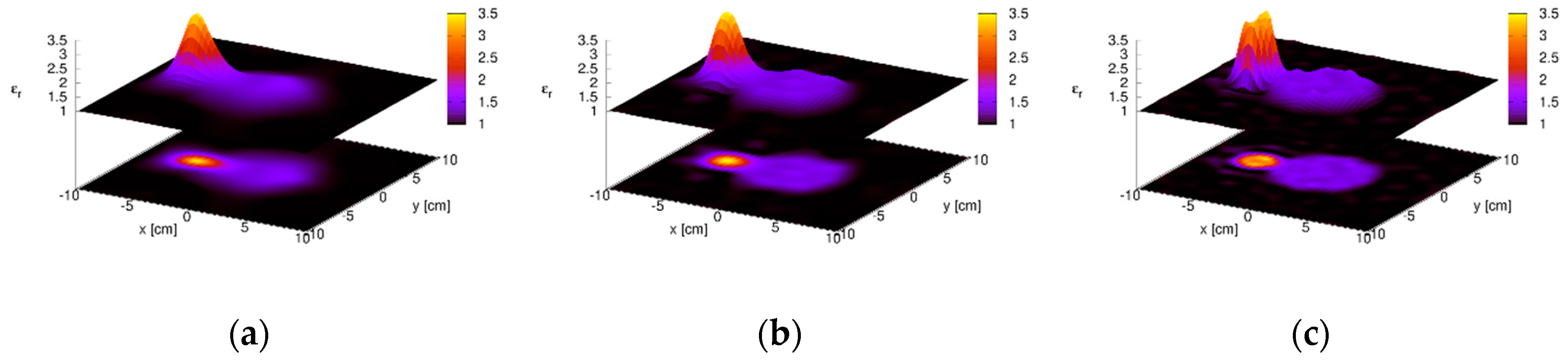
An example of reconstruction obtained by applying the fixed-exponent Lebesgue space inversion procedure presented above is reported here. In particular, the
FoamDielExtTM target from the reference measured data provided by the Institut Fresnel is considered [
39]. Such a target is composed by two adjacent cylinders: The first one has center in (0, 0) cm, radius 4 cm, and relative dielectric permittivity 1.45, whereas the second one is centered in (−5.55, 0) cm, has radius 1.55 cm, and relative dielectric permittivity 3 (in both cases, the electric conductivity is negligible). The object is illuminated by horn antennas located in
positions uniformly spaced on a circumference of radius 1.67 m, and, for each view, the scattered field is collected in 241 points uniformly spaced on an arc of 270° on the same circumference. Data acquired at different frequencies are also available in the range [2–10] GHz, with 1 GHz step. The details of the measurement setup can be found in [
40]. During the inversion procedure, the assumed investigation region is a square domain of side 20 cm, which has been discretized into 63 × 63 square subdomains. The maximum number of outer and inner iterations have been fixed to
and
, respectively. Moreover, to test the approach in optimal conditions, the loops are stopped when the variations of the normalized root mean square error
,
being the actual value of the contrast function, fall below 0.5%.
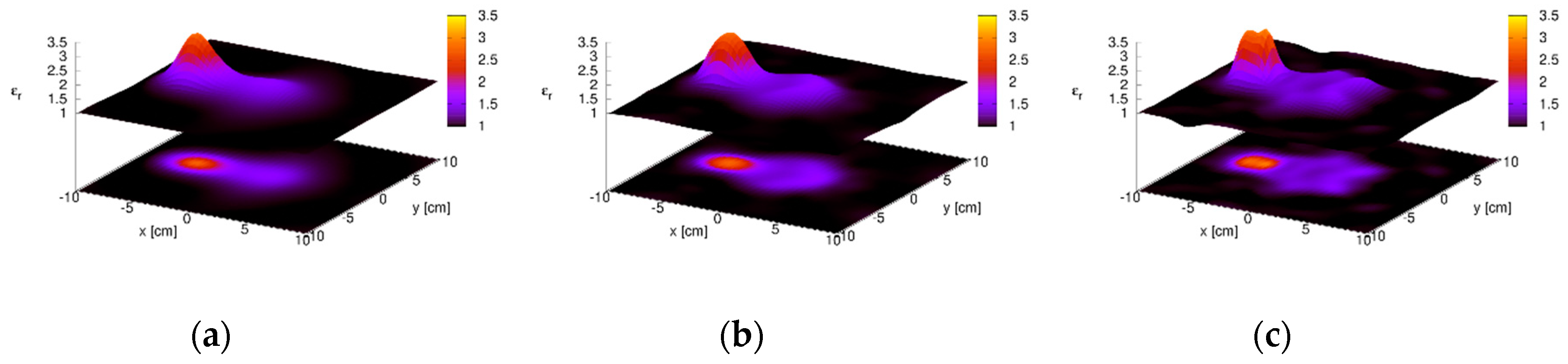
The reconstructed distribution of the relative dielectric permittivity for some of the available working frequencies are shown in
Figure 2. The results obtained with the optimal value of the norm parameter
are reported in the first row, whereas the corresponding Hilbert-space reconstructions are provided for comparison in the second row. As can be seen, the Lebesgue-space method is able to reconstruct correctly the inspected scenario in all cases, providing a quite accurate reconstruction of the cylinders’ cross section, both in terms of dimensions and dielectric permittivity. Using the Hilbert-space procedure it still is possible to identify both targets, but a significant over-smoothing effect is present (which prevents a good reconstruction of the small cylinder) and the ringing in the background is higher. This basic numerical example confirms the behavior of the inversion procedure in
Lebesgue spaces, with respect to different choices of the exponent
parameter, as briefly discussed at the end of the previous Subsection. Indeed, in
Figure 2d–f, where
, oversmooting effects are quite evident, whilst in
Figure 2a–c, where
and 1.3, the reconstructions are less oversmoothed (but some numerical instabilities may occur, especially for smaller
, not shown here). These two kinds of results usually are associated with too high and too low regularization in classical Tikhonov Hilbertian approaches, respectively.
Such considerations are also supported by the values of the mean relative errors reported in
Table 1, defined as:
where
denotes the reconstructed dielectric permittivity, and
,
are the subdomains occupied by the target and by the background, respectively.
Table 1 also reports the computational data for the considered cases (on a computer equipped with an Intel i5-8265u CPU and 16 GB of RAM). Specifically, the numbers of performed outer iterations,
, and the corresponding average computational time per iteration,
, are provided. As expected, the time needed for performing a single outer iteration is similar between the optimal norm and the Hilbert-space approaches. However, in all cases, less iterations are needed when considering the optimal Lebesgue-space procedure, allowing a faster reconstruction.
It is worth remarking that the over-smoothing effect in the Hilbert-space solution can be reduced by varying the regularization parameter, which in the present approach is represented by the number of iterations.
Table 2 reports the reconstruction errors obtained with different values of the parameters
in the case
(the threshold on the
is not set). As can be seen, the object error decreases when higher values of
are used (i.e., a lower regularization is performed), becoming comparable with the ones provided by the optimal value of the norm parameter (in particular, the peak value of the dielectric permittivity is closer). However, the background error increases significantly, producing a greater overall reconstruction error.
As an example,
Figure 3 shows the mean relative reconstruction errors versus the norm parameter
for the case of the lowest frequency (i.e.,
). The overall reconstruction error
presents a minimum value corresponding to the optimal norm parameter
. Following that, the error increases monotonically with
. Moreover, as expected, the background error is always increasing, since low values of
produce sparser solutions. Concerning the object error, in this case a minimum is present at
, and after an initial increase it becomes almost constant. Similar trends can be observed for the other frequencies. To summarize,
Figure 4 shows the behavior of the residual functional (
Figure 4a) and of the normalized root mean square error (
Figure 4b) versus the outer iteration number for the case
. As can be seen, for all values of
the algorithm converges after few iterations (between 5 and 8).


