A Voltage-Based Hierarchical Diagnosis Approach for Open-Circuit Fault of Two-Level Traction Converters

Abstract

This paper proposes a voltage-based hierarchical diagnosis approach for insulated gate bipolar transistors (IGBTs) open-circuit fault of two-level AC-DC-AC traction converters. The proposed approach can diagnose the open-circuit fault in the single-phase rectifier as well as in the three-phase inverter without extra sensors. Moreover, no mandatory control signal injection is required, which ensures safe operation. In addition, the different levels of diagnostic results are flexibly determined by the presented hierarchical diagnosis architecture, which depends on the market requirements of wide use of IGBT modules. To be specific, firstly, a mixed-logic-dynamic estimation model of DC-link voltage is established. Secondly, the diagnosis characteristic function (DCF) is constructed by way of a residual characteristic analysis under normal and various open-circuit fault cases. Thirdly, the vector angular similarity function (VASF) is calculated for leg-level diagnosis and the control signals switching matching method is used to locate the fault in the device-level. Finally, the experimental results show the effectiveness of the proposed approach.

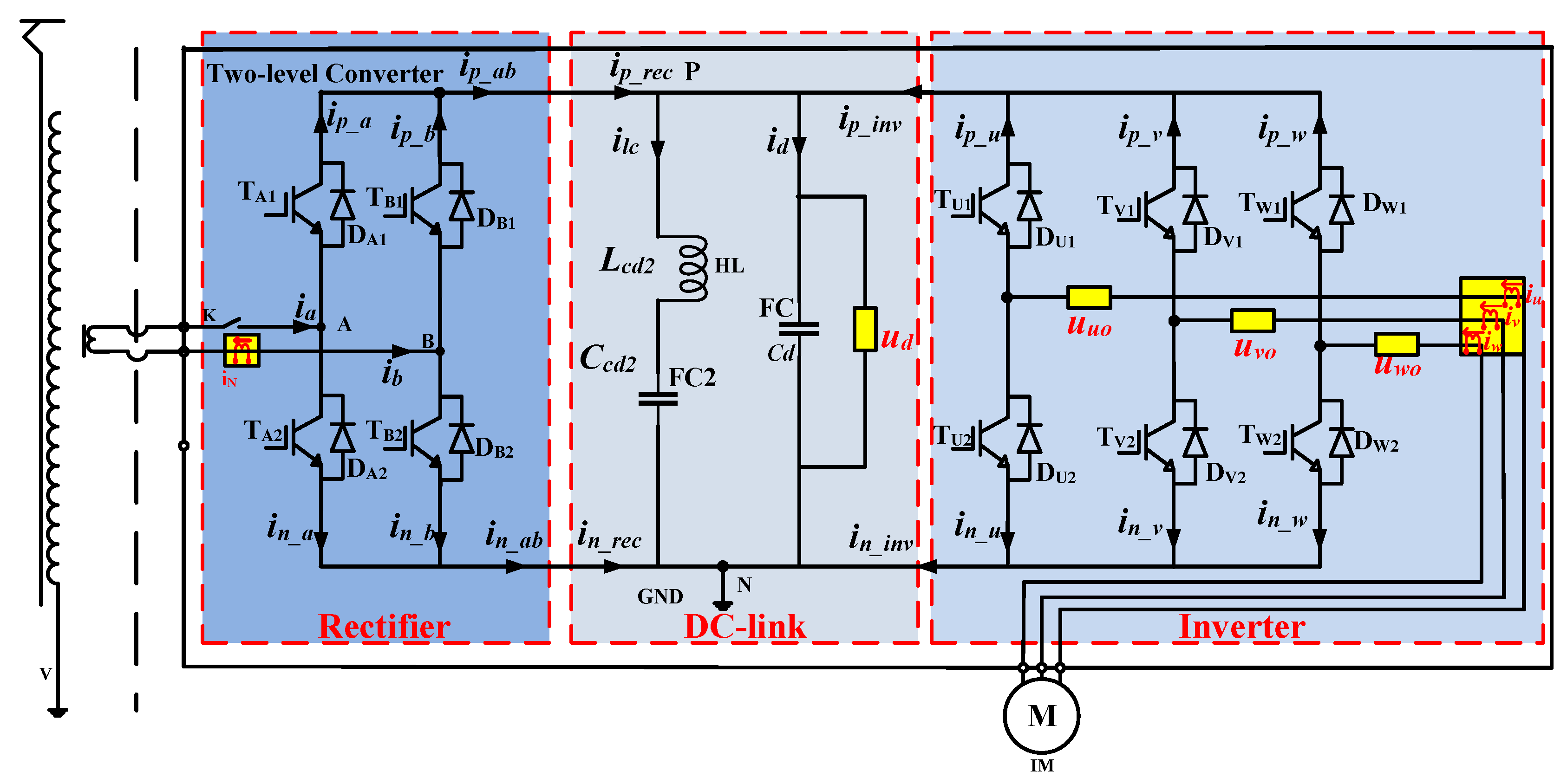
1. Introduction

With the rapid development of railway transportation during recent years, the AC-DC-AC electric traction system is widely applied in electric locomotives and high-speed trains [1,2,3]. As one of the crucial components in the traction system, the traction converters are adopted to provide power and drive the trains forward, which commonly include a rectifier, DC-link circuit and inverter. As a result, once a failure occurs in a traction converter, it will lead to the power performance deterioration of trains and possibly further damage other equipment and even cause catastrophic consequences that threaten the safety of passengers and systems [4,5].

The insulated gate bipolar transistor (IGBT), with its advantage of the ease of driving and higher frequency switching capacities, is widely used in traction applications. According to Reference [4], the IGBT’s failure accounts for 38% of all major components of power converters. Short-circuit fault and open-circuit fault are the two common IGBT failure types [6,7]. Usually, the short-circuit fault has a very short duration and would quickly burn out the IGBT, which finally leads to an open-circuit fault [8]. When the open-circuit fault happens, it may lead to a secondary fault occurrence without immediate diagnosis and fault-tolerance processing [9].

In the existing literature, the diagnosis approaches for the open-circuit fault in converters can be divided into two types—current-based and voltage-based methods [9,10,11,12,13,14,15,16,17]. The current-based methods usually use the voltage monitoring and estimators of the converter. Grid current-based methods are proposed in References [9,11] and the mandatory control signal injection method is proposed to diagnose the IGBTs fault of rectifier, in which some IGBTs are mandatorily constrained to particular switch states to avoid misdiagnosis. It is worth noting that the mandatory injection will increase the diagnostic complexity; more seriously, it will affect the safety of the system’s operation. Although the switching signal isolation is considered in a residual evaluation to avoid mandatory injection in Reference [10]. However, this method actually involves waiting for specific IGBT switch states to replace the mandatory injection which leads to an increase of diagnosis time.

The voltage-based methods mainly concern the voltage measurement in the system. For instance, a pole voltage-based fault diagnosis method is proposed for a two-level AC-DC-AC converter in Reference [12]. In Reference [13], an output line-to-line voltage model-based fault diagnosis technique for a three-phase inverter is proposed. However, the methods mentioned above are unavailable in traction systems. In Reference [14], a DC-Link voltage-based method is proposed, which commonly exists in traction systems and both rectifier and inverter can be diagnosed by this method. However, the specific control signals are needed for mandatory injection, which will lead to a great impact on system operation.

In practical applications, IGBT modules are widely used in traction systems that may contain a two-level or three-level leg or even whole converters [18]. Recently, the research on current distribution and thermal coupling analysis of IGBT modules has become popular [18,19]. However, the literature on fault diagnosis methods mentioned above [9,10,11,12,13,14,15,16,17] mainly consider the diagnosis of a single IGBT. These methods are not only time-consuming but also, when one of the IGBTs in a power module fails, the entire module will need to be replaced. A more flexible diagnostic method is proposed in Reference [14], which divided the diagnosis process into device-level part and leg-level part. In leg-level diagnosis, a Euclidean similarity function is constructed by comparing the Euclidean distance between the residual evaluation function and the current waveform. However, it may cause misdiagnosis near the intersection of different phase currents.

Motivated by the above analysis, a voltage-based hierarchical diagnosis approach for an IGBTs open-circuit fault of two-level AC-DC-AC traction converters is proposed. The proposed approach can diagnose both open-circuit faults in inverter and rectifier with a unified diagnostic architecture and no additional sensors are required. Moreover, the mandatory control signal injection is not required, which will not affect the system’s operation safety. Then, the control signal switching matching process is performed, which can reduce the waiting uncertainty of diagnosis and is further helpful for fast diagnosis in milliseconds. Besides, in order to be suitable for the large-scale application of IGBT modules in the market, the hierarchical diagnosed framework is proposed, including locating the fault at leg-level and device-level.

The rest of this paper is organized as follows. In Section 2, the estimated MLD model of the DC-link voltage is constructed, then the DCF is generated. In Section 3, the faulty features of IGBTs are analyzed. In Section 4, the diagnosis method for the leg-level and device-level is given. In Section 5, the hardware-in-the-loop experiment and results are carried out to validate the effectiveness of the proposed method. Finally, Section 6 gives conclusions.

2. Estimation of DC-Link Voltage and Residual Generation

The topology of an AC-DC-AC two-level converter is shown in Figure 1. It consists of three main parts—a single-phase rectifier of grid-side, a DC-link and a three-phase inverter of motor-side. In more detail, this topology comprises five legs with circuit symmetry; each leg includes two transistors and two diodes. $U_d$ and $i_d$ denote the DC-link voltage and DC-link current, $i_{lc}$ is the secondary filter branch current, $C_d$ represents the supported capacitor value, $U_N$ and $i_N$ are the grid voltage and grid current in the grid-side, $i_a$ and $i_b$ denote the currents of the AC side of the rectifier flows into the A-phase and B-phase leg respectively. Inferred from the circuit structure, $-i_b=i_a=i_N$ . $i_u$ , $i_v$ and $i_w$ denote stator currents of U, V, W phase in the motor-side, respectively.

The two-level converter is a typical hybrid system [9], which includes discrete events like switching signals and continuous variables such as AC-side currents and leg currents. Therefore, the mixed-logic-dynamic (MLD) model [20] is employed to describe the nexus of the terminal currents in each leg and the switching signals of transistors.

The switching functions are defined as

$$\begin{array}{c}\hfill S_x=\left\{\begin{array}{c}1T_{x1}or{D}_{x1}on\hfill \\ 0T_{x2}or{D}_{x2}on\hfill \end{array}\right.,\left(x=a,b,u,v,w\right)\end{array}$$

(1)

The subscripts $x=a,b,u,v,w$ respectively represent the rectifier A-phase, the rectifier B-phase and the inverter U-phase, the inverter V-phase and the inverter W-phase five legs. When the switching function equals 1, the input terminal of the leg is connected to the positive terminal of the DC-link. $S_k$ equaling 0 means the input terminal of the leg is connected to the negative terminal of the DC-link. $T_{x1}$ and $D_{x1}$ express the IGBTs and the diodes in the upper leg respectively, and $T_{x2}$ and $D_{x2}$ express the IGBTs and the diodes in the lower leg respectively as shown in Figure 1.

In general modulation, the relationship among $S_x$, $i_x$ and $s_{x1}$, $s_{x2}$ of a single leg is shown in

Table 1. Relationship between inputs and outputs of a single two-level leg.

${\mathit{i}}_{\mathit{x}}$	${\mathit{s}}_{\mathit{x}1}$	${\mathit{s}}_{\mathit{x}2}$	${\mathit{S}}_{\mathit{x}}$	${\mathit{i}}_{\mathit{x}}$	${\mathit{s}}_{\mathit{x}1}$	${\mathit{s}}_{\mathit{x}2}$	${\mathit{S}}_{\mathit{x}}$
$i_x>0$	0	0	1	$i_x<0$	0	0	0
	0	1	0		0	1	0
	1	0	1		1	0	1

. $s_{x1}$, $s_{x2}$ represent the control signals of IGBTs in the upper and lower legs respectively. There is a total of three possible combinations of $s_{x1}$ and $s_{x2}$ in one leg as shown in Table 1. (a) $s_{x1}$ = 0, $s_{x2}$ = 1. If $i_x$ > 0, $S_x$ = 0, the current $i_x$ will flow through $T_{x2}$; If $i_x$ < 0, $S_x$ = 0, the current $i_x$ will flow through $D_{x2}$. (b) $s_{x1}$ = 1, $s_{x2}$ = 0. If $i_x$ > 0, $S_x$ = 1, the current $i_x$ will flow through $D_{x1}$; If $i_x$ < 0, $S_x$ = 1, the current $i_x$ will flow through $T_{x1}$. (c) $s_{x1}$ = 0, $s_{x2}$ = 0. At this time, the open-circuit fault occurs in an IGBT of this leg. If $i_x$ > 0, $S_x$ = 1, the current $i_x$ will flow through $D_{x1}$; If $i_x$ < 0, $S_x$ = 0, the current $i_x$ will flow through $D_{x2}$. There is a total of ten control signals $s_{x1}$ and $s_{x2}$ output from the system controller, which controls the on-off state of the corresponding IGBTs $T_{x1}$ and $T_{x2}$. The specific analysis of the switch principle of IGBTs and the single leg current path is given in Reference [21].

$$\begin{array}{c}\hfill S_x={\delta }_x\wedge \overline{s_{x2}}+\overline{{\delta }_x}\wedge s_{x1}\end{array}$$

(2)

where − and ∧ represent inversion and AND respectively. ${\delta }_x$ denotes the flag of the polarity of the AC side of the leg. ${\delta }_x$ is a value of ’0’, it indicates a turn-off signal, and when ${\delta }_x$ is a value of ’1’, it indicates a turn-on signal.

The mathematical relationship between each bridge arm of the two-level converter is established as follows:

$$\begin{array}{c}\hfill i_{p\_x}=i_x·S_x\end{array}$$

(3)

where $i_{p\_x}$ denotes the corresponding bridge leg DC side current, when $i_{p\_x}$ is $i_{p\_a}$, $i_{p\_b}$, means the current flowing into the intermediate DC link on the DC side of the rectifier A-phase and rectifier B-phase bridge arm, respectively; when $i_{p\_x}$ is $i_{p\_u}$, $i_{p\_v}$, $i_{p\_w}$, which means U-phase, V-phase and W-phase bridge arm DC side of the inverter respectively.

Relationship between rectifier DC side and AC side current and rectifier switching device state is defined as

$$\begin{array}{cc}\hfill i_{p\_rec}& =i_{p\_a}+i_{p\_b}=i_N·({\delta }_a\wedge \overline{s_{a2}}+\overline{{\delta }_a}\wedge s_{a1})\\ & +(-i_N)·({\delta }_b\wedge \overline{s_{b2}}+\overline{{\delta }_b}\wedge s_{b1})\end{array}$$

(4)

where $i_{p\_rec}$ represents the total current flowing into the DC side of the rectifier. The relationship between inverter DC side and AC side current and rectifier switching device state is defined as

$$\begin{array}{cc}\hfill i_{p\_inv}& =i_{p\_u}+i_{p\_v}+i_{p\_v}=(-i_u)·({\delta }_u\wedge \overline{s_{u2}}+\overline{{\delta }_u}\wedge s_{u1})\\ & +(-i_v)·({\delta }_v\wedge \overline{s_{v2}}+\overline{{\delta }_v}\wedge s_{v1})\\ & +(-i_w)·({\delta }_w\wedge \overline{s_{w2}}+\overline{{\delta }_w}\wedge s_{w1})\end{array}$$

(5)

Kirchhoff’s voltage law gives the DC-link differential equation

$$\begin{array}{c}\hfill C_d\frac{d{u}_d}{dt}=i_{p\_rec}+i_{p\_inv}-i_{lc}\end{array}$$

(6)

It should be noted that

$$\begin{array}{c}\hfill \left\{\begin{array}{c}\frac{i_{lc}}{dt}=\frac{1}{L_{cd}}{u}_{hl}=\frac{1}{L_{cd2}}(u_d-u_{cd2})\hfill \\ C_{cd2}\frac{d{u}_{cd2}}{dt}=i_{lc}\hfill \end{array}\right.\end{array}$$

(7)

where $u_{cd2}$ represents the secondary filter capacitor voltage, $u_{hl}$ represents the secondary filter inductor voltage and $L_{cd}$ represents the secondary filter inductor value, which is the secondary filter capacitor value.

The estimation model of the DC-link voltage is constructed by taking measurements of the actual converter system. When an open circuit fault happens in the actual converter system, it will affect the system measured DC-link voltage through output feedback. Finally, the measured value of the DC-link voltage is compared with the estimated DC-link voltage to generate a residual. The specific steps are given as follows.

Inferred from Equation (7), the relationship model between the DC-ink voltage of the two-level converter, the AC side current of the inverter and the rectifier and the switching state of the switching device are adjusted as

$$\begin{array}{c}{C}_d\frac{d{u}_d}{dt}=i_d=i_{p\_rec}+i_{p\_inv}-i_{lc}\\ =i_N(S_a-S_b)-i_u·S_u-i_v·S_v-i_w·S_w-f\left(u_d\right)\end{array}$$

(8)

where $L_{cd2}$ and $C_{cd2}$ are known quantities, $i_{lc}$ is a variable only related to $u_d$, writing as $f\left(u_d\right)$.

The residual of $u_d$ is defined as

$$\begin{array}{c}\hfill {\tilde{u}}_d\left(n\right)=u_{d\_m}\left(n\right)-{\widehat{u}}_d\left(n\right)\end{array}$$

(9)

where $u_{d\_m}\left(n\right)$ is defined as the measured value in the nth control period of the DC-link voltage of the two-level converter system.

3. Faulty Features Analysis

3.1. Residual Change in Fault Cases

In the normal operation, when the control signals $s_{x1}$ or $s_{x2}$ gives ’1’ (the high-level output), the corresponding IGBT is under the on-state; on the contrary, when the control signals $s_{x1}$ or $s_{x2}$ give ’0’ (the low-level output), the corresponding IGBT is in the off-state. For instance, when $s_{u1}$ gives ’0’, the $T_{u1}$ is in off-state, and when $s_{a2}$ gives ’1’, the $T_{a2}$ is in the on-state, and so on. And $s_{x1}=s_{x1}^{\prime }$, $s_{x2}=s_{x2}^{\prime }$ ($s_{x1}$ and $s_{x2}$ are the control signals generated by the system controller, while $s_{x1}^{\prime }$ and $s_{x2}^{\prime }$ are used to represent the on-off state of the upper and lower IGBTs in x leg respectively and are determined by the control signal acting on them). Thus, the residual signal is close to ’0’. However, when a fault occurs in one of the IGBT open-circuits, then no current flows through the IGBT and this IGBT is always in the off-state, and the corresponding $s_{x1}^{\prime }$ or $s_{x2}^{\prime }$ will turn to a constant in state ’0’. It is worth noting that the on-off state of the faulty IGBT has nothing to do with the control signal after the fault happens, which means no matter what the control signal is, the on-off state of the fault IGBT will always be ’0’, namely the off-state. The residual will change accordingly in certain situations. Furthermore, $S_x^{\prime }$ is defined as

$$\begin{array}{c}\hfill S_x^{\prime }={\delta }_x\wedge \overline{s_{x2}^{\prime }}+\overline{{\delta }_x}\wedge s_{x1}^{\prime }\end{array}$$

(10)

Specifically, according to the residual equation derivation in [21], the Forward-Euler method is used to solve Equation (8). In addition, a basic assumption should be taken into account that the ac side current changes little and is considered a constant in the digital control period $T_c$ [22]. Equation (9) of DC-Link voltage is rewritten as

$$\begin{array}{c}\hfill {\tilde{u}}_d\left(n\right)=\left[\frac{{(-1)}^z·i_x(n-1)·(S_x^{\prime }-S_x)}{C_d}\right]·T_c\end{array}$$

(11)

If $x=a$, then $z=2$, if $x=b$ or $x=u$ or $x=v$ or $x=w$, then $z=1$. According to the switching function of Equations (2), (10) and (11) are further expressed as

$$\begin{array}{cc}\hfill & {\tilde{u}}_d\left(n\right)=\frac{{(-1)}^z·i_x(n-1)·\left[\delta (\overline{s_{x2}^{\prime }}-\overline{s_{x2}})\right]}{C_d}·T_c+\frac{{(-1)}^z·i_x(n-1)·\left[\overline{\delta }(s_{x1}^{{}^{\prime }}-s_{x1})\right]}{C_d}·T_c\hfill \end{array}$$

(12)

When $T_{x1}$ fault, $\overline{s_{x2}^{\prime }}-\overline{s_{x2}}=0$, and when $\delta =0$ and $s_{x1}=1$, then, $s_{x1}^{\prime }-s_{x1}=-1$, ${\tilde{u}}_d$ increases to ${(-1)}^{z+1}·i_x(n-1)·T_c/C_d$; when $T_{x2}$ fault, $s_{x1}^{\prime }-s_{x1}=0$, and when $\delta =1$ and $s_{x2}=1$, then, $\overline{s_{x2}^{\prime }}-\overline{s_{x2}}=1$, ${\tilde{u}}_d$ increases to ${(-1)}^z·i_x(n-1)·T_c/C_d$. The ${\tilde{u}}_d$ in different faulty cases are shown in

Table 2. The ${\tilde{u}}_d$ in different faulty cases.

Faulty IGBT	${\mathit{i}}_{\mathit{x}}>0$	${\mathit{i}}_{\mathit{x}}<0$
$T_{x1}$	−	$s_{x1}=1,{\tilde{u}}_d\left(n\right)={(-1)}^{z+1}·i_x·T_c/C_d$
$T_{x2}$	$s_{x2}=1,{\tilde{u}}_d\left(n\right)={(-1)}^z·i_x·T_c/C_d$	−

.

3.2. Switching Matching Feature

The two-level converter system can be seen as a fast switching system. The control signal has two states include high-level output and low-level output, which means each IGBT has two switch states. In this paper, it is used to locate the IGBT fault in the rectifier. The specific operation method of the switching matching method is reset the control signal with off-signal of each IGBT in turn, before they output to the estimation model, the location of the switching matching mechanism is shown in Figure 2. Then, the switching function of the system estimation model is changed. In order to locate the fault, the idea of the control signal switching matching method is introduced.

For the convenience of fault diagnosis and to avoid the influence of the current direction and the positive or negative residual value to fault diagnosis, the diagnosis characteristic function(DCF) is defined as

$$\begin{array}{cc}\hfill & F\left(n\right)=|\frac{{\tilde{u}}_d\left(n\right)-{\tilde{u}}_d(n-1)}{T_c}|\hfill \end{array}$$

(13)

For analyzing the variation law of the residual in the switching matching process, assuming that $T_{x1}^{\prime }$ or $T_{x2}^{\prime }$ respectively express the upper and the lower faulty IGBT. The control signal $s_l^{"}$ is processed by switching the matching mechanism in Figure 2 and the corresponding switching IGBT expressed as $T_l^{"}$ , which l can be equal to $x1$, $x2$, $y1$ and $y2$. y is not equal to x which express different legs of the rectifier.

As shown in

Table 3. The DCF change of different faulty cases and switching IGBTs.

Faulty IGBT	Switching IGBT	DCF Change	Current Direction	Control Signal
	$T_{x1}^{"}$	$i_x/C_d⟶0$	$i_x<0$	$\left[10XX\right]$
	$T_{x2}^{"}$	$i_x/C_d⟶i_x/C_d$	$i_x<0$	$\left[10XX\right]$
	$T_{y1}^{"}$	$i_x/C_d⟶i_x/C_d$	$i_x<0$	$\left[1010\right]$
$T_{x1}^{\prime }$	$T_{y1}^{"}$	$i_x/C_d⟶i_x/C_d$	$i_x<0$	$\left[1001\right]$
	$T_{y2}^{"}$	$i_x/C_d⟶i_x/C_d$	$i_x<0$	$\left[1010\right]$
	$T_{y2}^{"}$	$i_x/C_d⟶0$	$i_x<0$	$\left[1001\right]$
	$T_{x1}^{"}$	$i_x/C_d⟶i_x/C_d$	$i_x>0$	$\left[01XX\right]$
	$T_{x2}^{"}$	$i_x/C_d⟶0$	$i_x>0$	$\left[01XX\right]$
	$T_{y1}^{"}$	$i_x/C_d⟶i_x/C_d$	$i_x>0$	$\left[0110\right]$
$T_{x2}^{\prime }$	$T_{y1}^{"}$	$i_x/C_d⟶0$	$i_x>0$	$\left[0101\right]$
	$T_{y2}^{"}$	$i_x/C_d⟶i_x/C_d$	$i_x>0$	$\left[0110\right]$
	$T_{y2}^{"}$	$i_x/C_d⟶i_x/C_d$	$i_x>0$	$\left[0101\right]$

, the ’X’ of line ’Control Signal’ means it could be either ’0’ or ’1’, the switching function change in residuals is divided into two cases:

(a) The faulty IGBT corresponds to the Switching IGBT $T_l^{"}$ .

Obviously, after switching the matching operation, the residual change reduced to 0, ignoring the noise.

(b) The faulty IGBT does not correspond to Switching IGBT $T_l^{"}$.

After switching the matching operation, the residual change has no change except in some special circumstances.

According to the above analysis, the method of switching matching is used for fault diagnosis, which can be carried out by judging whether the value of the fault characteristic factor is less than a certain threshold under different switching matching modes. However, there are have been some special cases that may lead to misdiagnosis. As shown in Table 3, one is when $T_{x1}$ fails, if the control signal is [1 0 0 1] and the signal switching position is $T_{y2}^{"}$, and another one is when $T_{x2}$ fails, if the control signal is [0 1 1 0] and the signal switching position is $T_{y1}^{"}$, the value of fault characteristic factors will decline, resulting in misdiagnosis.

To avoid misdiagnosis, the diagnostic factor D is constructed with the value of control signals and the rectifier diagnosis characteristic function (RDCF) which can be expressed as follows:

$$\begin{array}{cc}\hfill & D\left(n\right)=\left|F\left(n\right)\right|·(s_{a1}·s_{b1}+s_{a2}·s_{b2})\end{array}$$

(14)

Different from F, control signals are introduced to the greatest extent to establish D, thus, the false diagnosis can be avoided as much as possible. However, due to limitations, in order to reach the condition that can be diagnosed, that is, D before switching, matching needs to be greater than the diagnostic threshold, which requires a longer diagnostic time. In this paper, the sliding window is used to save the data for a period of time during the rectifier fault diagnosis. The specific operation is described in Section 4 below.

4. Diagnosis Algorithm

The implementation steps of the fault diagnosis method include three parts, fault detection, vector angular similarity-based leg-level diagnosis and switching matching-based device-level fault diagnosis.

4.1. Fault Detection

Firstly, the detection threshold is defined as $h_d$, whose value is determined by a threshold learning method [23], defined as

$$\begin{array}{cc}\hfill & h_d=f_{tlm}\left(\right|R_k{|}_t,h_{d0},K,\alpha ,▵,\epsilon )\end{array}$$

(15)

where $h_d$ is the detection threshold value for diagnosis characteristic function $\left|F\right|$. $f_{tlm}$ is the function of the threshold learning method and includes six variables, which are comprised of the history or training data of detection variables $|R_k{|}_t$, initial threshold value $h_{d0}$, the number of Monte-Carlo simulation K, acceptable false alarm rate $\alpha$, iteration tolerance ▵, and constant $\epsilon$.

Then, compare the DCF which is defined according to Equation (9) with $h_d$ ,if DCF is greater than $h_d$ and lasts for 3$T_c$, an open-circuit fault is detected.

4.2. Vectors Similarity-Based Leg-Level Diagnosis

The vector angular similarity function(VASF) is defined as

$$\begin{array}{c}\hfill J_x\left(n\right)=\frac{|{\sum }_{j=n-m}^{n}C·F\left(j\right)·i_x\left(j\right)|}{\sqrt{{\sum }_{j=n-m}^n[C^2·F^2\left(j\right)]·{\sum }_{j=n-m}^n\left[i_x^2\left(j\right)\right]}}\end{array}$$

(16)

where m is the length of the vector angular similarity. $x=a,b,u,v,w,$ represent the five legs of the converter, respectively. It represents the similarity of two vectors’ directions. The value of 1 for $J_x\left(n\right)$ indicates two vectors, which are in the same or opposite directions. The value of 0 for $J_x\left(n\right)$ indicates two vectors, which are in the orthogonal direction. Obviously, a larger value of $J_x\left(n\right)$ for two vectors indicates more similarity between them.

As can be seen from the above discussion, the VASF of DCF and current flow are established, respectively, to compare the degree of consistency of vector angles of DCF and current flow, so as to locate the bridge arm where the fault occurs.The leg-level diagnosis process can judge the rectifier and inverter faults and also distinguish in which leg of inverter the fault happened. It should be noted that the fault cannot be located in the specific leg of the rectifier because of the special structure of the rectifier, that is, in the case of $x=a$ or $x=b$, VASF shows the same amplitude characteristics.

After fault detection, the VASF of the five legs will be calculated for diagnosis. $J_{max}$ is defined as the maximum of Vector angular similarities, then, judge $J_{max}=J_x$ and last for l$T_c$, the fault is located in the x leg. The diagnostic process is shown in Figure 3.

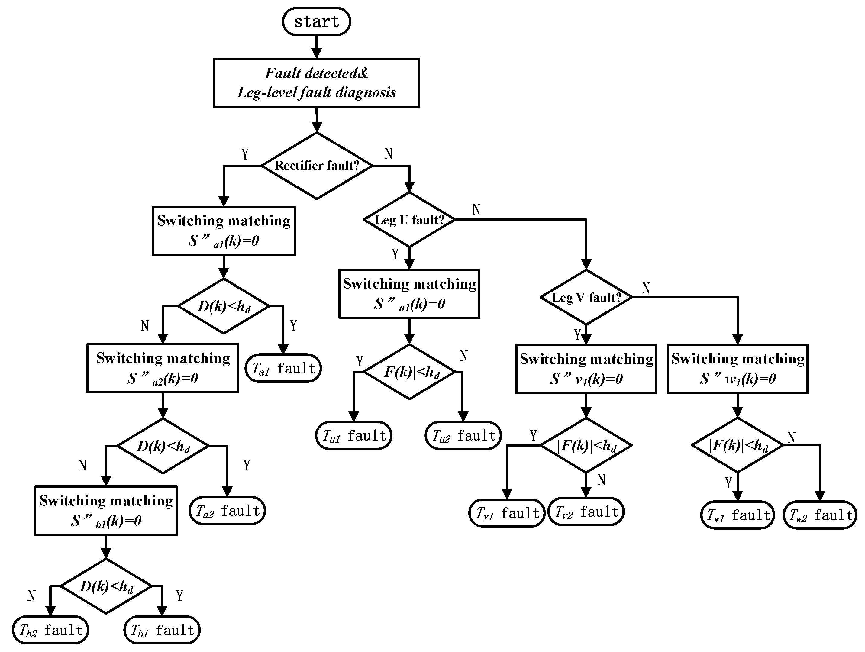
4.3. Switching Matching-Based Device-Level Diagnosis

In the fault location process, the sliding window containing the current, voltage and control signal samples is captured as sliding windows during real-time processing of a certain length L, which is set according to experience to be enough to successfully diagnose the fault location. At kth instant, t is defined as

$$\begin{array}{c}\hfill t=k-L+1\end{array}$$

(17)

The data of the sliding window is expressed as

$$\begin{array}{c}\hfill R\left(k\right)=\left[r\right(t),r(t+1),\cdots ,r(k\left)\right]\end{array}$$

(18)

where R represents one set of the samples inputted into the Estimation Model of DC-link Voltage in Figure 2 and DCF, RDCF, which are written as $U_d\left(k\right)$ , $i_x\left(k\right)$ , $s_{x1}^{"}\left(k\right)$, $s_{x2}^{"}\left(k\right)$ and $F\left(k\right)$, $D\left(k\right)$, and r represents measurements of R. The data of the sliding window is updated as the system runs, in each update the last measurement is dropped and the next measurement is included. The schematic diagram of the sliding window principle is shown in Figure 4.

The sliding window moves its center to the next data sample vector during system operation and when a fault is detected at the nth control period, the sliding window stops moving and the data of the sliding window is saved as $R\left(k\right)$. The position of the sliding window is shown in Figure 2.

The vector angular similarity is constructed above; the leg-level diagnosis can be performed to locate the fault in the rectifier or one phase of the three-phases of the inverter. Then, the fault locating operation of switching matching is carried out; the principle of the switching matching method is described in Section 3.2. The switching matching operations of the inverter and the rectifier differ due to their structural differences, as described below:

(a)

Inverter side: If the fault occurred in U phase of inverter, firstly, the data of sliding window $s_{u1}^{"}\left(k\right)$ are set to 0 by the switching matching mechanism. Then, after model formula calculate, the values of diagnostic factor sliding window $F\left(k\right)$ also changed, according to the first, second row and the seventh, eighth row in Table 3, if the fault location is $T_{u1}^{"}\left(k\right)$ , the data in sliding window will be less than detection threshold $h_d$, if not, the fault location for $T_{u2}^{"}\left(k\right)$ . Similarly, the other two phases of the inverter can be judged. The diagnostic process is shown in Figure 5.

(b)

Rectifier side: Different from the inverter, the current direction of the network side through the two-phase legs of the rectifier is opposite, and the amplitude is the same. Therefore, according to the analysis of the results in Table 3, it can be seen that there are some special conditions that may lead to misdiagnosis. According to this situation, RDCF was established above to locate the rectifier fault. The steps are similar to the inverter but at most two switching matches are required to successfully locate the fault. The specific steps are shown in Figure 5.

5. Experimental Results

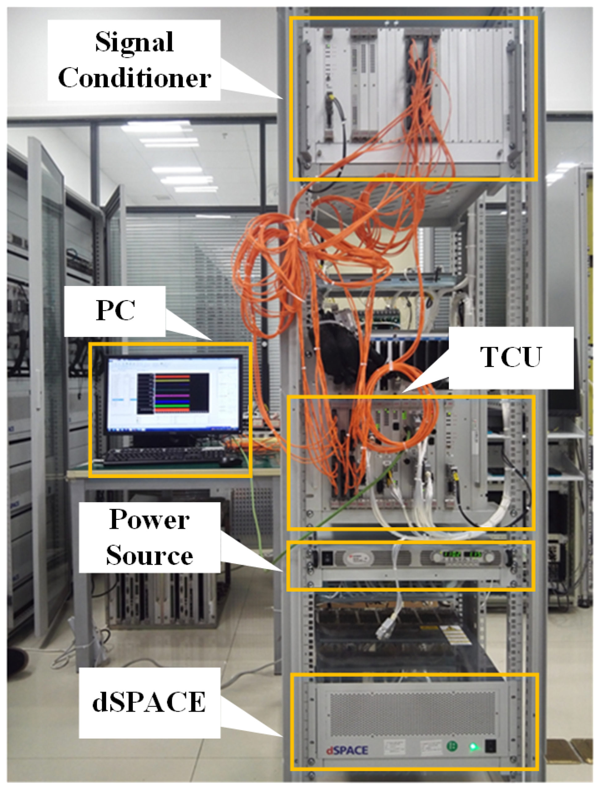
5.1. Experiment Setup

The platform of the experiment is based on hardware-in-the-loop (HIL) [24,25], which has several main parts—a traction control unit (TCU), a dSPACE real-time simulator, host PC, Signal Conditioner and a Power Source, as shown Figure 6. The dSPACE simulator is used to compute the system models with normal and faulty cases and the DS5203 board embedded a Xilinx Kintex 7 field programmable gate array [26]. The control program of the rectifier-side transient direct current control and the inverter-side field-oriented control, as well as the proposed fault detection and diagnosis algorithm, are loaded into the TCU. The signal conditioner is used to convert the signals between the TCU and the simulator. The host PC is used to control the system running and monitors the sensors waveforms in the TCU and the simulator. The control period of the TCU $T_c$ is around 40 $\mathsf{\mu }$s. The main parameters of the platform are from Reference [25].

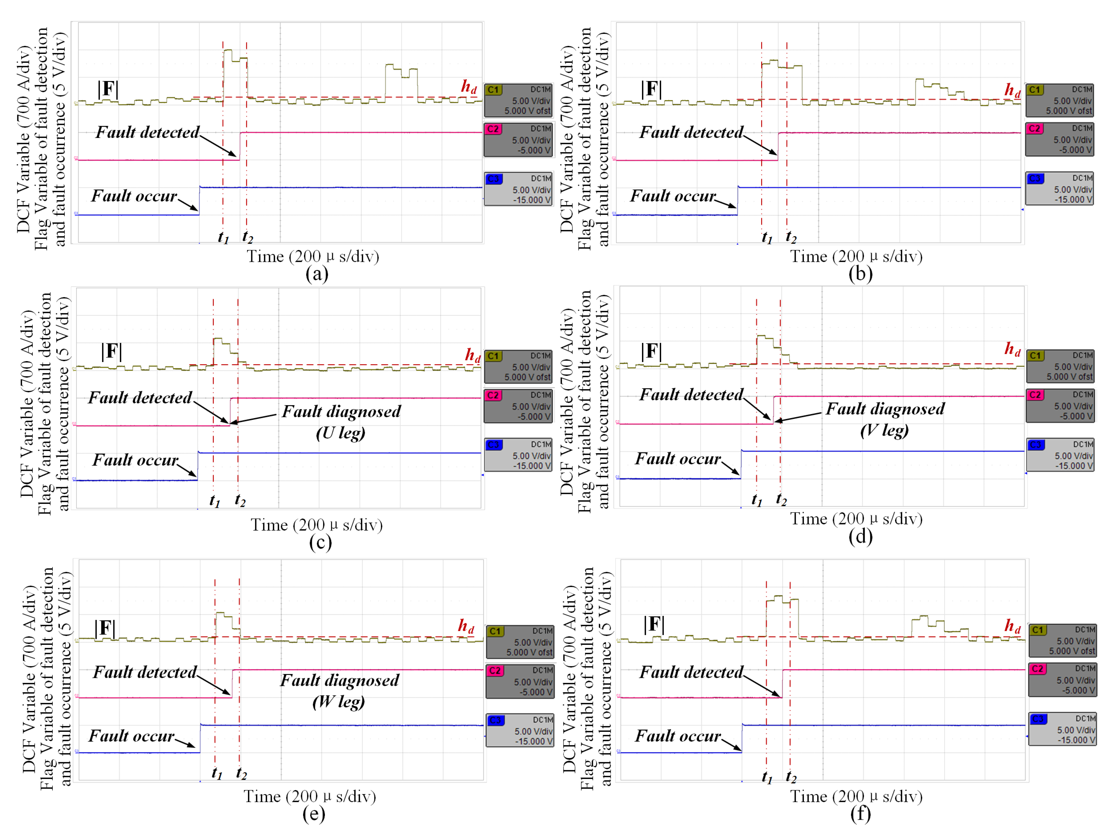
5.2. Fault Detection

When an open-circuit fault occurs, the fault characteristic factor $D\left(k\right)$ will increase, as shown in Figure 7, channel 1. According to the detection criteria, when the total time of fault detection condition ($D\left(k\right)$ exceeds the detection threshold $h_d$) to be satisfied is at least 2$T_c$ during 3$T_c$, then the fault will be detected and confirmed. The detection processes last approximately 120 $\mathsf{\mu }$s. It should be noted that, in Figure 7, the value of DCF did not rise in several control periods after the fault occurred. These periods of time are not included in the fault detection process. This is because, during these periods of time, the current does not flow through the faulty IGBT; at this time, the faulty IGBT will not have any impact on the operation of the system.

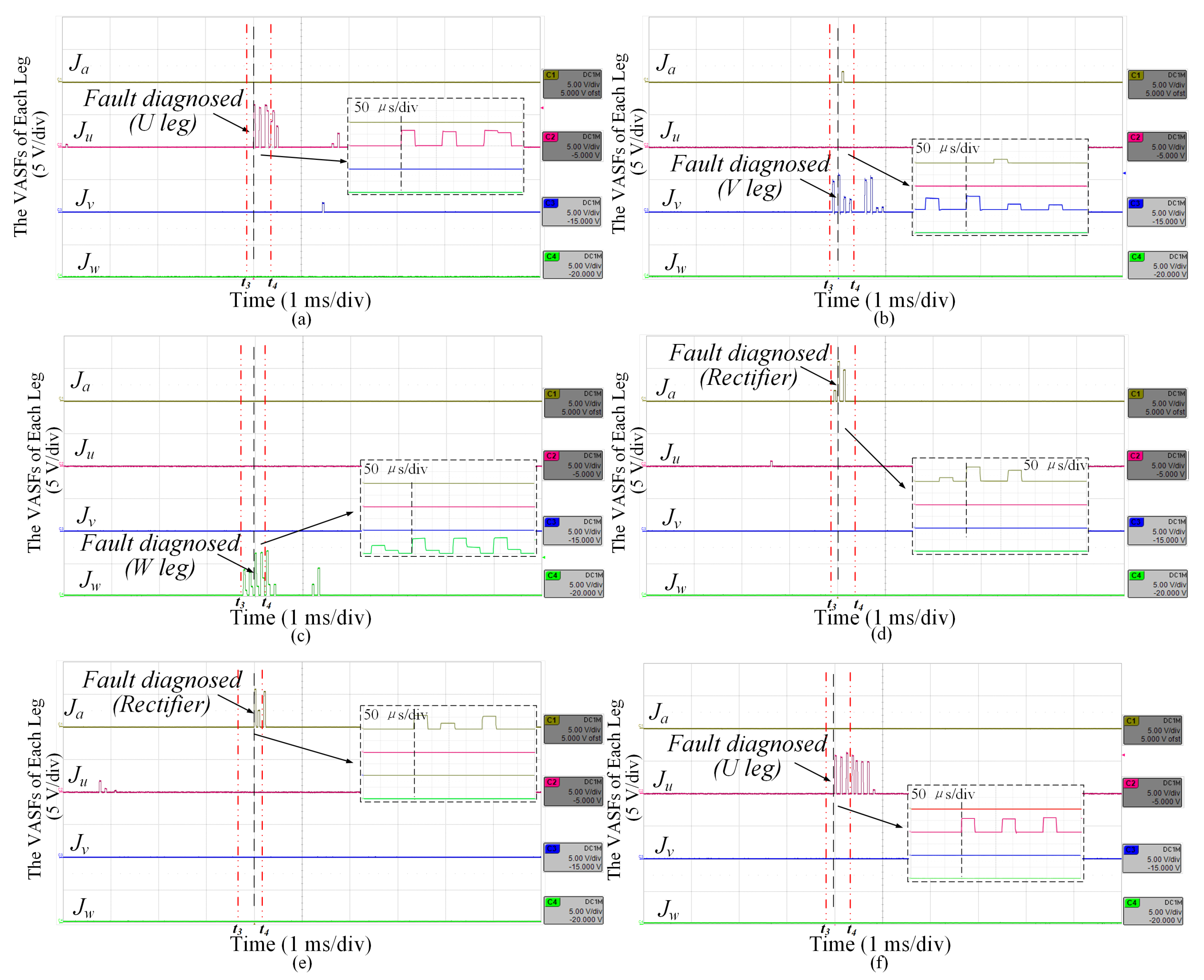
5.3. Leg-Level Diagnosis

Based on the results discussed in Section 4.2 above, VASF shows the same amplitude characteristics whether $x=a$ or $x=b$, then the $J_a$ is omitted in Figure 8. When a fault occurs and the DCF is greater than the threshold $h_d$, then the fault is detected, as shown in Figure 7. At the same time, the value of VASFs rise. Considering that the time for the current to flow through the faulty IGBT is instantaneous, the calculation of VASFs are in real time. Once the fault is detected, the value of VASFs in this control period are judged for leg-level diagnosis. Therefore, the fault detection point and leg-level diagnosis point of the inverter are in the same control period, as shown in Figure 7. The result of the leg-level diagnosis is shown in Figure 8; each small figure of the six figures is the larger one in the $t_3-t_4$ period. The VASF of the faulty leg obviously rises. Because of system noise, other legs also possibly rise while the system runs, thus, each calculation of VASF uses m data to avoid errors, in the experiment, the m is 3.

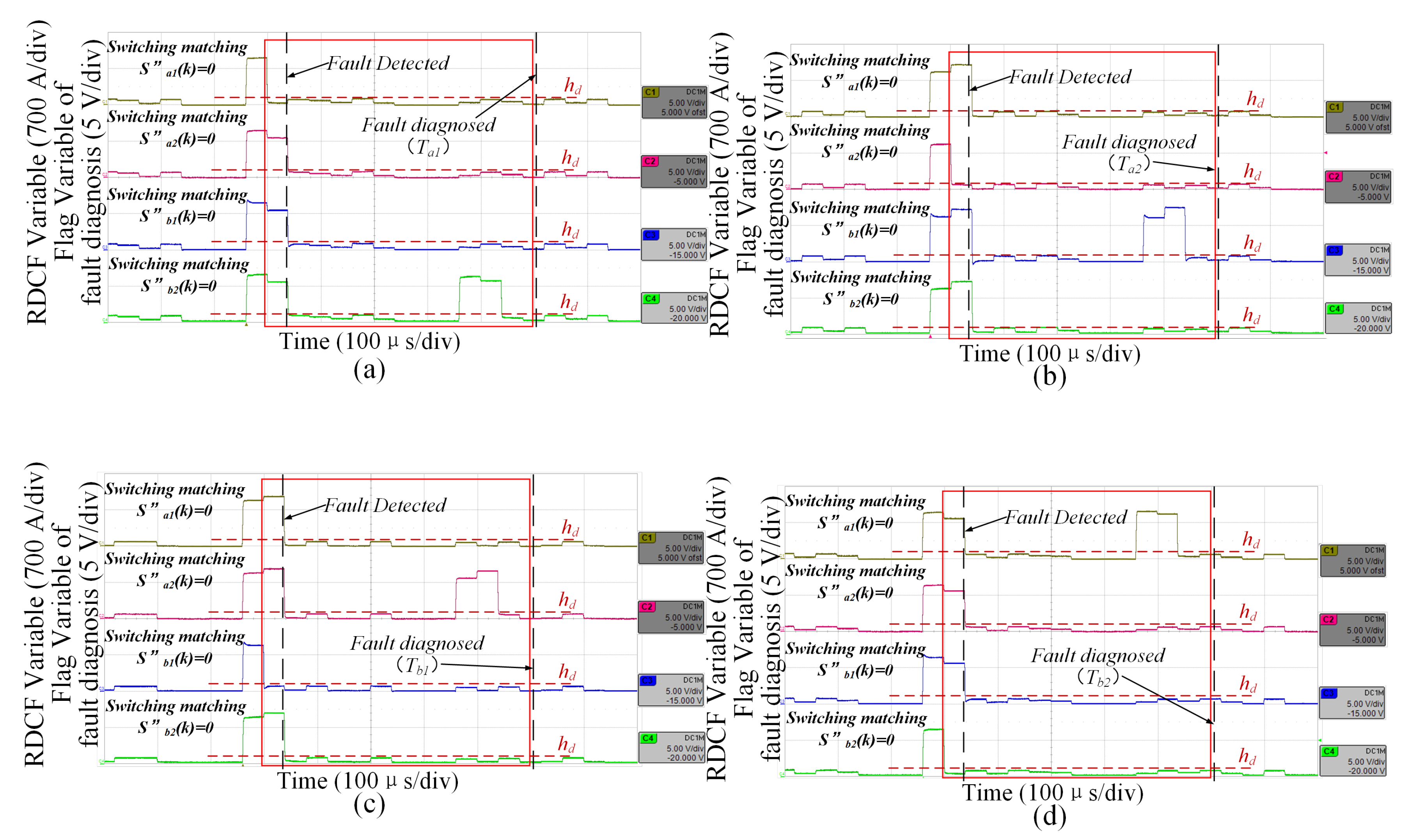
5.4. Device-Level Diagnosis

After the faulty leg is identified, the switching matching operation is performed. Due to the difference of circuit structure between inverter and rectifier, the device-level fault diagnosis is divided into inverter diagnosis part and rectifier diagnosis part. The diagnosis methods are similar but the difference is that, since the fault is located in the leg-level, the inverter diagnosis only needs switching matching of the two IGBTs of the faulty leg, as shown in Figure 9. For the rectifier diagnosis, the four IGBTs of the rectifier need to be switching matched, as shown in Figure 10. The red box is the sliding window and the length of data time saved by the sliding window of the inverter-side is 200 $\mathsf{\mu }$s, and of the rectifier-side is 500 $\mathsf{\mu }$s. It is worth noting that the leg-level diagnosis process goes along with the device-level diagnosis process, thus the length of diagnosis time is inverter-side 200 $\mathsf{\mu }$s and rectifier-side 500 $\mathsf{\mu }$s respectively.

5.5. Comparison with Other Relevant Methods

The comparison of diagnosis performance between the proposed method and relevant methods for back-to-back converters is summarized in

Table 4. The comparison between the proposed method and the relevant methods.

Method	[9]	[11]	[10]	[12]	[14]	Proposed Method
Observation	Currents	Currents	Currents	Pole voltages	DC-link voltages	DC-link voltages
Dignosis time	80 ms	600 $\mathsf{\mu }$s	2.15 ms	10 ms	360 $\mathsf{\mu }$s	620 $\mathsf{\mu }$s
System type of diagnosis	Three-level	Three-level	Two-level	Two-level	Three-level	Two-level
Diagnosis range	Both	Rectifier	Rectifier	Both	Both	Both
Diagnosis independence	Device level	Device level	Device level	Part of Device level	Both	Both
Forced signal injection	No	Yes	No	Yes	Yes	No

. As shown in this table, the proposed method shows good performance. The following performance indices are taken into consideration. The observation (the sensors needed to diagnose), the diagnosis time (maximum time required), the system type of diagnosis (two-level or three-level converters), diagnosis range (rectifier, inverter or both), diagnosis independence (leg-level, device-level or both) and whether a forced signal injection is needed.

6. Conclusions

This paper proposes a voltage-based hierarchical diagnosis approach for IGBTs open-circuit fault in two-level AC-DC-AC traction converters. Firstly, an estimation model of DC-link voltage which includes a fault state is constructed. Then, the diagnosis characteristic function (DCF) is acquired according to the residual of the actual converter system and estimation model, comparing it with the detection threshold for fault detection purposes. Furthermore, the leg-level fault is located by constructing a vector angular similarity function (VASF) and the device-level fault is located by way of a switching matching process. Finally, the experimental results have shown the effectiveness of the proposed method.

By constructing a DC-Link voltage estimation model, both inverter and rectifier can be diagnosed with a unified diagnostic architecture by the proposed voltage-based method. Moreover, compared with the mandatory control signal injection method, the proposed DCF will not affect the system’s performance during the diagnostic process. Then, the model control signal switching matching process is operated, combine the sliding window technique, which can reduce the waiting time caused by certain control conditions of the proposed DCF, which is beneficial for fast diagnosis in milliseconds. Besides, the hierarchical diagnosed framework is proposed to meet the practical demand of IGBT modules widely used in the market, which divides the diagnosed progress into leg-level and device-level.

References

- Blaabjerg, F.; Ma, K. Future on power electronics for wind turbine systems. IEEE J. Emerg. Sel. Top. Power Electron. 2013, 1, 139–152. [Google Scholar] [CrossRef]
- Geng, Z.; Liu, Z.; Hu, X.; Liu, J. Low-frequency oscillation suppression of the vehicle grid system in high-speed railways based on H control. Energies 2018, 11, 1594. [Google Scholar] [CrossRef]
- Chen, Z.; Li, X.; Yang, C.; Peng, T.; Yang, C.; Karimi, H.; Gui, H. A data-driven ground fault detection and isolation method for main circuit in railway electrical traction system. ISA Trans. 2019, 87, 264–271. [Google Scholar] [CrossRef]
- Wang, H.; Liserre, M.; Blaabjerg, F. Toward reliable power electronics: Challenges, design tools, and opportunities. IEEE Ind. Electron. Mag. 2013, 7, 17–26. [Google Scholar] [CrossRef]
- Li, P.; Zhang, C.; Padmanaban, S.; Zbigniew, L. Multiple modulation strategy of flying capacitor DC/DC converter. Electronics 2019, 8, 774. [Google Scholar] [CrossRef]
- Chen, Z.; Ding, X.; Peng, T.; Yang, C.; Gui, W. Fault detection for non-gaussian processes using generalized canonical correlation analysis and randomized algorithms. IEEE Trans. Ind. Electron. 2018, 65, 1559–1567. [Google Scholar] [CrossRef]
- Tao, H.; Peng, T.; Yang, C.; Chen, Z.; Yang, C.; Gui, W. Open-circuit fault analysis and modeling for power converter based on single arm model. Electronics 2019, 8, 633. [Google Scholar] [CrossRef]
- Gou, B.; Ge, X.; Wang, S.; Feng, X.; Kuo, J.; Habetler, T. An open-switch fault diagnosis method for single-phase PWM rectifier using a model-based approach in high-speed railway electrical traction drive system. IEEE Trans. Power Electron. 2016, 31, 3816–3826. [Google Scholar] [CrossRef]
- Ge, X.; Pu, J.; Gou, B.; Liu, Y. An open-circuit fault diagnosis approach for single-phase three-level neutral-point-clamped converters. IEEE Trans. Power Electron. 2017, 33, 2559–2570. [Google Scholar] [CrossRef]
- Xie, D.; Ge, P. Current residual-based method for open circuit fault diagnosis in single-phase PWM converter. IET Power Electron. 2018, 11, 2279–2285. [Google Scholar] [CrossRef]
- Lee, J.; Lee, K.; Blaabjerg, F. Open-switch fault detection method of a back-to-back converter using NPC topology for wind turbine systems. IEEE Trans. Ind. Appl. 2015, 51, 325–335. [Google Scholar] [CrossRef]
- Zhang, H.; Sun, C.; Li, Z.; Li, Z.; Liu, J.; Cao, H.; Zhang, X. Voltage vector error fault diagnosis for open-circuit faults of three-phase four-wire active power filters. IEEE Trans. Power Electron 2017, 32, 2215–2226. [Google Scholar] [CrossRef]
- Shu, C.; Ya-Ting, C.; Tian, Y.; Xun, W. A novel diagnostic technique for open-circuited faults of inverters based on output line-to-line voltage model. IEEE Trans. Ind. Electron. 2016, 63, 4412–4421. [Google Scholar] [CrossRef]
- Yang, C.; Gui, W.; Chen, Z.; Zhang, J.; Peng, T.; Yang, C.; Karimi, H.; Ding, X. Voltage difference residual-based open-circuit fault diagnosis approach for three-level converters in electric traction systems. IEEE Trans. Power Electron. 2019, 1–16. [Google Scholar] [CrossRef]
- Wu, F.; Zhao, J. Current similarity analysis-based open-circuit fault diagnosis for two-level three-phase PWM rectifier. IEEE Trans. Power Electron. 2017, 32, 3935–3945. [Google Scholar] [CrossRef]
- Hong, C.; Chen, W.; Wang, C.; Deng, J. Open circuit fault diagnosis and fault tolerance of three-phase bridgeless rectifier. Electronics 2018, 7, 291. [Google Scholar]
- Chen, H.; Jiang, B. A review of fault detection and diagnosis for the traction system in high-speed trains. IEEE Trans. Intell. Transp. Syst. 2019, 1–16. [Google Scholar] [CrossRef]
- Li, H.; Zhou, W.; Wang, X.; Munk-Nielsen, S.; Li, D.; Wang, Y.; Dai, X. Influence of paralleling dies and paralleling half-bridges on transient current distribution in multichip power modules. IEEE Trans. Power Electron. 2018, 33, 6483–6487. [Google Scholar] [CrossRef]
- Li, H.; Liao, X.; Zeng, Z.; Hu, Y.; Li, Y.; Liu, S.; Li, R. Thermal coupling analysis in a multichip paralleled IGBT module for a DFIG wind turbine power converter. IEEE Trans. Energy Convers. 2017, 32, 80–90. [Google Scholar] [CrossRef]
- Bemporad, A.; Morari, M. Control of systems integrating logic, dynamics, and constraints. Automatica 1999, 35, 402–427. [Google Scholar] [CrossRef]
- Zhang, J.; Peng, T.; Yang, C.; Chen, Z.; Yang, C.; Wen, H. A voltage-based open-circuit Fault Diagnosis Approach for Single Phase Two-Level Converters. In Proceedings of the 2019 International Symposium on Industrial Electronics (ISIE), Vancouver, BC, Canada, 12–14 June 2019; pp. 1737–1742. [Google Scholar]
- Lu, B.; Sharma, S. A literature review of IGBT fault diagnostic and protection methods for power inverters. IEEE Trans. Ind. Appl. 2009, 45, 1770–1777. [Google Scholar]
- Chen, Z.; Yang, C.; Peng, T.; Dan, H.; Li, C.; Gui, W. A Cumulative Canonical Correlation Analysis-based Sensor Precision Degradation Detection Method. IEEE Trans. Ind. Appl. 2019, 66, 6321–6330. [Google Scholar] [CrossRef]
- Yang, C.; Yang, C.; Peng, T.; Yang, X.; Gui, H. A Fault-Injection Strategy for Traction Drive Control System. IEEE Trans. Ind. Electron. 2017, 64, 5719–5727. [Google Scholar] [CrossRef]
- Yang, X.; Yang, C.; Peng, T.; Chen, Z.; Liu, B.; Gui, W. Hardware-in-the-Loop Fault Injection for Traction Control System. IEEE J. Emerg. Sel. Top. Power Electron. 2018, 6, 696–706. [Google Scholar] [CrossRef]
- Peng, T.; Tao, H.; Yang, C.; Chen, Z.; Yang, C.; Gui, W.; Karimi, H. A uniform modeling method based on open-circuit faults analysis for NPC-three-level converter. IEEE Trans. Circuits Syst. II Express Briefs 2019, 66, 457–461. [Google Scholar] [CrossRef]