Abstract
With the rise of Internet of Things (IoT), low-cost resource-constrained devices have to be more capable than traditional embedded systems, which operate on stringent power budgets. In order to add new capabilities such as learning, the power consumption planning has to be revised. Approximate computing is a promising paradigm for reducing power consumption at the expense of inaccuracy introduced to the computations. In this paper, we set forth approximate computing features of a processor that will exist in the next generation low-cost resource-constrained learning IoT devices. Based on these features, we design an approximate IoT processor which benefits from RISC-V ISA. Targeting machine learning applications such as classification and clustering, we have demonstrated that our processor reinforced with approximate operations can save power up to 23% for ASIC implementation while at least 90% top-1 accuracy is achieved on the trained models and test data set.
1. Introduction
Internet of Things (IoT) is the concept of connecting devices so as to improve the living standards of its users by studying the data fed by these devices. In the early examples of IoT, data used to be processed at computationally powerful data centers known as cloud. However, the number of connected devices increases swiftly. Current research shows that even though there were 7 billion IoT devices in 2018, it is estimated that there will be 21.5 billion IoT devices in 2025 [1]. Inefficiency in processing all data on the cloud due to network latency and processing energy have pushed researchers to shift the learning algorithms from cloud to fog which consists of devices that can locally process IoT data [2]. Recent study has shown that even simple learning actions such as clustering and classification can be used for various purposes like abnormal network activity detection [3], IoT botnet identification [4], just to name a few. Embedded machine learning brings down the learning to resource-constrained IoT end-devices.
Employing machine learning algorithms at embedded devices is challenging, because even the simplest algorithm makes use of limited resources such as memory, power budget. Since most IoT end-devices interact with other devices and people, the response time also becomes important, especially when real-time action is required [5]. Hence, in this paper, we propose to include an approximate data-path on the embedded processor to reduce the latency and power consumption overhead of machine learning algorithms on resource-constrained programmable IoT end-devices. Approximate computing [6] is a promising paradigm as it reduces energy consumption and improves performance at the cost of introducing error into its computations. It is beneficial for the applications that can tolerate a predefined error. Machine learning (ML) is clearly one of the applications that benefit from approximate computing. A study on classification in an embedded system shows that erroneous computations do not matter as long as the data points appear in the correct class [7]. In another research, it has been demonstrated that deep neural networks are resilient to numerical errors resulting from approximate computing [8].
Both scientific and commercial attempts exist for designing approximate processors [9,10]. However, none of them is targeted to machine learning applications. The basic novelty in our approach relies on the method that we handle accuracy adjustment. Existing approximate processors correct the precision of arithmetic operations by observing the error at the output of the arithmetic operator. However, this is not the case in our approach. In our processor, the precision of the arithmetic operations is corrected by receiving the feedback from the IoT device user or other components in the IoT ecosystem. A not-too-distant future use case is shown in Figure 1 which depicts a smart cooker. In this scenario, a neural network model for cooking can be stored in the IoT processor or it can be downloaded from the IoT ecosystem such as fog, cloud, or other devices. The cooker senses the ingredients via the sensors (Step 1) and combines them with user preferences to decide on the cooking profile and duration by making approximate computations (Step 2). After the cooking time is over, the food is cooked either properly or not (Step 3). The quality feedback from the user (Step 4) can be done either consciously or unconsciously. In the conscious case, a simple button on the cooker or a home assistant can be used for reporting user satisfaction to the cooker as a feedback. In the unconscious case, the user actions will provide the feedback: If the food is undercooked, the user will ignorantly report the error in cooking by continuing to cook on the stove. If the food is overcooked, then the user will report it to the customer service via a home assistant. In both cases there will be a feedback to the cooker either from the user (undercooked case) or from the customer services via IoT ecosystem (overcooked case). Based on the feedback, the processor will adjust its accuracy level (Step 5). This scenario can be enhanced as follows: During cooking, the energy consumption of the IoT processor on the cooker must be minimized so as to be able to conduct the cooking profile during the cooking period. As a result, reducing the energy by approximating the computations is important. Besides, the processor can be put to sleep time-to-time to monitor the cooking process and make instant adjustments during cooking. It should be noted that quality of service is of extreme important for the IoT products that interact with people. Hence, a low accuracy cannot be tolerated. With our Approximate IoT processor, we observed at least 90% top-1 accuracy on the trained models and test data set.
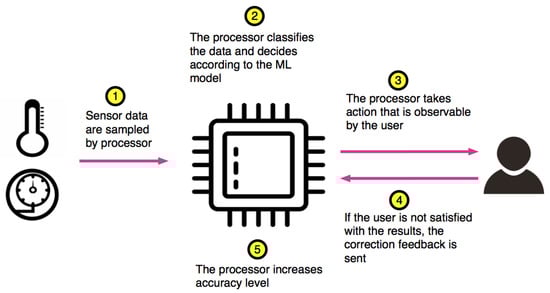
Figure 1.
Precision control proposed in our Approximate IoT processor.
While designing our Approximate IoT processor, we follow a guideline that we derived from various studies in the literature: Firstly, approximate low-power computing at resource-constrained IoT processors needs to be handled at the instruction set level that supports approximate operations [11,12]. Besides, precision of the computations needs to be adjustable to serve different application requirements [6,13,14]. Finally, there should be an application framework support to map user-defined regions of software to approximate computing modules [9]. So, in this paper, we propose an embedded processor, which has approximate processing functionality, with the following properties:
- In machine learning, the majority of operations are addition (ADD), subtraction (SUB) and multiplication (MUL). In our processor, we extend base 32-bit Reduced Instruction Set Computer-V (RISC-V) Instruction Set Architecture ISA [15] only with XADD, XSUB and XMUL for approximate addition, subtraction and multiplication, respectively (Section 3.1). Code pieces that can benefit from approximate instructions are handled via the plug-in that we developed for GCC compiler [16] (Section 4.1).
- We propose a coarse-grain control mechanism for setting accuracy of approximate operations during run-time. In our proposal, number of control signals is minimized by setting each control signal to activate a group of bits. To achieve this, we design a parallel-prefix adder and a wallace tree multiplier. We present three approximation levels to control the accuracy of the computations (Section 3.2).
- To reduce the power consumption, we adjust the size of the operands of the approximate operators dynamically at the data-path. Since approximate operators are faster than the exact ones, dynamic sizing does not deteriorate the performance (Section 3.2.1).
- For monitoring quality of the decisions resulting from the ML algorithms running on our approximate processor, we rely on the interaction of the IoT device with the IoT user or other constituents of IoT ecosystem (Section 2.3).
The paper is organized as follows: Section 2 discusses the similarities and differences between our work and existing studies. The core structure is explained in Section 3. In Section 4 and Section 5, we evaluate our CPU on some classification algorithms on various data sets and discuss our findings. Conclusions are presented in the last section.
2. Related Works
In this section, we will set forth related research under four subsections. We make comparisons between existing approximate processors and our proposal in the first subsection. In the second part, we discuss our approximate adder design with existing methods. In the third subsection, dynamic accuracy control is examined. In the last subsection, we mention about studies that implement clustering and classification algorithms on IoT devices.
2.1. Approximate Processors
In a recent work [11], it has been clearly mentioned that approximate computing at resource-constrained IoT processor still needs to be explored carefully. Proposed implementations of the approximate computing techniques within processors in the literature should be reconsidered in this manner. In [12], approximate building blocks for all stages of the processor including cache exist parallel to the exact blocks. In order to activate approximate operations, new instructions are added in the instruction set. In [17], the data memory is partitioned into several banks so that the memory controller can distribute data to the correct memory bank by observing the output of the data significance analyzer. Though all of these contributions significantly improve the power consumption of desktops or servers, they cannot be used directly in embedded systems due to non-negligible area overhead and cost. In another approach [18], we see approximate data types which should reside in approximate storage. Partitioning a storage for approximate and exact data causes under-utilization of the both partitions. Besides, memory access time dramatically increases due to the software and hardware incorporated in data distribution.
The idea of carrying the approximate operations into action by means of a processor is also realized in [9]. In Quora [9], vector operations are approximately executed, but scalar operations are handled with exact operators. Main hardware approximation methodologies in Quora are clock gating, voltage scaling and truncation. The first method is actually a common low-power technique used in ASIC designs. The second one is also a low-power technique but can also be used in approximation in the sense that voltage can be dynamically lowered too much to diminish the power consumption at the cost of some error. They truncates LSBs to control precision dynamically, but as they stressed in [9], there does not exist a hardware module that calculates results directly in an approximate fashion. They have a quality monitor unit which follow the error rate and truncates LSBs accordingly. In our design, we implement scalar operations with approximate and exact operators which can be selected by software. Separate hardware blocks exist for calculating the result approximately, and controlling the accuracy dynamically. Hence, two designs have different approach in terms of approximate CPU design.
A patented work [10] about an approximate processor design can also be found to show the increasing interest on translating approximate design methodologies into processor systems. Proposed processor in [10] includes execution units, such as an integer unit, a single issue multiple data (SIMD) unit, a multimedia unit, and a floating point unit. Considering a resource-constrained low-power IoT devices, using all of these blocks creates too much area overhead together with an important increase in energy consumption. We simplify architecture of the core by putting execution blocks for only logic and integer operations to minimize power consumption and to make it suitable for resource-constrained IoT end devices. Basic integer addition, subtraction and multiplication operations can be approximately executed via an additional data-path, namely approximate data-path, added to our CPU with small area overhead.
2.2. Circuit-Level Approximate Computing
Approximation at circuit level for adders covers a general implementation flow, which is generating larger approximate blocks by using smaller exact or inexact sub-adders. In [19], 8-bit approximate sub-adders are reconfigured to create 32-bit, 64-bit more efficient approximate designs in terms of critical path delay, area and power consumption. In [20], fixed sub-adders are used to create a reconfigurable generic adder structure. In [21], pipeline mechanism is used to generate an approximation methodology by implementing sub-adders. Using sub-adders can provide a good opportunity to reconfigure the structure and diminish critical path delay to a degree. However, critical path delay can still harm the performance of the operation, especially in high performance applications.
At this point, we believe that proposing an approximation methodology for parallel prefix adders would be useful to implement to reduce critical path length, because these type of adders have a better latency than the others [22]. There is a study in the literature which uses parallel-prefix adders in the approximate adder design [23]. Their approximation method includes precise and approximate parts, but parallel-prefix adders are used only in the precise part. Thus, there is no approximation methodology for parallel-prefix adders. As a result, approximation methodology for this type adders should be investigated to propose energy-efficient ways for high performance and error resilient applications. To address this need, we introduce a simple approximation methodology for parallel-prefix adders which can be further improved for other applications. In our scenario, we specialized the approximate adder to add coarse-grain dynamic accuracy control mechanism. We used Sklansky adder as a case study, which has a moderate area and the best delay among parallel-prefix adders. We control only gray cells in the tree for approximation in order to lower the energy consumption, reduce critical path and still have an acceptable accuracy. This method can be generalized to convert other parallel-prefix adders into approximate ones. For example, Brent-Kung, Kogge-Stone and other parallel-prefix adder structures share the similar structure with Sklansky, hence this idea can also be directly implemented on them.
2.3. Dynamic Accuracy Control
Our approximate processor offers dynamic accuracy control functionality as a programmable feature because each IoT application may require a different accuracy. Fine-grain control as proposed in [14], offers fine tuning of the accuracy at the cost of increased latency, size, and power consumption of the controller. However, applying approximate computing in low-cost and resource-constrained IoT processors should come with no or very little overhead in terms of area while reducing power consumption and lowering the execution time, if possible. Hence, we have preferred to use coarse-grain accuracy control. We create certain power saving levels by putting three approximation levels for each approximate block. Accuracy levels can be adjusted by users or IoT ecosystem in accordance with their power and accuracy requirements as shown in Figure 2. Approximation Level Control Unit can be configured for IoT end devices.
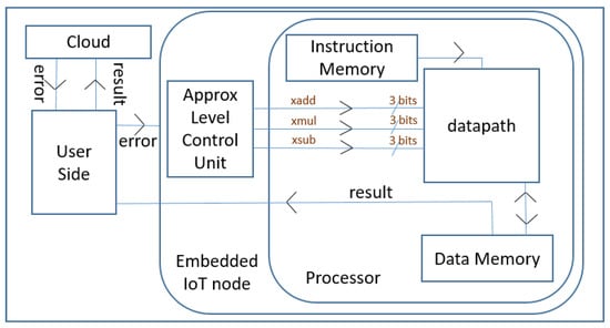
Figure 2.
Flow diagram of dynamic accuracy control in our Approximate IoT processor.
In the literature, dynamic accuracy control is also achieved via dynamic voltage scaling (DVS) [24,25]. There is no dedicated approximate operation block in DVS, the selected parts of the processor are forced to behave inexactly by lowering the supply voltage. In DVS, accuracy control takes longer than a cycle, especially when an accuracy change is required from approximate mode to exact mode. Besides it comes with 9%–20% area overhead in the related studies. In our approach, dynamic accuracy control is applied only on the approximate ALU that is augmented in the data-path. Hence the accuracy control circuit need not be big. Its overhead on the entire CPU is much less than 1% in our design. If we calculate the area overhead due to dynamic accuracy control on each approximate block as calculated in [24,25], then it becomes about 4% at most which is still very small compared to their overhead. Another advantage of our design is that accuracy control takes less than a cycle when switching between different levels of approximation or between one of the approximation levels and exact mode. Since our approximate operators execute faster than the exact ones, dynamic accuracy control circuit does not cause an additional latency.
2.4. IoT Applications
In our CPU, we have specifically focused on classification, clustering and artificial neural network algorithms for ML applications in which Multiply and Accumulate (MAC) loops are densely performed. We have conducted experiments on K-nearest neighbor, K-means and neural network codes to show that an important energy can be saved by our approximate CPU in the ML applications in which these codes are widely used. There are several applications that uses K-nearest neighbor [3,26,27], K-means [28,29] and neural networks [30,31] at IoT devices in such a way that classification, clustering and deep learning processes used in IoT systems can also be carried out on the resource-constrained IoT devices, not only on the cloud. So, an approximate CPU can help them to decrease power consumption while calculating intensive computation loads of these algorithms.
3. Core Description
3.1. General Description of the Core
Our RISC-V core has been developed in C++ and synthesized with 18.1 version of Vivado High Level Synthesis (HLS) tool. Although [32] indicates that HLS is not the best solution to develop programmable architectures like CPUs, we can benefit from HLS tools for fast prototyping of complex digital hardware in a simpler way by using a high-level or modeling language [33]. Hence, our concern in this paper is to study the effects of approximate arithmetic units in the data-path of a processor. We focus on improving the power efficiency for selected ML applications via simply configurable, and adaptable CPU design in which operations can be approximately executed to save power. Our 32-bit core is able to implement all instructions of RV32IM, which is the base integer instructions of RISC-V ISA plus integer multiplication and division instruction sets, except and instructions. This simple core aims specific applications where the operations can be handled by using only integer implementations. We followed a similar approach with Arm Cortex M0 and M3 and did not add a floating point unit (FPU) to reduce area and lower the energy consumption for low-cost IoT devices.
Figure 3 shows the general structure of the core. Execute stage consists of two distinct parts, i.e., exact and approximate blocks, plus conventional exact shifter block. Exact Part perform exact calculations arithmetic and logic instructions. Approximate Part contains XADD, XSUB and XMUL operations, which stand for approximate addition, approximate subtraction and approximate multiplication, respectively. There are not any instructions in RISC-V ISA for approximate operations. New instructions are needed for integrating designed approximate hard blocks to the architecture at instruction level, for the best implementation as stressed in [12]. New instructions, shown in Figure 4, are introduced in such a way that they do not overlap with the existing instructions of the entire RISC-V ISA. Both MUL, SUB and ADD instructions can be converted to approximate instructions by only changing the most significant bit (MSB). This small change also facilitates our work in control unit of the core where the MSB of the instruction is just controlled to determine the operation is approximate or not.
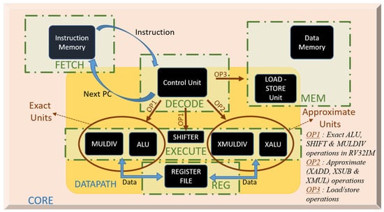
Figure 3.
General flow diagram of the implementations in the proposed core.
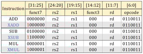
Figure 4.
R-type RISC-V instruction structure and modification for approximate ( XADD, XSUB and XMUL) operations.
3.2. Approximate Units
We introduce new approximate designs for enabling coarse-grain dynamic accuracy configuration and dynamic sizing that we propose in this paper. In approximate module designs, we mainly focus on circuit level approximation, while integrating these blocks with a softcore to execute some chosen instructions in approximate mode will be a kind of architecture level approximation. In our design, the precision of the approximate hardware modules is controlled by approximation levels. Our approximation is based on bypassing selected sub-blocks that exist in the proposed hardware modules. Hence, our approach is different than truncating the least significant bits of the results as applied in [18,34]. Approximate operations of our core are addition, subtraction and multiplication. However, further approximate modules can also be added to the data-path as shown in Figure 5.
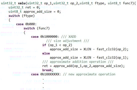
Figure 5.
C code for XALU block in HLS. op_1 and op_2 refer to two operands and XLEN is the length of a register which is 32.
An HLS tool takes the design description in a high-level language as the input and generates the hardware by synthesizing the program constructs to the primitives of the target architecture. HLS provides a fast prototyping and design space exploration for the target hardware. The quality of the design is strongly dependent on the vendor-specific library primitives and user-selected directives that are applied during the code development. Attempting to design an RTL circuit with a high-level language and applying HLS usually produces an inefficient hardware. Hence, approximate adder/subtractor and multiplier of our core are designed with Verilog Hardware Description Language (HDL) instead of C++. However, at the time of writing this manuscript, Vivado HLS does not support introducing blocks designed in HDL to the core designed with a high-level language such as C/C++ [35]. We solve this issue by using stub codes for the functions that correspond to the approximate operations.
In the code given in Figure 5, a C function, namely is defined to conduct the approximate addition/subtraction operation when it is called. However, function only contains stub code. Consequently, the synthesized core contains the synthesized stub codes which we replace by the approximate blocks developed in Verilog. In this way, the system integration is achieved.
We design a dynamically sizeable 32-bit Sklansky Parallel-prefix Adder and a 16 × 16 bit Booth Encoded Wallace Tree Multiplier with Verilog HDL as an exact adder and an exact multiplier. Structural coding style is used in order to facilitate the control of each sub-block more conveniently although it is more difficult to write the codes in this way. These exact blocks are modified to make approximate calculations. Both approximate designs consist of approximate levels which can be individually arranged to act as selective-precision approximate operators at run-time. These approximation levels are stored in registers. Each register can be controlled from a circuit, which is out of the core. Thus, the user or the IoT ecosystem can adjust the approximation levels while the system is running. We give a direct control for these registers that the approximate levels can be controlled independent of the operation. We only put coarse-grained three levels of approximation for each approximate design to create distinct three levels for power saving modes. Dynamic sizing for unused leading zeros of the operands is controlled directly by data-path. A diagram for approximation level control and dynamic sizing flow is shown in Figure 6. Subsections below will describe their dynamically sizeable structure first and then each approximate design separately.
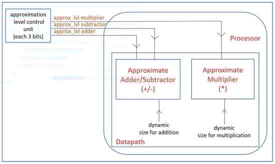
Figure 6.
Flow diagram of dynamic control of the approximation levels and dynamic sizing.
3.2.1. Dynamic Sizing
Data size and dynamically adjustable operations may affect consumed power amount, dramatically, as highlighted in [18]. We considered to adjust the size of our approximate blocks in hardware in accordance with the size of the operands at run-time just before the execution stage to improve power efficiency a bit more. Dynamic sizing produces the minimum size for a block for the exact realization of an operation. Minimum size can be obtained by determining the number of bits that are actively used to represent the values at the operands. We call these bits as active bits. The number of active bits in an operand can be evaluated by subtracting the number of the leading zeros from the register size which is 32 for RV32IM. In Section 4.4.1, we demonstrate that dynamically adjusting the size of the approximate blocks significantly affects the power, but has no effect on the accuracy of the result.
GNU Compiler Collection (GCC) provides function, which can be synthesized by Vivado HLS, to count the leading zeros. After approximate operation is received, the active bits of the operands are determined as shown in Figure 5. Resized operands are processed by the approximate operators that are adjusted accordingly to perform the desired operation more efficiently. It should be noted that there is no dynamic sizing operations for signed negative values as they have no leading zeros. Dynamic sizing operation for signed values requires comparison of the two operands. In case of having negative operands, it is necessary to know which absolute value is greater so as to know whether the result will have leading ones or zeros. Thus, it results in a more complex control mechanism. During our experiments, we found that this complex hardware does not contribute to power reduction. Thus, we use dynamic sizing for operands when they have leading zeroes.
3.2.2. Approximate Adder/Subtractor
In this study, we propose a new approximation methodology for parallel-prefix adders. We designed a 32-bit signed Sklansky adder [36] and modified it for approximate addition and subtraction operation. Parallel-prefix adders create a carry chain by taking Propagate (P) and Generate (G) signals as inputs. P values represent XOR of two inputs calculated for each bit of two operands, and G values AND of each bit of two operands. As shown in Figure 7, each row in the tree includes 32-bit P and G values created by the cells. There are two types of cells, namely black cell and gray cell. Black cell performs ANDOR operation for G value of the next row and AND operation for P value of the next row. The gray cells are used to determine the last values of G bits. Hence there is no need for further computations of P values. As a result, they perform only ANDOR operation to find the last G value for each column. In white cells, P and G are directly buffered to the next row. After all final carry values are obtained, they are XORed with P values calculated from the inputs and final result of the 32-bit addition operation is obtained.
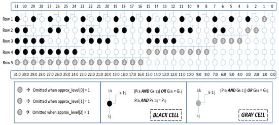
Figure 7.
Sklansky adder tree used for approximate adder design.
We perform approximation on gray cells. In Figure 7, gray cells are the last cells to determine the final G value for a column in the adder tree. Instead of performing this last ANDOR operation of gray cells, they can be omitted for the sake of power efficiency although the final result may be inaccurate. Three approximation levels are defined to control the accuracy. First level omits the gray cells used for the least significant byte. Second level controls the gray cells used for the next eight bits and third level gives the decision about the gray cells used last sixteen bits. It should be highlighted that this operation is different than truncating LSBs [18,34], because we do not remove these bits, instead, we bypass the gray cells and directly use the input value of the gray cells as the tree outputs, hence it still affects the final results.
Subtractor is implemented by negating the second operand and using the same adder block when approximate subtraction (XSUB) operation comes. This provides us an approximate subtractor without consuming any additional resources on chip.
3.2.3. Approximate Multiplier
16x16 bit booth encoded Wallace tree exact multiplier is designed. We computed partial products (PP) as radix-4 booth [37]. After partial products are obtained, Wallace tree structure depicted in Figure 8 is built to sum all partial products. For the CSAs, we used an approximation methodology described in [38] to realize approximate (3:2) and (4:2) compressors. In final adder, designed approximate Sklansky adder are used. So, the same approximation levels and structure are also valid for this multiplier.
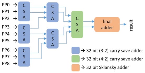
Figure 8.
Wallace tree structure for the summation of partial products. All CSAs and final adder are approximate.
4. Experiments
We synthesized a sample core for Zynq-7000 (xc7z020clg484-1) Field Programmable Gate Array (FPGA) by using Xilinx Vivado HLS 18.1. It can run safely with a clock frequency of 100 MHz. This CPU occupies about 3% of on-chip resources in Zynq-7000 FPGA. Resource utilization on the target FPGA can be seen in Table 1. For memories, we use 40 KB BRAM for instruction memory and 90 KB BRAM for data memory.

Table 1.
Resource utilization in target FPGA for our CPU without approximate blocks.
We implemented some basic ML algorithms on our CPU to evaluate power consumption at the expense of accuracy. Besides, the degree of accuracy loss relative to the amount of saved energy is also important to measure the effectiveness of the design. We chose K-nearest neighbor (KNN), K-means (KM) and artificial neural network (ANN) codes as benchmark algorithms. We executed these codes on our core with different types of datasets to make a proof-of-concept study. We mainly compared the results obtained by running the codes in Exact part with the results in Approximate part. While running this code approximately, we only calculate specific part of the codes approximately, not all ADD, MUL, and SUB instructions as will be explained in Section 4.3. In Approximate Block, we also used different approximate adders and multipliers proposed in literature to show that other approximate designs can also be used in the proposed CPU as approximate unit and different accuracy and energy saving can be obtained from different approximate modules.
4.1. Experimental Setup
The synthesized core including approximate blocks is obtained in Verilog HDL. C codes for the benchmark algorithms are compiled with 32 bit riscv-gcc [16] for exact and approximate For approximate executions, approximate portions are determined and necessary modifications are done on the code as described in the following paragraphs.
To mark approximate regions of code, we have built a plugin for GCC 9.2.0. The plugin adds a number of pragma directives and an attribute. An example usage of this plugin can be seen in Figure 9. The pragma directives are used when only some operations should be implemented with approximate operators as shown in Figure 9a. The attribute, Figure 9b, is helpful for declaring whole functions as approximate.
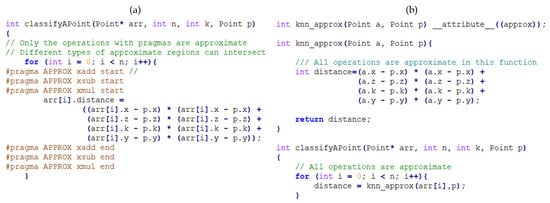
Figure 9.
Implementing KNN by using (a) pragmas and (b) attributes for approximable regions.
The plugin implements a new pass over the code. This pass is done after the code is transformed into an intermediate form called GIMPLE [39]. In this pass, our plugin traverses over the GIMPLE code to find addition, subtraction and multiplication operations. These operations are found as PLUS_EXPR, MINUS_EXPR and MULT_EXPR nodes in the GIMPLE code. The plugin simply checks if these operations are in an approximable region defined by the pragma directives and attributes. If they are, then these GIMPLE statements are replaced with GIMPLE_ASM statements, which are the intermediate form of inline assembly statements in C. The replacements done are shown in Figure 10. Because we set the “r” restriction flag in the inline assembly statements, which hints the compiler to put the operand into a register, non-register operands of an operation (e.g., immediate values) are automatically loaded into registers by GCC.

Figure 10.
Replaced assembly statements for XADD, XSUB and XMUL in GIMPLE.
riscv-binutils [40] provides a pseudo assembly directive “.insn” [41] which allows us to insert our custom instructions into the resulting binary file. This directive already knows some instruction formats. So we choose to have an R-type instruction with the same opcode as a normal arithmetic operation. In our implementation, funct3 field is always zero and funct7 has its most significant bit flipped. We enter these numbers and let the compiler fill the register fields itself according to our operands.
We used riscv-gnu-toolchain [42] to test this plugin and verified its functionality. After achieving the specialization of the compiler for our approximate instruction, we can directly use the machine code created by this compiler in our core.
For accuracy measurement, exact benchmark codes are executed by using behavioral simulator of Xilinx Vivado HLS. The files that contain the results of exact executions are regarded as the golden files. Then, the same codes are executed on the synthesized core to verify that its results are the same with the ones in the golden files. Then approximate codes are run on the synthesized core and the results are compared with the true results in the golden file and the accuracy is computed. Accuracy metrics here is top-1 accuracy which means that the test results must be exactly the expected answer. Let n denote the number of tests carried out in both exact CPU and approximate CPU, which uses approximate operators only in the annotated regions. Approximate CPU tries to find exactly the same class as the exact CPU model finds. We compare all the results obtained from both parts for n tests and the percentage of matching cases in all tests gives us the accuracy rate. Simulations are performed in Xilinx Vivado 18.1 tool and a Verilog testbench is written to run the tests and write the results into a text file automatically for each case.
Power estimation results are obtained with Power Estimator tool of Xilinx Vivado 18.1. For the best power estimation with a high confidence in the tool, post implementation power analysis option with a SAIF (Switching Activity Interchange Format) file is obtained from the post-implementation functional simulation of the benchmark codes.
In experiments, we report dynamic power consumption on the core, because the main difference between the exact and approximate operation can be observed with the change in the dynamic activity of the core. We omit static power consumption, because we realize that static power consumption in the conventional FPGAs mainly stemming from the leakages that are independent of the operation. On the other hand, due to domination of static power in FPGA, it may not be convenient to design final product as an FPGA, hence presented power savings here are just to verify the idea. An ASIC implementation where static power is negligible (<1%) may be more beneficial to save significant total power in these applications. To see the difference, an ASIC implementation results are also presented in Section 5.1.
TSMC 65 nm Low Power (LP) library and Cadence tools are used to synthesize our core for ASIC implementations. We have used TSMC memories for our data and instruction memories with the same sizes as in our FPGA design. We calculate the power consumption with the help of tcf file, which is similar to SAIF, created from the simulation tool to count toggle amounts of the all signals.
4.2. Datasets and Algorithms
KNN, KM and ANN algorithms are implemented with different datasets to observe the change in the results in accordance with the data with different lengths and attributes. Three datasets are chosen from UCI Machine Learning Repository [43]. In total, we have five datasets obtained from three different sources of the given repository as shown in Table 2.
Table 2.
Implemented datasets and their properties.
KNN is one of the most essential classification algorithms in ML. Distance calculations in KNN are multiply-and-accumulate loops that are quite suitable to implement approximately. KNN is an unsupervised learning algorithm. However, we put some reference data points with known classes into the data memory so that incoming data can be classified correctly and in real-time. K parameter in KNN which is used to decide group of the testing point is defined as three for all datasets. We followed the same approach for KM, which is a basic clustering algorithm. In KM, k-value, which determines how many clusters will be created for the given dataset, is chosen as the number of the class in the datasets. Our last algorithm is ANN which is also very popular in ML. We trained our ANN models with our datasets and obtained weights for each dataset. Then we used these model weights and the model itself in our code. In ANN algorithm, the input number is the attribute number of the used dataset, 4 and 7, hidden layer is one which has two units for the datasets that have four attributes, and four units for the datasets that have seven attributes. Two units for the output layer are used to determine the classes of the test data. Loop operations in all layers of neural network are operated approximately to make case study for our work.
4.3. Approximate Regions in the Codes
In this study, we have specifically focused on classification, clustering and artificial neural network algorithms for ML applications in which multiply and accumulate (MAC) loops are densely performed. We also add subtraction operations in the same loops to carry the idea of the approximate operation one step further when it is possible. It is worth to note that we are not doing any approximate operation for datasets as proposed in [18]. We can create approximable regions in the code with the help of pragma and attribute operations in C as we previously mentioned in Section 4.1. Hence, we can decide which regions should be approximated in the codes at high level. In KNN and KM, approximate operations are only implemented on the specific distance calculation loops that contains addition, subtraction and multiplication operations in each iteration. An example of approximable region creation in KNN code can be seen in Figure 9. As it can be seen from the given codes in Figure 9a, we only calculate the operations for distance calculation in the loop approximately, not the addition and compare operations for the loop iteration &. Figure 9b does exactly the same thing as part (a), because knn_approx, which is the body of the loop in classifyAPoint, is approximated with an attribute. Both approaches have their own advantages. Approach in part (a) enables the application developer to selectively decide on the approximate operations. For example, the application developer may want to use approximate addition and subtraction but exact multiplication. In that case, the pragmas due to approximate multiplication should be removed. Approach in part (b) helps the application developer to use all approximate operators available in the processor. It should be noted that, in ANN experiments, weight calculations contains only addition and multiplication operations. Thus, we confined our approximation level only to addition and multiplication in this code. That is the reason why we can observe the impact of the approximate subtraction operations on the power consumption in only KNN and KM tests.
4.4. Experiments
4.4.1. Dynamic Sizing
First experimental point is to measure the effect of dynamic sizing on the power consumption. To see the effect of dynamic sizing on power saving, we set approximation level of the approximate operators as zero which means that the operations are realized as if they are running at the exact part. Hence, accuracy is not studied in this part. Table 3 shows that dynamic sizing can provide up to 12.8% power savings. Here, refers to the case when approximate operation is confined to addition but the approximate adder is running in exact mode. The same approach is followed for our approximate multiplier, . Finally, represents when both of the approximate operators are running in exact mode with only dynamic sizing operation is activated. As we discussed before, there is no dynamic sizing operation for the subtraction and signed operations.
Table 3.
Contributions of dynamic sizing to the power saving percentages of the new approximate blocks, given as the average and maximum of the results from different datasets for each algorithm.
4.4.2. Approximate Addition/Subtraction and Exact Multiplication
In this part, we have confined the approximate operation to the approximate addition and subtraction with XADD and XSUB, and executed multiplication on the exact multiplier with MUL instructions. We also tested another approximate adder from the literature. We used 32-bit AA7 type of adder in DeMAS [44], which is an open source approximate adders library designed for FPGAs. We obtained two approximate adders from AA7: , has 28 exact and 4 approximate bits. has 24 exact and 8 approximate bits. In our design represents only approximate addition and refers to approximate addition and subtraction operations that are implemented on our adder design. Approximation level of our adder is modified according to the bit-length of the datasets. For 8-bit datasets, it is 2 and for 16-bit, it is 3. Then, we obtain four approximate modules. These blocks actually cause area overhead on the CPU. The area overhead for , and is reported as 2.2%, 2% and 3.5%, respectively. Area overhead for is the same with , because it uses the same design. The accuracy of the results and the percentage of power gain compared to the operation implemented fully on Exact part are given in Table 4.
Table 4.
Accuracy and power saving percentages of the approximate blocks, given as the average and maximum of the results from different datasets for each algorithm.
4.4.3. Exact Addition/Subtraction and Approximate Multiplication
In this part, we have confined the approximate operation to the approximate multiplication with XMUL and executed addition and subtraction on the Exact Part with ADD and SUB instructions. Two 16 × 16 bits approximate multipliers, and , are chosen in SMApproxLib [45] which is an open-source approximate multiplier library designed for FPGAs by considering the LUT structure and carry chains of modern FPGAs. Approximation level of our multiplier is again 2 for 8-bit dataset, 3 for 16-bit dataset. Our multiplier design, , together with these two multipliers are added to our core and target ML codes with chosen datasets are separately run on the system. , and create 8.4%, 8.7% and 9.3% area overhead for the design, respectively. Test results are shown in Table 4.
4.4.4. Approximate Addition and Approximate Multiplication
In this part, We used XADD, XSUB and XMUL together to observe the maximum power gain and the quality of results. and are combined as , while and are used together and marked as . Our approximate modules are also combined as , and , they are used together with two different combinations, approximate addition and multiplication, and approximate addition, subtraction and multiplication, to show the improvement in terms of power. The results can be observed in Table 4. , and have 10.6%, 10.7% and 12.8% area overhead, respectively. All area overheads are shown in Table 5.
Table 5.
Resources for approximate blocks and their area overhead on the CPU.
4.4.5. Approximation Level Modification at Run-time
The last experiments are about changing the approximation level while codes are running on the CPU. In previous experiments, we fixed the approximation level for the whole codes, but in this part we split each experiment into three equal parts. In the first part, the codes begin with the first approximation level. In the second, we set the approximation level to two while codes are running. When the last interval comes, the approximation level is set to three. These experiments will show us whether we can save power or not for dynamically controllable (programmable) approximations. The results shown in Figure 11 verify that changing the approximation level dynamically in the course of execution does not give too much overhead on our system, and it can give the similar accuracy and power saving rates with the other experiments that we fixed the approximation level. These experiments are implemented in only our designs due to inability to control the other designs in this setup. Figure 11 gives the average results for all codes implemented with 16-bit datasets.
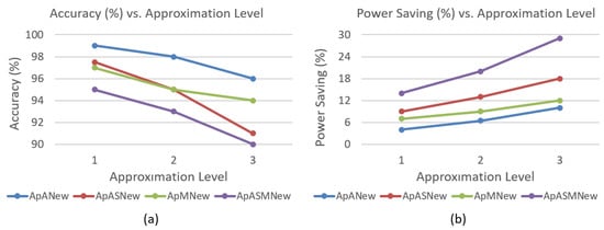
Figure 11.
Approximation level modification at run-time (a) accuracy and (b) power saving results.
5. Discussions
Test results are shown in Table 3 and Table 4 in terms of averages of the results obtained from different datasets for a specific approximate block type. We also add maximum power savings to the tables to indicate the utmost power saving point reached in these experiments.
As seen in Table 4, approximate adders usually gives the best accuracy of the result with the least power gain. We have observed that, in KNN and ANN, using longer dataset can provide better accuracy because of having more reference data in the data memory. In KM this relation become reverse due to the more points needed for the clustering process. Accuracy of the ANN is generally the lowest accuracy achieved with the same dataset and the same adder, because the longest datasets which have 2000 points may still not be large enough to yield the best result from the ANN algorithm. Longer data has also good impact on the improvement in power gain, because increasing the amount of the data leads the MAC loops to dominate the codes, hence most of the running time is covered by these operations which are performed approximately. Generally, datasets with lower bit-length may be less accurate due to the difficulties of the convergence in smaller intervals for approximate calculations. It may also provide less power saving percentage, because used hardware blocks may be much smaller than the longer one, however it still depends on the length of the dataset and approximate adder type.
provides the best power saving rates with almost fully accurate results for almost all cases in the approximate addition and exact multiplication operations. and provides a good example of accuracy and power efficiency trade-off. gives very accurate results with less power saving, but may improve the power efficiency significantly with tolerable error rate which may be more desirable. Making subtraction operations also approximate has yielded an important power saving. can save power up to 24.3% which can be regarded a dramatic power improvement without having an extra subtraction block.
Approximate multipliers reduce power more than the adder because of the fact that the multiplier hardware blocks are generally much bigger than the adders. However, the accuracy of the results are generally worse than the adder case, since the possibility of the large deviation from the real result is higher in the multiplication process. It is possible to reach 18% power saving together with the 95% accuracy rate. Bit-length of the data and the number of data in the dataset are observed to have an effect on the accuracy and the power consumption similar to the approximate adder cases. generally provides the best accuracy for all cases together with the best power saving rates.
The last case where both addition and multiplication are approximately executed provides the most power efficient design at the expense of accuracy loss, as expected. Table 4 shows that the approximate calculations can provide important power savings up to 40.3% together with a quality loss which depends on the approximate adder, algorithm and dataset. For and , average accuracy is above 90% for all codes, while average power saving is above 20% for all cases.
5.1. ASIC Implementation of the Proposed System
Basic disadvantage of the implementations in FPGA for low power applications is static power. In our case, static power is responsible for about 65% of the total consumption. If we include static power in the calculations, power saving becomes 14% at most which can also be considered as an important save, but not enough to say that final target for this design should be an FPGA. Hence, we also synthesized our designs with TSMC 65 nm Low Power (LP) library on Cadence tools. Power consumption of the system for ASIC synthesis is reported in Table 6. In ASIC, 23% of the power can be saved while the accuracy rate is above 90% and static power is less than 1%. Power saving for ASIC design can be further improved by implementing other low power techniques like dynamic voltage scaling and clock gating.
Table 6.
Approximate blocks and their power saving for ASIC implementation.
5.2. Bit-Truncation in the Approximate Blocks
Bit-truncation is a significant way to save energy, especially when it is used for floating point units [18,34]. However, truncation at integer units affect accuracy more dramatically than floating point operations. To see the effect of bit truncation instead of omitting gray cells, we have performed tests without changing our approximate level control circuit. When first level bits are truncated, accuracy drops to less than 15% with a power saving of more than 30%. When the second level bits are truncated, accuracy drops 5% with a power saving of more than 50%. The best case is achieved when the approximation level is set to 1. In this case, the accuracy is less than 45% and power saving is less than 18%. This error rate is too high and energy saving is moderate compared to our design. Hence, it turns out to be inconvenient to implement bit truncation in our system. However, bit-truncation approach may give better results when bit-by-bit fine control is adopted. A new hybrid approach may be a future work to develop a more efficient design. Coarse-grain approximation levels with fine control bit-truncation inside of these levels can be discussed to implement a new proposal.
6. Conclusions
In this paper, we propose and demonstrate the design of an approximate IoT processor. As it is shown in Figure 5, the design is flexible enough to add new approximate operators though our current processor includes approximate blocks only for addition, subtraction and multiplication operations. We try to give an approximate methodology for parallel-prefix adders and make a case study on Sklansky with a coarse grain dynamic precision control. We use the same adder for enhancing an approximate multiplier proposed in the literature. Combining with dynamic sizing of the operands during execution time, we achieve significant dynamic power savings, up to 40.3%, in the conducted experiments. Experimental results point out that 30% of overall power savings are obtained by dynamic sizing idea introduced in this study. Though more versions of dynamic sizing can be proposed, we believe that it should be used carefully so as not to deteriorate the performance and exceed power/area constraints of the IoT end-device. ASIC implementation of the core are also demonstrated. In ASIC implementation, power can be saved up to 23% and static power, which dominates in FPGAs, can be decreased below 1%.
Author Contributions
Conceptualization, A.Y. and İ.T.; methodology, A.Y. and İ.T.; software, M.K. and İ.T.; validation, İ.T.; formal analysis, İ.T.; investigation, A.Y. and İ.T.; resources, İ.T.; data curation, İ.T.; writing—original draft preparation, A.Y. and İ.T.; writing—review and editing, A.Y. and İ.T.; visualization, İ.T.; supervision, A.Y.; project administration, A.Y.; funding acquisition, A.Y. All authors have read and agreed to the published version of the manuscript.
Funding
This research was funded by the Turkish Ministry of Science, Industry and Technology under grant number 58135.
Acknowledgments
We would like to thank Mehmet Alp Şarkışla, Fatih Aşağıdağ and Ömer Faruk Irmak for giving us technical support in designing core structure and helping us to conduct the experiments.
Conflicts of Interest
The authors declare no conflict of interest. The funders had no role in the design of the study; in the collection, analyses, or interpretation of data; in the writing of the manuscript, or in the decision to publish the results.
References
- Lueth, K.L. State of the IoT 2018: Number of IoT Devices Now at 7B—Market Accelerating. Available online: https://iot-analytics.com/state-of-the-iot-update-q1-q2-2018-number-of-iot-devices-now-7b/ (accessed on 23 December 2019).
- La, Q.D.; Ngo, M.V.; Dinh, T.Q.; Quek, T.Q.; Shin, H. Enabling intelligence in fog computing to achieve energy and latency reduction. Digit. Commun. Netw. 2019, 5, 3–9. [Google Scholar] [CrossRef]
- Su, M.Y. Using clustering to improve the KNN-based classifiers for online anomaly network traffic identification. J. Netw. Comput. Appl. 2011, 34, 722–730. [Google Scholar] [CrossRef]
- Doshi, R.; Apthorpe, N.; Feamster, N. Machine Learning DDoS Detection for Consumer Internet of Things Devices. In Proceedings of the 2018 IEEE Security and Privacy Workshops (SPW), San Francisco, CA, USA, 24 May 2018; pp. 29–35. [Google Scholar] [CrossRef]
- Siewert, S. Real-time Embedded Components and Systems; Cengage Learning: Boston, MA, USA, 2006. [Google Scholar]
- Leon, V.; Zervakis, G.; Xydis, S.; Soudris, D.; Pekmestzi, K. Walking through the Energy-Error Pareto Frontier of Approximate Multipliers. IEEE Micro 2018, 38, 40–49. [Google Scholar] [CrossRef]
- Lee, J.; Stanley, M.; Spanias, A.; Tepedelenlioglu, C. Integrating machine learning in embedded sensor systems for Internet-of-Things applications. In Proceedings of the 2016 IEEE International Symposium on Signal Processing and Information Technology (ISSPIT), Limassol, Cyprus, 12–14 December 2016; pp. 290–294. [Google Scholar] [CrossRef]
- Chen, C.; Choi, J.; Gopalakrishnan, K.; Srinivasan, V.; Venkataramani, S. Exploiting approximate computing for deep learning acceleration. In Proceedings of the 2018 Design, Automation Test in Europe Conference Exhibition (DATE), Dresden, Germany, 19–23 March 2018; pp. 821–826. [Google Scholar] [CrossRef]
- Venkataramani, S.; Chippa, V.K.; Chakradhar, S.T.; Roy, K.; Raghunathan, A. Quality programmable vector processors for approximate computing. In Proceedings of the 2013 46th Annual IEEE/ACM International Symposium on Microarchitecture (MICRO), Davis, CA, USA, 7–11 December 2013; pp. 1–12. [Google Scholar]
- Henry, G.G.; Parks, T.; Hooker, R.E. Processor That Performs Approximate Computing Instructions. U.S. Patent 9 389 863 B2, 12 July 2016. [Google Scholar]
- Agarwal, V.; Patil, R.A.; Patki, A.B. Architectural Considerations for Next Generation IoT Processors. IEEE Syst. J. 2019, 13, 2906–2917. [Google Scholar] [CrossRef]
- Esmaeilzadeh, H.; Sampson, A.; Ceze, L.; Burger, D. Architecture Support for Disciplined Approximate Programming. In Proceedings of the Seventeenth International Conference on Architectural Support for Programming Languages and Operating Systems, London, UK, 3–7 March 2012; ACM: New York, NY, USA, 2012; pp. 301–312. [Google Scholar] [CrossRef]
- Yesil, S.; Akturk, I.; Karpuzcu, U.R. Toward Dynamic Precision Scaling. IEEE Micro 2018, 38, 30–39. [Google Scholar] [CrossRef]
- Liu, Z.; Yazdanbakhsh, A.; Park, T.; Esmaeilzadeh, H.; Kim, N.S. SiMul: An Algorithm-Driven Approximate Multiplier Design for Machine Learning. IEEE Micro 2018, 38, 50–59. [Google Scholar] [CrossRef]
- RISC-V. Available online: https://riscv.org (accessed on 23 December 2019).
- RISC-V. RISC-V GCC. Available online: https://github.com/riscv/riscv-gcc (accessed on 18 March 2018).
- Chen, Y.; Yang, X.; Qiao, F.; Han, J.; Wei, Q.; Yang, H. A Multi-accuracy-Level Approximate Memory Architecture Based on Data Significance Analysis. In Proceedings of the 2016 IEEE Computer Society Annual Symposium on VLSI (ISVLSI), Pittsburgh, PA, USA, 11–13 July 2016; pp. 385–390. [Google Scholar] [CrossRef]
- Sampson, A.; Dietl, W.; Fortuna, E.; Gnanapragasam, D.; Ceze, L.; Grossman, D. EnerJ: Approximate Data Types for Safe and General Low-power Computation. SIGPLAN Not. 2011, 46, 164–174. [Google Scholar] [CrossRef]
- Balasubramanian, P.; Maskell, D.L. Hardware Optimized and Error Reduced Approximate Adder. Electronics 2019, 8, 1212. [Google Scholar] [CrossRef]
- Shafique, M.; Ahmad, W.; Hafiz, R.; Henkel, J. A low latency generic accuracy configurable adder. In Proceedings of the 2015 52nd ACM/EDAC/IEEE Design Automation Conference (DAC), San Francisco, CA, USA, 8–12 June 2015; pp. 1–6. [Google Scholar] [CrossRef]
- Kahng, A.B.; Kang, S. Accuracy-configurable adder for approximate arithmetic designs. In Proceedings of the DAC Design Automation Conference 2012, San Francisco, CA, USA, 3–7 June 2012; pp. 820–825. [Google Scholar] [CrossRef]
- Yezerla, S.K.; Rajendra Naik, B. Design and estimation of delay, power and area for Parallel prefix adders. In Proceedings of the 2014 Recent Advances in Engineering and Computational Sciences (RAECS), Chandigarh, India, 6–8 March 2014; pp. 1–6. [Google Scholar] [CrossRef]
- Macedo, M.; Soares, L.; Silveira, B.; Diniz, C.M.; da Costa, E.A.C. Exploring the use of parallel prefix adder topologies into approximate adder circuits. In Proceedings of the 2017 24th IEEE International Conference on Electronics, Circuits and Systems (ICECS), Batumi, Georgia, 5–8 December 2017; pp. 298–301. [Google Scholar] [CrossRef]
- Moons, B.; Verhelst, M. DVAS: Dynamic Voltage Accuracy Scaling for increased energy-efficiency in approximate computing. In Proceedings of the 2015 IEEE/ACM International Symposium on Low Power Electronics and Design (ISLPED), Rome, Italy, 22–24 July 2015; pp. 237–242. [Google Scholar] [CrossRef]
- Pagliari, D.J.; Poncino, M. Application-Driven Synthesis of Energy-Efficient Reconfigurable-Precision Operators. In Proceedings of the 2018 IEEE International Symposium on Circuits and Systems (ISCAS), Florence, Italy, 27–30 May 2018; pp. 1–5. [Google Scholar] [CrossRef]
- Alsouda, Y.; Pllana, S.; Kurti, A. A Machine Learning Driven IoT Solution for Noise Classification in Smart Cities. arXiv 2018, arXiv:1809.00238. [Google Scholar]
- Viegas, E.; Santin, A.O.; França, A.; Jasinski, R.; Pedroni, V.A.; Oliveira, L.S. Towards an Energy-Efficient Anomaly-Based Intrusion Detection Engine for Embedded Systems. IEEE Trans. Comput. 2017, 66, 163–177. [Google Scholar] [CrossRef]
- Yu, Z. Big Data Clustering Analysis Algorithm for Internet of Things Based on K-Means. Int. J. Distrib. Syst. Technol. 2019, 10, 1–12. [Google Scholar] [CrossRef]
- Suarez, J.; Salcedo, A. ID3 and k-means Based Methodology for Internet of Things Device Classification. In Proceedings of the 2017 International Conference on Mechatronics, Electronics and Automotive Engineering (ICMEAE), Cuernavaca, Mexico, 21–24 November 2017; pp. 129–133. [Google Scholar] [CrossRef]
- Moon, J.; Kum, S.; Lee, S. A Heterogeneous IoT Data Analysis Framework with Collaboration of Edge-Cloud Computing: Focusing on Indoor PM10 and PM2.5 Status Prediction. Sensors 2019, 19, 3038. [Google Scholar] [CrossRef] [PubMed]
- Kang, J.; Eom, D.S. Offloading and Transmission Strategies for IoT Edge Devices and Networks. Sensors 2019, 19, 835. [Google Scholar] [CrossRef] [PubMed]
- Liu, G.; Primmer, J.; Zhang, Z. Rapid Generation of High-Quality RISC-V Processors from Functional Instruction Set Specifications. In Proceedings of the 2019 56th ACM/IEEE Design Automation Conference (DAC), Las Vegas, NV, USA, 2–6 June 2019; pp. 1–6. [Google Scholar]
- Rokicki, S.; Pala, D.; Paturel, J.; Sentieys, O. What You Simulate Is What You Synthesize: Designing a Processor Core from C++ Specifications. In Proceedings of the ICCAD 2019—38th IEEE/ACM International Conference on Computer-Aided Design, Westminster, CO, USA, 2 October 2019; pp. 1–8. [Google Scholar]
- Tolba, M.F.; Madian, A.H.; Radwan, A.G. FPGA realization of ALU for mobile GPU. In Proceedings of the 2016 3rd International Conference on Advances in Computational Tools for Engineering Applications (ACTEA), Beirut, Lebanon, 13–15 July 2016; pp. 16–20. [Google Scholar] [CrossRef]
- Introducing Vhdl/Verilog Code to Vivado HLS. Available online: https://forums.xilinx.com/t5/High-Level-Synthesis-HLS/Introducing-vhdl-verilog-code-to-Vivado-HLS/td-p/890586 (accessed on 23 December 2019).
- Sklansky, J. Conditional-Sum Addition Logic. IRE Trans. Electron. Comput. 1960, EC-9, 226–231. [Google Scholar] [CrossRef]
- Macsorley, O.L. High-Speed Arithmetic in Binary Computers. Proc. IRE 1961, 49, 67–91. [Google Scholar] [CrossRef]
- Esposito, D.; Strollo, A.G.M.; Napoli, E.; Caro, D.D.; Petra, N. Approximate Multipliers Based on New Approximate Compressors. IEEE Trans. Circuits Syst. I: Regul. Pap. 2018, 65, 4169–4182. [Google Scholar] [CrossRef]
- GCC Online Docs: GIMPLE. Available online: https://gcc.gnu.org/onlinedocs/gccint/GIMPLE.html#GIMPLE (accessed on 25 November 2019).
- RISC-V Binutils. Available online: https://github.com/riscv/riscv-binutils-gdb (accessed on 25 November 2019).
- GNU-AS Machine Specific Features: RISC-V Instruction Formats. Available online: https://embarc.org/man-pages/as/RISC_002dV_002dFormats.html#RISC_002dV_002dFormats (accessed on 25 November 2019).
- RISC-V GNU Compiler Toolchain. Available online: https://github.com/riscv/riscv-gnu-toolchain (accessed on 25 November 2019).
- Dua, D.; Graff, C. UCI Machine Learning Repository. Available online: http://archive.ics.uci.edu/ml (accessed on 23 March 2019).
- Prabakaran, B.S.; Rehman, S.; Hanif, M.A.; Ullah, S.; Mazaheri, G.; Kumar, A.; Shafique, M. DeMAS: An efficient design methodology for building approximate adders for FPGA-based systems. In Proceedings of the 2018 Design, Automation Test in Europe Conference Exhibition (DATE), Dresden, Germany, 19–23 March 2018; pp. 917–920. [Google Scholar] [CrossRef]
- Ullah, S.; Murthy, S.S.; Kumar, A. SMApproxLib: Library of FPGA-based Approximate Multipliers. In Proceedings of the 2018 55th ACM/ESDA/IEEE Design Automation Conference (DAC), San Francisco, CA, USA, 24–28 June 2018; pp. 1–6. [Google Scholar] [CrossRef]


© 2020 by the authors. Licensee MDPI, Basel, Switzerland. This article is an open access article distributed under the terms and conditions of the Creative Commons Attribution (CC BY) license (http://creativecommons.org/licenses/by/4.0/).