Tracking Control of Moving Sound Source Using Fuzzy-Gain Scheduling of PD Control

Autonomous Car Test Team, Korea Intelligent Automotive Parts Promotion Institute, 201, Gwahakseo-ro, Guji-myeon, Dalseon-gun, Daegu 43011, Korea
Electronics 2020, 9(1), 14; https://doi.org/10.3390/electronics9010014
Submission received: 15 November 2019
/
Revised: 8 December 2019
/
Accepted: 16 December 2019
/
Published: 21 December 2019
(This article belongs to the Section Systems & Control Engineering)
Abstract
:This paper proposes fuzzy gain scheduling of proportional differential control (FGS-PD) system for tracking mobile robot to moving sound sources. Given that the target positions of the real-time moving sound sources are dynamic, the mobile robots should be able to estimate the target points continuously. In such a case, the robots tend to slip owing to abnormal velocities and abrupt changes in the tracking path. The selection of an appropriate curvature along which the robot follows a sound source makes it possible to ensure that the robot reaches the target sound source precisely. For enabling the robot to recognize the sound sources in real time, three microphones are arranged in a straight formation. In addition, by applying the cross correlation algorithm to the time delay of arrival base, the received signals can be analyzed for estimating the relative positions and velocities of the mobile robot and the sound source. Even if the mobile robot is navigating along a curved path for tracking the sound source, there could be errors due to the inertial and centrifugal forces resulting from the motion of the mobile robot. Velocities of both robot wheels are controlled using FGS-PD control to compensate for slippage and to minimize tracking errors. For experimentally verifying the efficacy of the proposed the control system with sound source estimation, two mobile robots were fabricated. It was demonstrated that the proposed control method effectively reduces the tracking error of a mobile robot following a sound source.
1. Introduction
Recently introduced robots can be classified into the manipulator-type that carry out tasks in specific spaces with a certain level of freedom and the mobile-type that move freely in space. Mobile robots have been studied actively from the services and entertainment viewpoints owing to their mobility and functional variety. Mobile robots with vehicle-type wheels have two parallel operating wheels and an auxiliary wheel supporting the robot body. By using the velocity ratio of the two operating wheels, it is possible to navigate a mobile robot freely on either a circular or a curved path. Furthermore, owing to the convenience and transplantation of robot production, many academic studies have been carried out [1,2,3,4,5].
The topics of studies on mobile robots with vehicle-type wheels include self-location estimation, path establishment, video-image and sound-source base control, path estimation, and object tracking. Among these topics, object tracking pertains to tracking the movement of a certain object in situations where the robot tries to control the object or correlate with it. Studies on the process of estimating a target object can largely be classified into the following sub-categories: target location, estimation, mobile robot path planning, and mobile robot control. Location estimation involves estimating the current location of a mobile robot by using such data as the distance, inertial sensor, and vision. Path planning involves the generating a path from the current location of a mobile robot to the target point given the initial and target locations and directions of the mobile robot. Tracking control entails controlling the movements of a mobile robot as it moves toward the target location. Many studies have been carried out with the aim of compensating for the slip phenomenon that occurs during robot motion [6,7,8,9,10,11,12]. It is possible to minimize the tracking time, distance, and error by selecting methods that consider the conditions in each given situation. Generally, in the same situation, the tracking distance and time of a mobile robot share a proportional relationship. If tracking velocity is increased for reducing tracking time, the number of tracking errors could increase owing to the slip phenomenon due to inertia and centrifugal force [13,14,15,16,17,18].
Such problems can be overcome by selecting the most appropriate path considering various situations. Hence, path planning is the most important factor in achieving efficient mobile robot tracking. Consequently, it is necessary to determine the appropriate tracking distance and trajectory that minimize tracking errors in time. Therefore, this paper discusses the estimation and control of sound sources in real time by a mobile robot that uses moving sound sources. First, three microphones are arranged in a straight formation. For recognizing the locations of the sound sources, the cross-correlation algorithm is applied to the TDOA (time difference of arrival) base. Through this process, the signals are analyzed, and the locations of the sound sources are determined using the analyzed data values [19,20,21,22,23,24,25,26].
It is suggested that the fuzzy gain scheduling of PD controller can be used as the path planning method for efficiently estimating the locations of and navigating to the sound sources moving in real time. Since the target points of the moving sound sources change based on temporary time intervals, it is very likely that they deviate from the estimated path owing to abnormal velocity changes in different situations. Furthermore, it is possible that the slip phenomenon occurs owing to changes in the tracking process. Therefore, such problems can be solved through the selection of a suitable curvature and application of a gradual fuzzy gain scheduling of PD control (FGS-PD) control process based on the relationship between the current location of the mobile robot and the target points. Moreover, by controlling the velocities of each of the two wheels attached to the mobile robot through a FGS-PD controller, it is possible to compensate for the slip phenomenon based on the inertial and centrifugal forces acting on the mobile robot as it moves, while minimizing the estimation errors [26,27,28,29,30,31,32,33]. For validating the proposed method, the functions are evaluated by conducting an experiment on the estimation of the sound sources moving in real time in two different situations (straight trajectory and S-curved trajectory) [1,2,3,4,5,6,7,8,28,29,30,31,32,33].
First, in Section 2 describes the sound source localization algorithm. Section 3 is explained that the kinematic of a mobile robot and driving principle. Section 4 describes the FGS-PD controller system of a mobile robot. Section 5 presents the overall system composition. Experiments, results and discussions are given in Section 6. The conclusions of this study are presented in Section 7.
2. Sound Source Localization Algorithm
In order to recognize the position of a sound source, it is possible to estimate the position of the sound source using TDOA (time difference of arrival) and phase difference method [22,23,24,25,26,27].
Based on sound source analysis algorithm, the three microphones M1, M2, and M3 can be arranged at a constant interval ( cm) in one plane, which can obtain the distance and angle from the estimated sound source to each microphone.
2.1. The Distance Measurement of 2D Space
In Figure 1, , , and is that the distance of incoming each microphone from estimated sound source. R2 is the distance to the center M2, the distance between the mobile robot and sound source is . , , and is as follows:
In Equation (1), is the speed of the sound waves (340 ), represents the traveling time of the sound source to the microphone, and and represent the arrival time difference through the phase difference method.
In Figure 1, the distance to the sound source is obtained using the triangular area formula between M1–M2 and M2–M3, respectively.
Using Heron’s formula, the areas of two triangles, and can be obtained as follows:
where and , where , the areas of two triangles and are the same width as follows:
Substituting (1) into (3), the distance can obtained as follows
2.2. The Angle Measurement of 2D Space
The distance to the sound source from the three microphones on the two-dimensional plane is much larger than the interval between the microphones. Therefore, the direction angle can be simply estimated by using the cosine law.
In Figure 2, the direction angle of sound waves entering parallel to each microphone, and can be represented as:
3. The Kinematic of a Mobile Robot and Driving Principle
3.1. The Geometry and Kinematic of a Mobile Robot
The geometry and kinematic parameters of the differential mobile robot is defined. The position/orientation vector of the mobile robot and its speed are, respectively [1,2,3,4,5,6,7,8,28,29,30,31,32,33]:
The angular positions and speeds of the left and right wheels are ({, },{, }), respectively.
Assumption 1:
- Wheels are rolling without slippage;
- The guidance (steering) axis is perpendicular to the plane;
- The point Q coincides with the center of gravity G, that is = 0.
The point Q and G are shown distinct in order to use the same Figure 3 in all configurations with Q and G separated by distance b.
Let and be the linear velocity of the left and right wheel respectively, and is the velocity of the wheel midpoint Q of the mobile robot.
Adding and subtracting and .
So, the kinematic model of the mobile robot is described by the following relations:
The kinematic model can be written in the driftless affine form:
where , and is the mobile robot Jacobian:
Here, the mobile robot nonholonomic constraint is given . Therefore, is given:
The Jacobian matrix has three rows and two columns and it is not invertible. Therefore, is given by:
where is the generalized inverse of J. Thus, the Equation (10) can be obtained:
So, the nonholonomic constraint can be rewritten as:
I refer to the Lagrange dynamic model from the above equations. Here, the Lagrange dynamic model of a nonholonomic robot can be represented:
where is the matrix of the nonholonomic constraints:
The model is:
where is a symmetric positive definite inertia matrix, is the centripetal and Coriolis matrix, is the gravitational vector, is a matrix associated with the nonholonomic constraints, is the vector Lagrange multiplier associated with the constraints, is a nonsingular transformation matrix, is a control input matrix, and and denote velocity and acceleration vectors, respectively.
To eliminate the constraint term and get a constraint-free model, it is defined that:
From Equations (19) and (21).
where is the full rank velocity transformation matrix.
Next, pre-multiplying Equation (20) by and using Equations (19) and (21), it can be defined that:
where:
The dynamic model of the differential mobile robot will be derived by Lagrange methods.
Since the mobile robot moves on a horizontal planar terrain, so and are zero. Therefore, the model can be rewritten:
where:
To convert the model to the corresponding unconstrained model. Needing the matrix
Which satisfied Equation (21), Equation (23) is defined
The model Equation (23) becomes
Note that is the translation velocity and is angular velocity. Equation (28) gives the model:
where denotes the mass of the robot, denotes the moment of inertia of the robot center, and are the distances between the two driven wheels and the radius of each the wheel, and and are torque control inputs generated by the right and left DC(Direct Current) motor, respectively.
Here, can be used that as expected. Finally, it gets:
3.2. The Driving Principle with the Mobile Robot of ICR
Generally, the mobile robot changes its movements based on the velocity of each wheel. When the robot moves along a straight path, both of its wheels have the same velocity. In contrast, when the robot is rotated, the rotational direction and the curvature are determined considering the proportion between the velocities of the two wheels. In the case that the mobile robot undergoes a rotational movement, there exists a center point called the ICR (instantaneous center of rotation) [2,8].
Figure 4 shows the location and velocity of the mobile robot rotating with a radius of rotation, , based on its ICR (instantaneous center of rotation). Fundamentally, if , it is difference between and that determines the robot’s rotation speed and its direction.
There is a center point in case of the rotational movement of the mobile robot. The instantaneous curvature radius R is given by:
In Figure 4, when the mobile robot moves from point (time = ) to point (time ), its locations are given as and , respectively. The coordinates of the ICR are expressed as follows:
For a time difference of from , the location of the mobile robot, , is expressed as Equation (33) by using the location and angular velocity of the mobile robot, as well as the location of its ICR.
Furthermore, the numerical expressions of the total moving distance, , of the mobile robot from to and the rotation angle, , are expressed as follows:
The above Equation can be used to measure the radius of the rotation, the moving distance, the rotational angle, and the linear velocity and rotational velocity of the mobile robot.
3.3. Radius of Rotation and Moving Distance Based on Locations of Sound Sources
When the mobile robot tries to move to the target locations after recognizing the sound sources’ locations, the curvature needs to be determined based on the subject distance and angle. In terms of the mobile robot tracking control, as the radius of rotation increases, the distance required to be covered by the robot increases, thus increasing the time spent in moving. If the radius of rotation decreases, the robot wheels tend to slip more. Therefore, it is necessary to choose an appropriate radius of rotation for robot tracking. In this study, when the mobile robot moves to the sound sources’ locations, its radius of rotation is determined based on the subject distance and angle. The process of moving to the target point is described as follows [1,2,3,4,5,6,7,8,9,10,11,12].
3.3.1. Determination of Radius of Rotation
For determining the mobile robot’s radius of rotation, and ICR can be calculated as follows when the sound sources are located at a temporary distance of with a slope of in the forward direction.
Figure 5 shows the method for determining the radius of rotation based on the distance and angle between the mobile robot and the sound sources. The ICR exists on the same line as both wheels of the mobile robot, always forming an isosceles triangle with the current and the target locations of the mobile robot. At this time, if the foot of the perpendicular is drawn to the big line in case of ICR, it is possible to get a right-angled triangle with the distance of one line being . Therefore, it is possible to induce the radius of rotation, , according to Equation (36) by using the definition of .
In this study, as measured from the front side of the robot, the sound sources in the right and left directions between 0 and 90° were recognized using the microphones arranged in a straight formation. Therefore, was limited to 0–90°. When is 0°, the denominator of Equation (36) becomes 0. Therefore, the radius of rotation becomes infinite. In other words, the robot moves along a straight path with a curvature of 0. In contrast, according to Equation (36), when is 90°, if the radius of rotation is 1/2 of the distance to the sound sources, the ICR and the target point are arranged on the same line as both wheels of the mobile robot. Therefore, the mobile robot moves along a semicircular path.
3.3.2. Distance of Moving Curved Line
As shown in Figure 5, the method for calculating the actual moving distance of the robot along the curvature was discussed. The mobile robot used in this study did not use its location sensor for recognizing the exterior environment, but used the in-built microphone for recognizing the sound sources. In other words, the moving distance, which was calculated based only on the motor’s encoder value, was used. Equation (37) is an expression for calculating the distance that the mobile robot needs to move.
In Equation (37), the length of the curvature orbit, , is expressed in terms of the radius of rotation, R, and the angle, , between the front side of the mobile robot and the target point. In this study, for controlling the right and left wheels, the distance that both wheels of the mobile robot need to cover was calculated according to Equation (38). When the angles of rotation of the wheels are identical, the distance covered by each wheel is proportional to their radius of rotation and is expressed as follows.
In Equation (38), denotes the orbits of the right and left wheels, and L denotes to the length of the width of the mobile robot.
3.4. Controlling Robot Velocity and Acceleration
Determination of Velocity Based on the Radius of Rotation
Curvature tracking of the mobile robot was determined based on the proportion between the velocities of its two wheels. When the angular velocity is constant, the linear velocity of each wheel is proportional to its radius of rotation. Therefore, it is possible to calculate the velocities of the right and left wheels for a specific curvature using the following Equation related to the radius of rotation.
Equation (39) can be arranged in terms of the equation for calculating the velocities of both wheels, leading to Equation (40).
Through the above equation, when , . Therefore, the mobile robot moves in a straight line. When , the robot navigates the curved line along the round orbit. It can be confirmed that the robot navigates along a curved line by drawing a round orbit. As the difference between and increases, decreases. Therefore, the curved tracking is implemented with a greater curvature when moving the same distance. By arranging Equation (39) and Equation (40), the velocities of the right and left wheels can be expressed in terms of the mobile robot’s linear velocity, as given by Equations (41) and (42).
3.5. Limitations of the Mobile Robot
To track a moving object efficiently, it is essential to set up the path of the mobile robot. For optimal path planning and minimization of the tracking-related errors, the following conditions are defined considering the stability [1,2,8].
The velocities of the mobile robot’s left and right wheels are denoted as and , and their accelerations are denoted as and , respectively, as in the following Equations.
where refers to the maximum design velocity of the mobile robot, whereas refers to the maximum design acceleration. In this study, was set to 0.6 and was set to 0.6 .
3.6. The Experiment of the Curvature Trajectory
The experiment was carried out by considering two ways, which could be applied when discussing the optimal trajectory. The first way was the most general kind of method, which was used to carry out the moving process after applying the rotation towards the direction of the target point. The second way was to decide the radius of the rotation when the mobile robot was in the moving process. In such a case, the radius of the rotation could become narrow, while a lot of moving errors could occur. Therefore, the way suggested in this paper was used to properly consider the radius of the rotation in order to reduce the moving errors. In this paper, by following the way of using the mobile robot, the case of considering the curvature trajectory up to the target point and the one of not considering the curvature trajectory were selected for the experiment in regard to the locational errors. In the experiment, the sound source was released at the location of (1.5, 1.5). The linear velocity of the mobile robot was also classified in the range from 0.1 to 0.5 , and made to follow the trajectory of the reference shown in Figure 6. By considering the value obtained from the actual experiment and the error value, it was possible to consider the level of accuracy for the moving process based on the subject trajectory. The velocity of the mobile robot was classified into five stages, while the level of acceleration was set to be 0.5 .
Figure 6 shows the experiment for the actual moving performance of the mobile robot. Table 1 and Table 2 show the case of not considering the curvature trajectory and the one of considering the curvature trajectory regarding the results of the moving experiment.
As shown in Table 1, as the velocity of the mobile robot became faster, the number of errors increased. In particular, when the velocity became faster and the rotation occurred based on the angle, a lot of errors could occur. If the velocity became faster than 0.5 , the angular errors would become too great. Therefore, it is thought that it would be inappropriate to carry out the high-speed moving process by using such a method.
When the mobile robot carried out the curvature moving process, the number of errors occurring increased based on the rapid velocity. In the case of the curvature moving, the force applied outwards provides a greater level of influence based on the rapid velocity. Therefore, the mobile robot was used to carry out the experiment to test the enlarged radius of the actual rotation and the increase of the actual moving distance. Since it was difficult to capture the mobile sound source with the velocity, which was either the same as or slower than that of the mobile robot, the velocity of the mobile robot was increased twice more than that of the mobile sound source. Through such a process, the maximum allowed velocity of the mobile robot was set to be 0.4 , while the maximum allowed acceleration was set to be 0.4 . The maximum allowed velocity of the mobile sound source was set to be 0.2 , while the maximum allowed acceleration was set to be 0.2 . By setting such conditions, the velocity of the mobile robot was planned to capture the mobile sound source.
The RMSE (root mean square error) is shown in Table 3. You could see that the curvature trajectory was better than without curvature trajectory.
4. Fuzzy Gain Scheduling of the PD Controller
4.1. The Design of Fuzzy Gain Scheduling of the PD Controller
For navigating the mobile robot along a specific curvature, it is necessary to control the velocity and the acceleration to ensure that the velocity ratios of both wheels attain the specified values. If the mobile robot moves from the starting position to the final point with a constant curvature, a constant ratio is required as the robot moves from a velocity of 0 and attains a random velocity or stops at a random velocity. Therefore, it is also necessary to have a constant acceleration ratio, while having the same time for variable velocity in the interval of constant velocity. Therefore, in the interval of variable velocity, the acceleration ratios of both wheels must be equal to the velocity ratios of both wheels in the same interval [17,18,19,20,29,31].
This section, fuzzy gain scheduling of PD controller was installed in each of the wheels for velocity control. The following Figure shows the structure of the controller used herein [18,19,20,21,31].
In Figure 9, the controller was largely divided into two parts: the first part that generates the reference velocity and the second part that generates the control signal using the difference between the reference velocity and the actual velocity. The plant shown in the controller structure is a DC motor. If any overshoot occurs while rapidly increasing the velocity of each wheel from standstill to the target velocity, the mobile robot’s trajectory has twisted instantly (it has centrifugal n centripetal forces, which cause the robot to slide over the surface). If there is a large error in the normal state, the radius of rotation is changed during the curvature tracking, resulting in significant location error. Such an error can be corrected using the FGS-PD controller. The PD control system using fuzzy gain scheduling is that the method is determined by fuzzy logic with gain scheduling to decide the parameters of PD control [28,29,30,31].
The open loop transfer function can be obtained by the above calculated values, the block diagram is shown in Figure 10.
The PD controller is as follows:
where
Open loop transfer function with PD controller is as follows:
The closed loop transfer function is obtained as follows:
Fuzzy design techniques are designed by the following process:
- (1)
- Selection of control rule;
- (2)
- Fuzzification;
- (3)
- Fuzzy Inference;
- (4)
- De-fuzzification.
Fuzzy rules are expressed as control rules in the form of IF-THEN as follows. The fuzzy rules are represented as:
Rule : IF input is AND input is , THEN output is and output is
where , , , and are fuzzy sets.
and are assumed that exist within the predetermined area by and , and are from linear area of Equation (49) that are normalized the controller parameters of Equation (48).
The PD controller parameters of Equation (50) is corrected from the Equation (49), the fuzzy logic and is substituted Equation (50) that can be generated the real parameters of PD controller.
The fuzzy sets are and . The triangular membership functions are used from membership function for input elements.
In Figure 11 show the structure of the fuzzy inference system and Figure 12 show membership functions of error and dot-error, respectively.
Here, P and N imply positive and negative, respectively, while Z, B, M, and S represent zero, big, medium, and small, respectively. The fuzzy rules are summarized in Table 4 and Table 5.
Fuzzy inference method was used the synthesis law of max–min composition by Mamdani’s fuzzy inference method and the de-fuzzification, the COG (center of gravity method) was used as:
where is the weight for the i th rule.
Minimum values are PD controller obtained by the Routh–Hurwitz stability determination method, based on the PD parameter value, the maximum value is proper for the linear expression of the mobile robot model. The minimum values were selected experimentally based on these maximum values.
It was tested using a fuzzy gain scheduling technique that can be changed by depending on the size of input using fuzzy membership function.
, , , and were selected by using the Routh–Hurwitz stability criterion.
It is converted that controller parameters normalized between 0 and 1, as follows:
where, .
Here, curvature PID control gain, , , and were selected.
4.2. Position Tracking Experiment Based on Curvature Motion
By maintaining a specific curvature from the static position to the target point in the tracking experiment, the influence of the fuzzy gain scheduling of PD controller on the level of accuracy of the curvature tracking was observed. In addition, based on the constantly changing curvature, the changes in the actual control velocity and the CFGS-PD controller’s functions were checked.
4.2.1. Case (1) Curvature Tracking in the Static Position
The case of the mobile robot moving from its static position to the target point located at a distance of 2 m at the an angle of 45° with a velocity of 0.3 m/s along a constant curvature was tested.
The velocities and accelerations of both wheels, as well as the moving distances are summarized in Table 6.
According to Table 6, the results of the tracking experiment obtained by completing the reference velocity profile are shown in Figure 13. In Figure 14 show the velocity profiles of only the left wheel of the mobile robot for static tracking control before and after the application of the CFGS-PD controller.
In Figure 14, according to the velocity changes, it was possible to know that the function became better after the FGS-PD controller was applied. If the FGS-PD controller was not applied, there was a big change in the velocity during the acceleration interval. In particular, it could be known that many overshoots and errors occur in the normal state under uniform velocity.
4.2.2. Case (2) Curvature Tracing in the Dynamic Position
In Figure 15, The next experiment pertains to the occurrence of a new target point during tracking along a constant curvature. In this case, the mobile robot recognized the target point located 1 m away at a 45° left angle during the tracking control after it was navigated towards the target point located 1 m away to the right at an angle of 45° with a velocity of 0.3 m/s from the static position. If the initial velocity was not 0, the difference between the initial velocity and the target velocity was set to be the acceleration for ensuring that the variable velocity was 1 s. The velocity, acceleration, and moving distance recorded in this experiment are listed in Table 7.
In Figure 16 show the velocity profiles of only the left wheel of the mobile robot for dynamic tracking control before and after the application of the CFGS-PD controller. Section 1 shows the tracking along a constant curvature in the static position, whereas Section 2 shows the curvature that the robot changed too, navigated through, and stopped in the dynamic position. When the FGS-PD controller was not applied, overshoots occurred following the variable velocity when the tracking path was changed, as velocity waves occurred in the constant velocity interval. Such changes of velocity led to localization errors when estimating the actual trajectory. In Figure 17, it is shown that when the actual trajectory was estimated using the velocity controller, the actual tracking control trajectory could be drawn for Cases 1 (static) and 2 (dynamic) to evaluate the estimated function.
As shown in Figure 17, and through the experiment, it could be said that when the CFGS-PD controller was applied, the location errors decreased largely. Here, the radius of rotation for the static curvature was 1.414 , moving distance was 2.214 , and K was 0.451. The radius of rotation of the dynamic curvature was (1) 0.707 or (2) 0.707 , the moving distance was 2.198 , and K was 0.454. The results of the experiment are summarized in Table 8.
The RMSE is shown in Table 9. You could see that the proposed control system was better than the CPID (Curvature Proportional Integral Differential) control system.
5. Discussion Overall System Composition
5.1. System Composition
Figure 18 shows the overall system based on the composition of MCU (Micro Controller Unit - MyCortex-LM8962). The overall system data was transferred to a Com (PC) with UART(Universal Asynchronous Receiver/Transmitter) via a Bluetooth module. For the experiment, the system was designed in the master–slave configuration.
5.1.1. Master System
The slave system is the system of the moving object. It discharges the sound sources with a cycle of 10 through the speaker through a GPIO (General Purpose Input/Output) pin similar to the one in an MCU. Eventually, using the Bluetooth module, it sends data to the Com (PC) with a cycle of 100 .
5.1.2. Slave System
First, two MCUs are used in the master system. One of them is designed for managing data from the sound sources, and the other is designed to control the controlling signals using SPI communication after sound source analysis. Eventually, by using the Bluetooth module, the data is sent to Com (PC) with a 100 cycle.
Figure 19 shows the overall system algorithm flowchart (slave robot). In terms of Parts 1 and 2, it can be said that after the sound sources were analyzed in Part 1 to provide the distance and angle values, the data was sent to Part 2 for controlling the mobile robot.
5.2. Moving Robot System
In this study, two-wheeled robots were developed for the experimentation. According to the concept described in System Composition (1), the system was composed so that when the master robot discharged the sound sources in the front before moving, the slave robot detected the discharged sound sources and tracks the master robot. Figure 20 and Figure 21 show the division of the moving object (master) and the mobile robot (slave).
5.2.1. Moving Object (Master)
In Table 10, an NTRexLAB NT-Commander-1 was purchased and used as the moving object. Although it was a vehicle-type four–wheeled robot, the front and back wheels were set to move with the same velocity in two degrees of freedom. The DC motor was RB-35GM of D&J make. It had a reduction gear ratio of 50:1. For each motor rotation, 2600 (pulses/rot) were generated. Moreover, because the motor was equipped with a magnetic encoder, location information of the motor could be obtained. The speaker discharging sound sources were attached to the moving object for discharging constant-amplitude sound in real time. The speaker, an LS-705 of Lotte Electronics make, was set to discharge the sound sources at the maximum power of 30 W. For discharging the speaker sound, 5 W power amp (R002) made by FunnyKIT was used.
5.2.2. Mobile Robot (Slave)
In Table 11, the moving robot tracking the master sound sources was fabricated as a wheeled robot with two degrees of freedom. Two IG-32PGM DC motors of D&J make were used. The motors had a deceleration ratio of 14:1. In one rotation, the motor would generate 728 (pulses/rot). Moreover, because the motors were equipped with a magnetic encoder, location information of each motor in the control process could be obtained. The motor driver was an NTREX-made NT-DC20A, a 200 W class DC motor driver. With a rated current of 7 A and a moving level of 3.3–5 V, it was possible to generate a PWM (Pulse Width Modulation) signal of 8–24 kHz. A ball caster was attached to the back as a supplementary wheel for position stabilization. Three EDUTIGE-made ETM-001 condenser microphones were attached to the front of the mobile robot for obtaining location information of the sound sources in front of the robot. The ETM-001 is omnidirectional and has a sensitivity of –23 dB, thus making it possible to get responses for the 50 to 18 kHz frequency range. To detect the signals hitting the condenser microphones, we used a Velleman-made K2372 universal stereo pre-amplifier kit. The range of frequencies estimated was from 40 to 30 kHz (–3 dB), making it possible to control gains of up to 40 dB. Thus, the mobile robot transfers the location information of the sound sources from the microphones to the algorithm.
We used ARM-class MyCortex-LM8962 MCUs for measuring the microphone signals; the sampling frequencies of the three microphones were set to 100 kHz with a 10-bit ADC resolution. Considering the maximum time differences of the signals input into each microphone, the locations of the sound sources were estimated at 2500 µs from the moment the sound sources were first detected. Furthermore, for executing the controlling process in real time, two MCUs (MyCortex-LM8962) were used. One of them was used for classifying the sound sources, and the other was used for controlling the motor and sensor from classified sound sources. Several experiments were carried out to verify the functions comprising the method suggested in this study.
The components used in the experiment are listed in Table 12.
6. Experiment and Results
6.1. Experimental Environment
Experimental evaluations of the method for estimating the locations of the sound sources and the control functions of the moving robot, which were described in Section 2, Section 3, and Section 4 were carried out in the environment shown in Figure 22.
• Condition: In a space having a length of 7.0 m and width of 7.0 m, data about the sound sources were obtained from the speaker.
6.2. Trajectory Estimation Experiment
In this chapter, the proposed method that the moving master robot with certain rules and turning out sound in real-time and the slave robot that follows the sound-source in real-time considered the curvature of the trajectory moved from the initial 0–7 m for the straight line and curve line was checked about the feasibility of the experiment. Since the mobile robot found the location of sound-source and tracking, the influence about the accumulated error (point to point) through the several driving was not considered. The slave robot did not use the other position estimated sensor but followed the position of the master robot only using the encoder value of the mobile robot.
6.2.1. Straight Line Estimation Experiment
Figure 23 shows the tracking experiment of the real-time sound source moving in a straight line. Master and slave were tracked well in a straight line situation, though it looked a little different on the graph. As shown in the graph, when we moved the mobile robot to the target point in a straight line trajectory, a little error of the slave robot occurred by the location change because the movement of the sound-source was changing in real-time. That is, in case the curvature value was infinite, the slave robot tracked the master robot straight and smooth and that could be obtained by the experiment. As shown at the ‘End’ point of the Figure 23, in order to prevent collisions between robots, the end was mute.
Figure 24 shows the velocity profile of the slave robot’s left wheel whilst estimating the sound sources moving along a straight line. Since the trajectory was determined by the velocity ratio of both the wheels during curvature tracking control, it was important to accurately control the velocity of each wheel. Random changes in the standard velocity, or errors, were very small. The locations (, , ) of the moving sound sources estimated in real time are shown in Figure 25.
The initial location of the slave robot was set to (x, y) = (0, 0), with the y-axis in front. The locations of the sound sources estimated in real time are shown as relative coordinates on the basis of the slave robot location. Therefore, when the initial sound source was located at 45° to the right of the robot, the values of the X-axis and Theta were indicated greatly. Therefore, the slave robot navigated toward the right side. Meanwhile, when moving in the same direction as the moving sound sources, the values of X-axis and Theta approached 0. In addition, the Y-axis value shows considerable movement along a straight line. Figure 26 shows the results of the sound source of distance and angle from the slave robot through real-time straight trajectory experiment
6.2.2. S-Curved Line Estimation Experiment
Figure 27 shows the results of the real-time estimation of sound sources moving along the S-curved trajectory. The results suggest that the estimation of the sound sources moving along an S-shaped path was carried out effectively. When the moving sound sources moved along curved path prior to the slave robot, the trajectory of the slave robot was located towards the inside of the master robot’s trajectory for moving to the estimated location in real time.
Figure 28 shows the velocity profile of the slave robot’s left wheel in the S-curved trajectory estimation experiment. Except in the case of overshoots during some intervals, the changes in the standard velocity were well replicated. The data pertaining to the real-time estimation of the sound sources’ locations along the S-shaped curved path are shown in Figure 28.
In Figure 29, the initial setup condition was the same as that in the straight curvature trajectory estimation experiment. The estimated X-axis and theta values suggest that it was possible to determine the sound sources locations through right and left curvature tracking control. Figure 30 shows the results of the sound source of distance and angle from the slave robot through a real-time curved trajectory experiment.
7. Conclusions
A microphone array was used on a mobile robot for estimating the relative position and velocity of sound sources moving in real time. The tracking control was designed in real time to ensure the generation of a larger curvature path for the mobile robot so as to prevent slippage resulting from rapid changes in the moving path. A curvature-tracking control that uses moving sound sources for guiding the motion of mobile robots was proposed. Given that the target positions of the real-time moving sound sources are dynamic, the mobile robots should be able to estimate the target points continuously. In such a case, the robots tended to slip owing to abnormal velocities and abrupt changes in the tracking path. The selection of an appropriate curvature along which the robot follows a sound source makes it possible to ensure that the robot reaches the target sound source precisely. For enabling the robot to recognize the sound sources in real time, three microphones were arranged in a straight formation. In addition, by applying the cross correlation algorithm to the time delay of the arrival base, the received signals could be analyzed for estimating the relative positions and velocities of the mobile robot and the sound source. Even if the mobile robot is navigating along a curved path for tracking the sound source, there could be errors due to the inertial and centrifugal forces resulting from the motion of the mobile robot. Velocities of both robot wheels are controlled using a fuzzy gain scheduling of a PD controller based on curvature motion to compensate for slippage and to minimize tracking errors. As future research, we are going to plan to detect the multiple sound sources using multiple robots for platooning.
Funding
This research received no external funding.
Conflicts of Interest
The authors declare no conflict of interest.
References
- Dudek, G.; Jenkin, M. Computational Principles of Mobile Robotics; Press Syndicate of the University of Cambridge: Cambridge, UK, 2000; Volume 1–2. [Google Scholar]
- Tzafestas, S.G. Introduction to Mobile Robot Control; Elsevier: Amsterdam, The Netherlands, 2014. [Google Scholar]
- Dong-Hyung, K.; Chang-Jun, K.; Chang-Soo, H. Geometric path tracking and obstacle avoidance methods for an autonomous navigation of nonholonomic mobile robot. J. Inst. Control Robot. Syst. 2010, 16, 771–779. [Google Scholar]
- Dixon, W.E.; Dawson, D.M.; Zergeroglu, E.; Behal, A. Nonlinear Control of Wheeled Mobile Robots; Springer: Berlin, Germany, 2001. [Google Scholar]
- Shim, H.S.; Kim, J.H.; Koh, K. Variable structure control of nonholonomic wheeled mobile robot. In Proceedings of the IEEE International Conference on Robotics and Automation, Nagoya, Japan, 21–27 May 1995; pp. 1694–1699. [Google Scholar]
- De Melo, L.F.; Junior, J.F.M. Trajectory planning for nonholonomic mobile robot using extended Kalman filter. Math. Probl. Eng. 2010, 1–22. [Google Scholar] [CrossRef]
- Seo, D.S.; Lee, H.G.; Kim, H.S.; Yang, G.W.; Won, D.H. Monte Carlo localization for mobile robots under RFID tag infrastructures. Inst. Control Robot. Syst. 2006, 12, 47–53. [Google Scholar]
- Han, S.; Choi, B.; Lee, J. A precise curved motion planning for a differential driving mobile robot. Mechatronics 2008, 18, 486–494. [Google Scholar] [CrossRef]
- Park, J.H.; Lee, M.H. Tracking control for mobile robot based on fuzzy systems. Inst. Control Robot. Syst. 2003, 9, 466–472. [Google Scholar]
- Han, S.M.; Lee, K.W. Mobile robot navigation using circular path planning algorithm. Inst. Control Robot. Syst. 2009, 15, 105–110. [Google Scholar] [CrossRef]
- Siegwart, R.; Nourbakhsh, I.R. Introduction to Autonomous Mobile Robots (Intelligent Robotics and Autonomous Agents); The MIT Press: Cambridge, MA, USA, 2004. [Google Scholar]
- Huang, H.C.; Tsai, C.C. Adaptive trajectory tracking and stabilization for omnidirectional mobile robot with dynamic effect and uncertainties. Int. Fed. Autom. Control 2008, 41, 5383–5388. [Google Scholar] [CrossRef] [Green Version]
- Han, L.; Yashiro, H.; Nejad, H.T.N.; Do, Q.H.; Mita, S. Bezier curve based path planning for autonomous vehicle I urban environment. In Proceedings of the IEEE Intelligent Vehicles Symposium, San Diego, CA, USA, 21–24 June 2010; pp. 1036–1042. [Google Scholar]
- Zhengcai, C.; Yingtao, Z.; Qidi, W. Adaptive trajectory tracking control for a nonholonomic mobile robot. Chin. J. Mech. Eng. 2011, 24, 546. [Google Scholar]
- Fraichard, T.; Scheuer, A. From Reeds and Shepp’s to continuous-curvature paths. IEEE Trans. Robot. 2004, 20, 1025–1035. [Google Scholar] [CrossRef] [Green Version]
- Choi, J. Path Planning Based on Bezier Curve for Autonomous Ground Vehicles. In Proceedings of the World Congress on Engineering and Computer Science, San Francisco, CA, USA, 22–24 October 2008; pp. 158–166. [Google Scholar]
- Wang, L.-X. A Course in Fuzzy Systems and Control; Prentice-Hall International: Upper Saddle River, NJ, USA, 1997. [Google Scholar]
- Yao, L.; Lin, C.C. Design of Gain Scheduled Fuzzy PID Controller. Int. J. Electr. Comput. Energ. Commun. Eng. 2007, 1, 432–436. [Google Scholar]
- Hazzab, A.; Laoufi, A.; Bousserhane, I.K.; Rahli, M. Real Time Implementation of Fuzzy Gain Scheduling of PI Controller for Induction Machine Control. Int. J. Appl. Eng. Res. 2006, 1, 51–60. [Google Scholar]
- Kanagasabai, N.; Jaya, N. Fuzzy Gain Scheduling of PID Controller for a MIMO Process. Int. J. Comput. Appl. 2014, 91. [Google Scholar] [CrossRef]
- Kim, Y.E.; Chung, J.G. The method of elevation accuracy in sound source localization system. Inst. Electron. Eng. Korea 2009, 46, 24–29. [Google Scholar]
- Han, J.; Han, S.; Lee, J. The Tracking of a Moving Object by a Mobile Robot Following the Object’s Sound. J. Intell. Robot. Syst. 2013, 71, 31–42. [Google Scholar] [CrossRef]
- Liu, H.; Shen, M. Continuous sound source localization based on microphone array for mobile robots. In Proceedings of the IEEE/RSJ International Conference on Intelligent Robots and Systems, Taipei, Taiwan, 18–22 October 2010; pp. 4332–4339. [Google Scholar]
- Moon, S.-B. A Study on Ship’s Whistle Sound Tracking System Using Microphone Array. Master’s Thesis, Korea Maritime University, Busan, Korea, 2002. [Google Scholar]
- Dibiase, J.H. A High-Accuracy, Low-Latency Technique for Talker Localization in Reverberant Environments Using Microphone Arrays. Ph.D. Thesis, Brown University, Providence, RI, USA, May 2000. [Google Scholar]
- Fan, J.; Luo, Q.; Ma, D. Localization Estimation of Sound Source by Microphones Array. Procedia Eng. 2010, 7, 312–317. [Google Scholar] [CrossRef] [Green Version]
- Figurowski, D.; Jain, A. Hybrid Path Planning for Mobile Robot Using Known Environment Model with Semantic Layer. Aip Conf. Proc. 2018, 2029, 020014. [Google Scholar]
- Papoutsidakis, M.; Kalovrektis, K.; Drosos, C.; Stamoulis, G. Design of an Autonomous Robotic Vehicle for Area Mapping and Remote Monitoring. Int. J. Comput. Appl. 2017, 167, 36–41. [Google Scholar] [CrossRef]
- Rascon, C.; Meza, I. Localization of sound sources in robotics: A review. Robot. Auton. Syst. 2017, 96, 184–210. [Google Scholar] [CrossRef]
- Leena, N.; Saju, K.K. Modelling and trajectory tracking of wheeled mobile robots. In Proceedings of the International Conference on Emerging Trends in Engineering, Science and Technology, Pudukkottai, India, 24–26 February 2016; Volume 24, pp. 538–545. [Google Scholar]
- Ahmed, S.A.; Petrov, M.G. Trajectory Control of Mobile Robots using Type-2 Fuzzy-Neural PID Controller. IFAC Pap. 2015, 48, 138–143. [Google Scholar] [CrossRef]
- Bascetta, L.; Cucci, D.A.; Matteucci, M. Kinematic trajectory tracking controller for an all-terrain Ackermann steering vehicle. IFAC Pap. 2016, 49, 13–18. [Google Scholar] [CrossRef]
- Shih, C.L.; Lin, L.C. Trajectory Planning and Tracking Control of a Differential-Drive Mobile Robot in a Picture Drawing Application. Robotics 2017, 6, 17. [Google Scholar] [CrossRef] [Green Version]
Figure 1.
The geometric structure of microphones and sound from 2D space.

Figure 2.
The principle of sound angle measurement from 2D space.

Figure 3.
Geometry of differential mobile robot.

Figure 4.
ICR of a mobile robot.

Figure 5.
Radius of rotation based on locations of sound sources.

Figure 6.
Driving performance experiment of a mobile robot.

Figure 7.
To compare with curvature and without curvature from the straight line path.

Figure 8.
To compare with curvature and without curvature from the S-curved line path.

Figure 9.
Fuzzy gain scheduling of the PD controller structure.
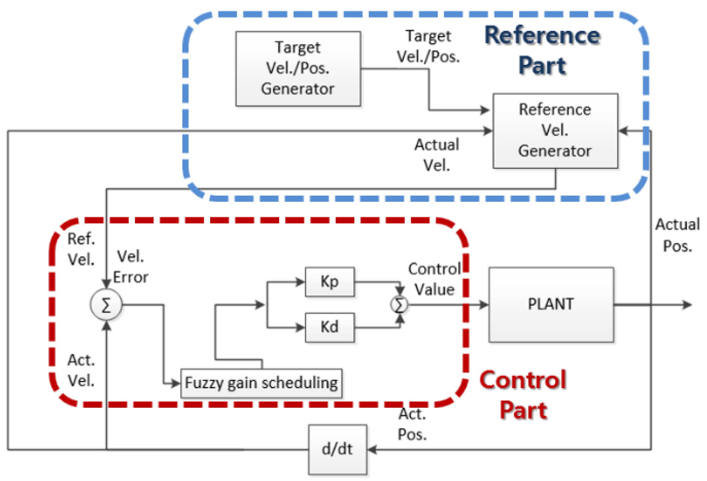
Figure 10.
PD control system.

Figure 11.
Structure of the fuzzy inference system.

Figure 12.
Membership functions of error and dot-error.

Figure 13.
Curvature tracking in the static position.

Figure 14.
Velocity profile of curvature tracking in the static position.

Figure 15.
Curvature tracking in the dynamic position.

Figure 16.
Velocity profile of curvature tracking in the dynamic position.

Figure 17.
Comparison of distances between static and dynamic curvature tracking.

Figure 18.
Overall system.

Figure 19.
Flowchart of the overall system.

Figure 20.
Moving object (Master).

Figure 21.
Mobile robot (Slave).

Figure 22.
Experimental environment.

Figure 23.
Straight line estimation.

Figure 24.
Velocity profile of the straight line estimation robot.

Figure 25.
Real-time estimated locations (a), (b). (c) (, , and ) of sound sources in the straight trajectory estimation.
Figure 25.
Real-time estimated locations (a), (b). (c) (, , and ) of sound sources in the straight trajectory estimation.


Figure 26.
The distance and angle of the straight orbit experiment.

Figure 27.
S-curved line estimation.

Figure 28.
Velocity profile of curved line estimation robot.

Figure 29.
Real-time estimated locations (a), (b). (c) (, , and ) of sound sources in curved trajectory estimation.
Figure 29.
Real-time estimated locations (a), (b). (c) (, , and ) of sound sources in curved trajectory estimation.


Figure 30.
The distance and angle of the curve orbit experiment.


Table 1.
Distance, position error, and driving time without curvature trajectory.
| Distance (m) | Error (m) | Time (m/s) | |
|---|---|---|---|
| 0.1 | 2.050 | 0.050 | 19570 |
| 0.2 | 2.303 | 0.303 | 10870 |
| 0.3 | 2.388 | 0.388 | 7670 |
| 0.4 | 2.457 | 0.457 | 5770 |
| 0.5 | 2.734 | 0.734 | 5310 |
Table 2.
Rotation radius, distance, position error, and driving time with curvature trajectory.
| Rotation (m) | Distance (m) | Error (m) | Time (m/s) | |
|---|---|---|---|---|
| 0.1 | 1.944 | 3.054 | 0.057 | 32946 |
| 0.2 | 2.174 | 3.415 | 0.171 | 18480 |
| 0.3 | 2.203 | 3.460 | 0.280 | 11962 |
| 0.4 | 2.392 | 3.757 | 0.401 | 9562 |
| 0.5 | 2.488 | 3.908 | 0.656 | 8542 |
Table 3.
The trajectory results of the root mean square error (RMSE).
| Trajectory | RMSE | |
|---|---|---|
| 0.1 | Non-curvature | 0.0025 |
| Curvature | 0.0032 | |
| 0.2 | Non-curvature | 0.0918 |
| Curvature | 0.0292 | |
| 0.3 | Non-curvature | 0.1505 |
| Curvature | 0.0784 | |
| 0.4 | Non-curvature | 0.2088 |
| Curvature | 0.1608 | |
| 0.5 | Non-curvature | 0.5388 |
| Curvature | 0.4303 |
Table 4.
Fuzzy inference for .
| NB | NM | NS | Z | PS | PM | PB | ||
|---|---|---|---|---|---|---|---|---|
| NB | B | B | B | B | B | B | B | |
| NM | S | B | B | B | B | B | S | |
| NS | S | S | B | B | B | S | S | |
| Z | S | S | S | B | S | S | S | |
| PS | S | S | B | B | B | S | S | |
| PM | S | B | B | B | B | B | S | |
| PB | B | B | B | B | B | B | B | |
Table 5.
Fuzzy inference for .
| NB | NM | NS | Z | PS | PM | PB | ||
|---|---|---|---|---|---|---|---|---|
| NB | S | S | S | S | S | S | S | |
| NM | B | B | S | S | S | B | B | |
| NS | B | B | B | S | B | B | B | |
| Z | B | B | B | B | B | B | B | |
| PS | B | B | B | S | B | B | B | |
| PM | B | B | S | S | S | B | B | |
| PB | S | S | S | S | S | S | S | |
Table 6.
Velocity profile along the curvature in the static position.
| Wheel | Left | Right | |||||
|---|---|---|---|---|---|---|---|
| Method | Velocity | Acceleration | Distance | Velocity | Acceleration | Distance | |
| Case 1 | 0.342 | 0.342 | 2.528 | 0.258 | 0.258 | 1.9 | |
Table 7.
Velocity profile of curvature in the dynamic position.
| Wheel | Left | Right | |||||
|---|---|---|---|---|---|---|---|
| Method | Velocity | Acceleration | Distance | Velocity | Acceleration | Distance | |
| Case 1 | 0.384 | 0.384 | 2.214 | 0.216 | 0.216 | 0.785 | |
| Case 2 | 0.216 | 0.216 | 0.785 | 0.384 | 0.384 | 1.413 | |
Table 8.
Results of the experiment on static and dynamic curvature trajectory.
| Curvature | Control | Distance (m) | Time (s) | Error (m) |
|---|---|---|---|---|
| Case 1 (Static) | CPID | 2.35 | 8 | 0.146 |
| CFGS-PD | 2.33 | 7.92 | 0.044 | |
| Case 2 (Dynamic) | CPID | 2.25 | 8.36 | 0.198 |
| CFGS-PD | 2.25 | 8.11 | 0.085 |
Table 9.
Results of RMSE.
| Curvature | Control | RMSE |
|---|---|---|
| Case 1 (Static) | CPID | 0.0213 |
| CFGS-PD | 0.0019 | |
| Case 2 (Dynamic) | CPID | 0.0392 |
| CFGS-PD | 0.0072 |
Table 10.
Hardware specifications of the moving object.
| List | Specification |
|---|---|
| Size (mm) | 352 (W) × 326 (L) × 320 (H) |
| Weight (kg) | 5.3 |
| Distance between wheels (mm) | 290 |
| Radius of wheel (mm) | 60 |
Table 11.
Hardware specifications of a mobile robot.
| List | Specification |
|---|---|
| Size (mm) | 280 (W) × 350 (L) × 260 (H) |
| Weight (kg) | 4.5 |
| Distance between wheels (mm) | 289 |
| Radius of wheel (mm) | 60 |
Table 12.
Components used in the experiment.
| Mobile robot | ||
| Article | Manufacturer | Goods |
| Mobile robot | PNU_IRL-LAB | PNU_IRL-LAB |
| Motor drive | NTRexLAB | NT-DC20A |
| DC motor | D&J | IG-32PGM |
| MCU | TI | LM3s8962 |
| Amplifier kit | Velleman | K2372 |
| Bluetooth module | Sena_Tech | PARANI-ESD200 |
| Battery | Anyrc | 11.1V-LiPo-Battery |
| Moving object | ||
| Article | Manufacturer | Goods |
| Moving object | NTRexLAB | NT-Commander-1 |
| MCU | TI | LM3s8962 |
| DC motor | D&J | RB-35GM |
| Battery | Anyrc | 11.1V-LiPo-Battery |
| Speaker | INKEL | INKEL 6K28G |
| Robot control board | NTRexLAB | NT-ControllerBv1 |
| Bluetooth module | Firmtech | FB100AS |
© 2019 by the author. Licensee MDPI, Basel, Switzerland. This article is an open access article distributed under the terms and conditions of the Creative Commons Attribution (CC BY) license (http://creativecommons.org/licenses/by/4.0/).
Share and Cite
MDPI and ACS Style
Han, J.-H. Tracking Control of Moving Sound Source Using Fuzzy-Gain Scheduling of PD Control. Electronics 2020, 9, 14. https://doi.org/10.3390/electronics9010014
AMA Style
Han J-H. Tracking Control of Moving Sound Source Using Fuzzy-Gain Scheduling of PD Control. Electronics. 2020; 9(1):14. https://doi.org/10.3390/electronics9010014
Chicago/Turabian StyleHan, Jong-Ho. 2020. "Tracking Control of Moving Sound Source Using Fuzzy-Gain Scheduling of PD Control" Electronics 9, no. 1: 14. https://doi.org/10.3390/electronics9010014
Note that from the first issue of 2016, this journal uses article numbers instead of page numbers. See further details here.