Semi-Autonomous Coordinate Configuration Technology of Base Stations in Indoor Positioning System Based on UWB

Abstract

In the global positioning system (GPS) denied environment, an indoor positioning system based on ultra-wide band (UWB) technology has been utilized for target location and navigation. It can provide a more accurate positioning measurement than those based on received signal strength (RSS). Although promising, it suffers from some shortcomings that base stations should be preinstalled to obtain reference coordinate information, just as navigation satellites in the GPS system. In order to improve the positioning accuracy, a large number of base stations should be preinstalled and assigned coordinates in the large-scale network. However, the coordinate setup process of the base stations is cumbersome, time consuming, and laborious. For a class of linear network topology, a semi-autonomous coordinate configuration technology of base stations is designed, which refers to three conceptions of segmentation, virtual triangle, and bidirectional calculation. It consists of two stages in every segment: Forward and backward. In the forward stage, it utilizes the manual coordinate setup method to deal with the foremost two base stations, and then the remaining base stations autonomously calculate their coordinates by building the virtual triangle train. In the backward stage, the reverse operation is performed, but the foremost two base stations of the next segment should be used as the head. In the last segment, the last two base stations should be used as the head. Integrating forward and backward data, the base stations could improve their location accuracy. It is shown that our algorithm is feasible and practical in simulation results and can dramatically reduce the system configuration time. In addition, the error and maximum base station number for one segment caused by our algorithm are discussed theoretically.

1. Introduction

The GPS signal belongs to the electromagnetic wave and cannot penetrate the reinforced concrete structure. When indoors or underground, also called GPS-deny environment, it is difficult to locate and navigate the target by GPS [1] or global navigation satellite system (GNSS) [2]. The indoor positioning system based on UWB has gradually become popular in recent years. Since UWB has the ability of an anti-multipath effect, using the methods of time of arrival (TOA) or time difference of arrival (TDOA) [3], it can provide more accurate distance measurements. Through the trilateral method, the indoor positioning system based on UWB can obtain more accurate location information than others, such as RSS [4,5,6], channel pulse response (CIR) [7], radio frequency identification (RFID) [8]. Many scholars have made comprehensive research on it. However, how to construct the indoor positioning system based on UWB and the surroundings and how to influence the system performance are the focus of their research. For instance, Ubisense in the United Kingdom (UK) has successfully established an indoor positioning system based on UWB, TDOA, and angle of arrival (AOA) [9]. Various positioning systems based on UWB have ranged in the Microsoft indoor localization competition [10]. Guido Schroeder has investigated the positioning systems based UWB and TDOA [11]. In addition, because the distance is more accurate in the line of sight (LOS) than the non-line of sight (NLOS) [12]. How to detect and identify NLOS has been paid close attention by scholars in this field, which is to mitigate the error caused by multipath effect, such as Perz Cruz has proposed that the error caused by NLOS propagation can be viewed as a random variable, and derived its probability density function (PDF) [13]. Horiba has detected the condition of NLOS by the random characteristics of the measurement error and the modified iterative minimum residual method (IMR) [14]. Liu F. has proposed a method that use complementary Kalman filters to integrate UWB and IMU data to improve positioning accuracy [15]. Gao H. has proposed a tightly coupled multi-sensor fusion algorithm to effectively reduce NLOS and multipath interference, a fuzzy calibration is introduced to adaptively adjust the dependency on the received UWB measurement [16].

Compared with RSS or CIR, UWB has the advantage that it can gain a higher positioning accuracy. However, it also has a shortcoming. In order to obtain the target location information, a large number of base stations should be pre-installed, which provide reference position information to calculate the target location. Numerous base stations should be assigned coordinates in advance. This process is rather time consuming and laborious. Most scholars still assign their base stations’ coordinates by manual operation. How to improve assignment efficiency is an important technology, but we have not found related literatures by retrieving the indoor positioning field. That is why we researched the autonomous coordinate configuration problem of base stations in this paper.

The main contribution of our paper is that, for a class of linear network topology, our algorithm can reduce the system configuration time and labor cost and guarantee the accuracy of target location within the tolerant range at the same time. Three conceptions of “segmentation”, “virtual triangle”, and “forward and backward bidirectional calibration” are introduced to our algorithm. The large- scale base stations can be divided into many little scale segments, which usually have the same number of base stations except the last segment. In every segment, only the foremost two base stations’ coordinates are set up, utilizing the common location setting method. It should be noted that the last two base stations also need to be allocated in the last segment. In the forward stage, base stations’ coordinates are calculated sequentially by virtual triangle train, the foremost two base stations of the current segment are the head. In the backward phase, the calculation process needs to be carried out in the reverse direction, and the foremost two base stations of the next segment are the head. Finally, every base station integrates the forward value and backward value to obtain more accurate coordinates.

The remaining of this paper is structured as follows. Section 2 gives an overview of the preliminary knowledge on positioning and ranging algorithm. In Section 3, the semi-autonomous configuration scheme of base stations is analyzed. In Section 4, a method is introduced to analyze the influence on positioning accuracy of our semi-autonomous configuration algorithm. At last, the simulation is performed and our algorithm’s performance is discussed in Section 5. The conclusion of this paper is given in Section 6.

2. Preliminary

The positioning technique is defined to be a set of algorithms, which is used to solve the location of the objective. It mainly includes two categories, one is based on relative range with the objective and another is based on absolute range from the reference objective (landmark, anchor, etc.). The positioning of the objective can be presented (x, y) in Cartesian or $(r,\varphi )$ in polar coordinates in two-dimension (2D). The algorithms involved in this article rely on the ranging measurements provided by the DW1000 UWB transceiver to calculate the positioning of the tag [17].

2.1. Positioning Algorithm

In this paper, trilateration is adopted, which belongs to an absolute range positioning method. One tag and three base stations exist, similar to Figure 1. Every base station knows its own coordinate. The range between the base station and tag can be measured by TOA algorithm. If all the ranges between tag and base stations are known, then the tag’s coordinate can be solved.

Given the tag 2D coordinate is $\left(x,y\right)$, $\left(x_i,y_i\right)$ are the coordinates of base stations, and $d_i$ are the ranges between base stations and tag. Then, the ranges can be defined as Equation (1)

$$d_i^2={(x-x_i)}^2+{(y-y_i)}^2=x^2-2x_{i}x+x_i{}^2+y^2-2y_{i}y+y_i{}^2$$

(1)

Nonlinear terms $x^2$ and $y^2$ exist in Equation (1), which can be eliminated by subtraction operation between $d_i^2$ and $d_N^2$.

$$d_i^2-d_N^2=-2x(x_i-x_N)+x_i^2-x_N^2-2y(y_i-y_N)+y_i^2-y_N^2$$

(2)

When n base stations exist in a network, a matrix representation form $b=A\left[\begin{array}{c}x\\ y\end{array}\right]$ can be presented,

$$b=\left[\begin{array}{c}{d}_1^2-d_N^2-(x_1^2+y_1^2)+(x_N^2+y_N^2)\\ d_2^2-d_N^2-(x_2^2+y_2^2)+(x_N^2+y_N^2)\\ ⋮\\ d_{N-1}^2-d_N^2-(x_{N-1}^2+y_{N-1}^2)+(x_N^2+y_N^2)\end{array}\right]$$

(3)

$$A=-2\left[\begin{array}{cc}\begin{array}{c}{x}_1-x_N\\ x_2-x_N\end{array}& \begin{array}{c}{y}_1-y_N\\ y_2-y_N\end{array}\\ \begin{array}{c}⋮\\ x_{N-1}-x_N\end{array}& \begin{array}{c}⋮\\ y_{N-1}-y_N\end{array}\end{array}\right]$$

(4)

Therefore, the tag coordinate can be transformed into the matrix solution.

2.2. Ranging Algorithm

The range between base station and the tag can be measured by the TOA algorithm. The method usually relies on the exchange of signal messages between the two nodes [18]. In order to degrade the effect of the conventional two way ranging (TWR) [19]. The range can be calculated through the symmetric double-sided two-way ranging (SDS-TWR) algorithm [20], depicted in Figure 2. Device A sends a POLL packet and transmission time is T₁. Device B turns on the receiver in advance, and receives the POLL packet, recording time T₂. Device B sends the response packet at T₃ (T₃ = T₂ + T_reply1). Device A receives the response packet and records the time T₄. Device A sends a final packet at T₅ (T₅ = T₄ + T_reply2). Device B receives the final packet and records the time T₆.

The estimation value of TOA is ${\widehat{T}}_{prop}$, and can be calculated using Equation (5):

$${\widehat{T}}_{prop}=\frac{T_{round1}\times T_{round2}-T_{reply1}\times T_{reply2}}{T_{round1}+T_{round2}+T_{reply1}+T_{reply2}}$$

(5)

When the TOA has been known, the range can be calculated by multiplying light speed. The accuracy of ranging makes a great influence on positioning accuracy. Therefore, there are many algorithms to improve ranging accuracy, such as the enhanced asymmetric DS-TWR [21].

3. Semi-Autonomous Configuration Scheme of Base Stations

Considering the environment of a mine or tunnel, base stations are deployed at a certain interval on both sides of the mine or tunnel. It is a long linear topology network and can be used for target location and tracking. As shown in Figure 3, the base stations are represented as BS_i (i = 1, 2, 3 …).

As mentioned in the preliminary sections, the coordinates of the base stations should be known first. In convention scheme, such process is completed manually, every base station should be measured and calibrated by the instrument. It is time-consuming and laborious, even inconvenient in the field of the mine or tunnel. In the paper, we present a semi-autonomous coordinate configuration strategy based on “segmentation”, “virtual triangle”, and “forward-backward bidirectional calculation” to assign coordinates for base stations.

3.1. Semi-Autonomous Coordinate Configuration Strategy

The so-called semi-autonomous configuration means that most of the base stations can calculate their coordinates by program. There are only two types of base stations in the network, one is needed to assign coordinates by convention operation, and another is needed to calculate by our algorithm. Due to the multipath effect and ambient environment, there exists an error in the calculating process. We have taken some measures to reduce the error and improve accuracy. The first measure is to divide the large-scale network into many segments to reduce cumulative error. The second measure is to calculate bidirectional to reduce error. It mainly consists of two stages: Forward and backward. The foremost two base stations should be assigned coordinates in every segment. It should be noted that, in the last segment, all the foremost two base stations and the last two base stations should be assigned coordinates. The other coordinates would be calculated by semi-autonomous algorithm. In the forward stage, the foremost two base stations of the current segment are the head, the other coordinates would be calculated by virtual triangle train. In the backward stage, the reverse operation process works, but the foremost two base stations of the next segment are as head. In the last segment, it should be adopted that the last two base stations to be its head. That is the main difference in the two stages. Integrating forward and backward data, the base stations could promote their location accuracy. How to build virtual triangles will be discussed in the next section.

In Figure 4, all the base stations are fixed on both sides of the tunnel. As above-mentioned, this segment’s foremost two base stations’ coordinates are first assigned. Their absolute position information usually are obtained through a series of physical methods, such as laser measurement or high-precision GPS instrument. For such network topology, semi-autonomous coordinate calculation of base stations begins with building a sequential virtual triangle.

3.2. Semi-Autonomous Configuration Process and Algorithm

In a large-scale network, the semi-autonomous coordinate configuration algorithm will increase the cumulative error to lead to a positioning accuracy out of tolerance. Therefore, the large-scale network should be divided into a reasonable scale segment firstly. Our algorithm is implemented in every segment, which improves the accuracy of the positioning.

Therefore, taking one segment as an example, our algorithm is composed of four steps. Firstly, all the foremost two base stations of every segment should be assigned as convention. They will be used as the reference for the semi-autonomous configuration. Secondly, the virtual triangle train would be constructed and un-calibrated base stations’ coordinates would be calculated. Thirdly, the backward calibration procedure would be carried out. It has the same operation as the second step in the forward procedure, but using different reference base stations. Lastly, every un-calibrated base station’s coordinate would be calculated by averaging the coordination value from the forward and backward procedure.

Real time ranging data acquisition between the base stations is the premise of building a virtual triangle. Through measuring propagation time $t_i$ and multiplying by the propagation speed of radio wave $c$, the range $l_i$ can be achieved as Equation (6)

$$l_i=t_i\times c/2$$

(6)

It is a very important step to choose out the un-calibration base station from the adjacent candidate base stations to build a virtual triangle. Here, the “proximity principle” is adopted. As shown in Figure 5, one base station should be selected to construct a virtual triangle, combing with the pre-calibration base stations BS₁ and BS₂. BS₃ and BS₄ are the candidates. The ranges between BS₁ and BS₃, BS₁ and BS₄, BS₂ and BS₃, and BS₂ and BS₄ are $l_2$, $l_6$, $l_3$ and $l_4$, respectively. Based on the “proximity principle”, if $l_2+l_3<l_4+l_6$, the base station BS₃ is selected. If $l_2+l_3=l_4+l_6$, then the bottom right base station BS₃ is preferred.

Once the virtual triangle is determined, the un-calibrated base station coordinate estimation is transformed into a problem on how to calculate the vertex coordinate of the virtual triangle. The vertex coordinate can be solved by the following algorithm in Section 3.3.

3.3. Un-Calibrated Base Station Coordinate Estimation Algorithm of Virtual Triangle

Suppose a virtual triangle has been constructed, which has three vertices of BS₁ (x1, y1), BS₂ (x2, y2), and BS₃. The coordinate of BS₃ should be estimated. The procedure on how to calculate the unknown coordinates of the vertex is as follows:

(1)

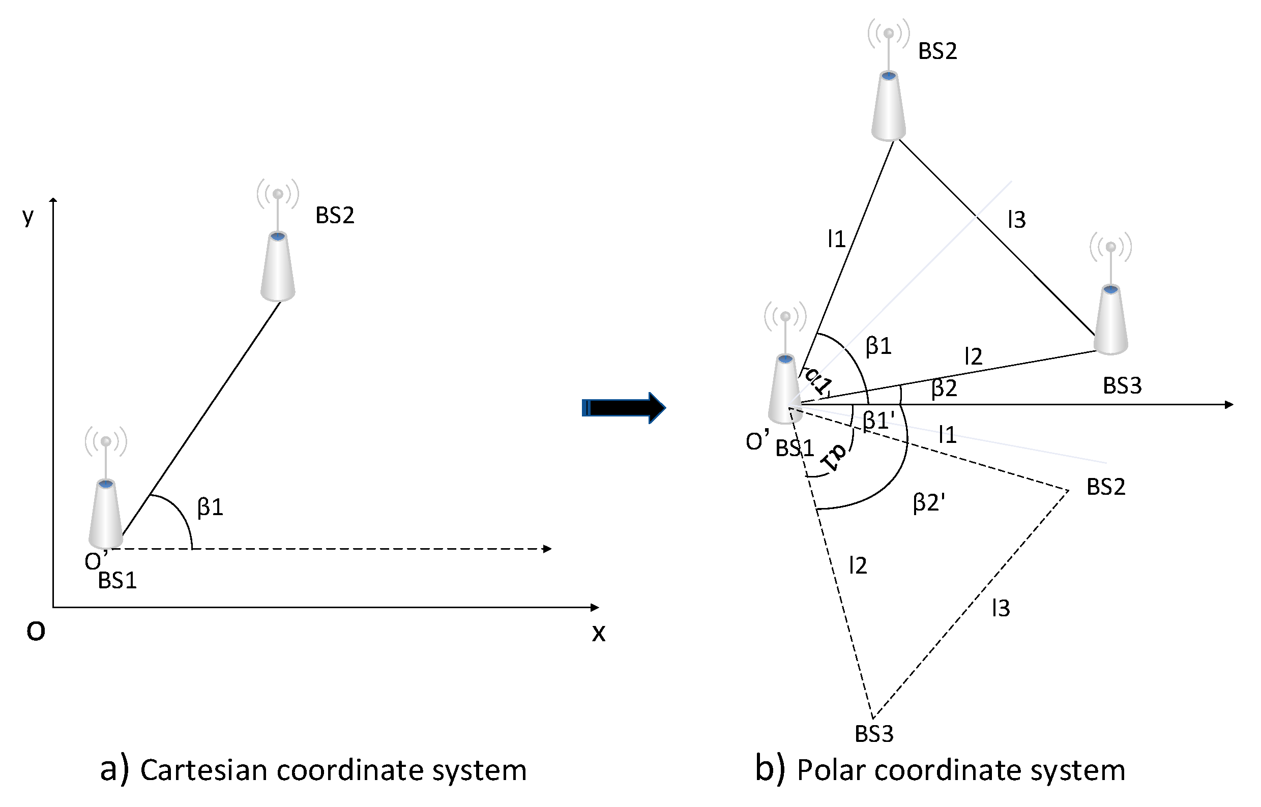
Suppose that the ranges between BS₁ and BS₂, BS₁ and BS₃, BS₂ and BS₃ are set to be $l_1$, $l_2$, and $l_3$, respectively. They can be measured and regarded as known quantity. In accordance with the cosine theorem, angle ${\alpha }_1$ starting from the edge of BS₁ and BS₃ to the edge of BS₁ and BS₂ is calculated by Equation (7). For the convenience of calculation, some intermediate calculation process needs to be transformed to the Cartesian coordinate system, because the angle ${\beta }_1$ starting from the x-axis or horizontal ray to the edge of BS₁ and BS₂ are the same degree in the two coordinate systems, as shown in Figure 6. In the Cartesian coordinate system, angle ${\beta }_1$ is easily calculated by Equation (8).

$${\alpha }_1=co{s}^{-1}(\frac{l_1^2+l_2^2-l_3^2}{2l_1{l}_2})$$

(7)

$${\beta }_1={\tan }^{-1}\frac{y_2-y_1}{x_2-x_1}, {\beta }_1\in (-90°,90°)$$

(8)

(2)

As shown in Figure 6b, ${\beta }_2$ or ${\beta }_2^{\prime }$ is the angle starting from the edge of BS₁ and BS₃ to the horizontal ray from BS₁, in the polar coordinate system. In the application field, there are two deployment scenarios, as shown in Figure 7. One is that there is only a straight-line arrangement, the other is that there is a turning at the tail. In transfer procedure of the virtual triangle, the solid line triangle is illuminated for the coordinate estimation transfer process for the first case, and the dotted line triangle is illuminated for another. For simplicity, in the text, the first case is studied and discussed. Another case is the same, just one more judgement step is added. Therefore, in our algorithm, only the azimuth ${\beta }_2$ is calculated by

$${\beta }_2={\beta }_1-{\alpha }_1$$

(9)

(3)

Transform the polar coordinate system to the Cartesian coordinate system and calculate the coordinates of base station BS₃ by Equations (10) and (11), as depicted in Figure 8.

$$x_3=x_1+l_2\cos {\beta }_2$$

(10)

$$y_3=y_1+l_2\sin {\beta }_2$$

(11)

(4)

Through the above steps, we can get all vertex coordinates of the virtual triangle. As shown in Figure 9, they are the base stations BS₁, BS₂, and BS₃. Since the coordinate of BS₃ has been calculated, it can be viewed as a new pre-calibrated base station and would form a new virtual triangle with the original base station BS₂ and the next unknown base station BS₄. Then, the virtual triangle procedure transfers to the next. The coordinate of BS₄ needs to be calculated. That is to say, such procedure would repeat until all the base stations’ coordinates are obtained in one segment.

(5)

In addition, a backward operation methodology is adopted and applied to our algorithm. As shown in Figure 10, the pre-calibrated base stations in the next segment can serve as the start of the backward procedure for the previous segment. The procedure is just the same as the aforementioned steps 1 to 4 in the forward. After that, for all the base stations, we can get two sets of values, forward and backward. In our algorithm, the base station coordinate can be determined by the average to improve accuracy.

(6)

Thus far, one segment can be completed. Such procedure should be iterated until all segments are completed. Please note that the last segment is different from the other previous segments, because there are four base stations needed to be pre-calibrated, the foremost two and the last two base stations. The procedure also can be described as Algorithm A1 in Appendix A.

4. Method for Analyzing Semi-Autonomous Configuration Technology Influence on Positioning Accuracy

During the UWB signal propagation and procession, errors will be introduced to cause ranging error. The positioning buildup of error will increase along with the virtual triangle transfer. The accuracy based on UWB is expected to be a centimeter order of magnitude. Once the buildup of error is out of such range, the semi-autonomous configuration method would be considered a failure. Therefore, the method for analyzing semi-autonomous configuration influence on positioning accuracy would be presented in this section. The location estimation process of the tag is shown in Figure 11.

According to the application, the error should be controlled to minimum to degrade its influence on the positioning accuracy. Considering that buildup of error would increase along with the virtual triangle transfer, the quantity of base stations arranged in one segment should be discussed. Assume that N base stations are arranged in the segment, the $i$-th BS position is $\left(x_i,y_i\right)$. The coordinates of the tag or target to be located is (x, y). The range from target is $l_i$. An equation can be established based on the measured TOA ${\tau }_i$.

$$\begin{gathered} l_i^2={\left[x-\left(x_i+s_i\right)\right]}^2+{\left[y-\left(y_i+s_i\right)\right]}^2=P_i-2x\left(x_i+s_i\right)-2y\left(x_i+s_i\right)+L={\left(c{\tau }_i\right)}^2 i \\ =1,2\dots ,N \end{gathered}$$

(12)

where $P_i=x_i^2+y_i^2$, $L=x^2+y^2$, and c is the speed of radio wave propagation. $s_i$ is the base station configuration error.

Let $z_a=\left[z_p^T,L\right]$ be an unknown vector, $z_p={\left[x,y\right]}^T$. From Equation (12), a linear equation with $z_a$ as a variable can be established.

$$h=G_a{z}_a$$

(13)

where $h=\left[\begin{array}{c}{l}_1^2-P_1\\ l_2^2-P_2\\ \begin{array}{c}⋮\\ l_N^2-P_N\end{array}\end{array}\right], G_a=\left[\begin{array}{c}\begin{array}{ccc}-2\left(x_1+s_1\right)& -2\left(y_1+s_1\right)& 1\end{array}\\ \begin{array}{ccc}-2\left(x_2+s_2\right)& -2\left(y_2+s_2\right)& 1\end{array}\\ \begin{array}{c}\begin{array}{ccc}⋮& ⋮& ⋮\end{array}\\ \begin{array}{ccc}-2\left(x_N+s_N\right)& -2\left(y_N+s_N\right)& 1\end{array}\end{array}\end{array}\right]$.

Then, the error vector corresponding to the target estimated position is

$$\psi =h-G_a{z}_a^0$$

(14)

where $z_a^0$ is the $z_a$ value corresponding to the actual position of the target. The weighted least squares (WLS) method [22] can be used and the covariance matrix of the error $\psi$ can be replaced by the covariance matrix Q of the TOA, which can be obtained

$$z_a=\underset{Q }{\mathrm{argmin}}\left\{{\left(h-G_a{z}_a\right)}^T{Q}^{-1}\left(h-G_a{z}_a\right)\right\}={\left(G_a^T{Q}^{-1}{G}_a\right)}^{-1}\left(G_a^T{Q}^{-1}h\right)$$

(15)

The coordinate of (x, y) in $z_a$ is the approximate estimated position of the target. Assuming that the TOA measurements are independent of each other, the Q matrix in Equation (15) is a diagonal matrix. $\mathsf{\sigma }$ is the ranging error.

$$Q=diag\left({\sigma }_1^2,{\sigma }_2^2,\dots ,{\sigma }_N^2\right)$$

(16)

In Equation (14), since L in $z_a$ is a quantity actually related to (x, y), using approximation of Q matrix to replace the covariance matrix of the error vector $\psi$ will lead to error. In order to obtain a more accurate estimated position, a similar processing method can be used, just as the Chan algorithm. When the error of TOA is small, the error vector corresponding to the N quantiles of TOA measurements is

$$\psi =2B\mu +\mu \cdot \mu \approx 2B\mu , B=diag\left\{l_1^0,l_2^0,\dots ,l_N^0,\right\}$$

(17)

where the sign “$·$” represents the Schur product, $l_i^0$ is the actual range between the target and $i$-th base station, and the $\mu$ is the TOA measurement error, which approximately follows a normal distribution.

Using TOA measurements to build the covariance matrix of error vector $\psi$ in Equation (14).

$$\psi =E\left[\psi {\psi }^T\right]=4BQB$$

(18)

where Q is the covariance matrix of the TOA.

In order to obtain the B matrix, the measured $l_1$ can be substituted for $l_i^0$, and the first WLS estimated value of $z_a$ is

$$z_a={\left(G_a^T{\psi }^{-1}{G}_a\right)}^{-1}\left(G_a^T{\psi }^{-1}h\right)$$

(19)

Using the $z_a$ value, we can get the new matrix of B. Using such a process, an improved estimated position can be obtained.

$${\epsilon }_x=x_i^a-x$$

(20)

$${\epsilon }_y=y_i^a-y$$

(21)

$$l_i^{\prime }=\sqrt{{({\epsilon }_x{}^i)}^2+{({\epsilon }_y{}^i)}^2}$$

(22)

where $\left(x_i^a,y_i^a\right)$ is the estimated coordinate, $({\epsilon }_x,{\epsilon }_y)$ is the error of positioning, $l_i^{\prime }$ is the error of the range between the tag and base station.

The range of the error can be calculated by the root mean square (RMS).

$${\epsilon }_l(RMS)=\sqrt{{\displaystyle \sum _{i=1}^{n-2}{(l_i{}^{\prime })}^2}}$$

(23)

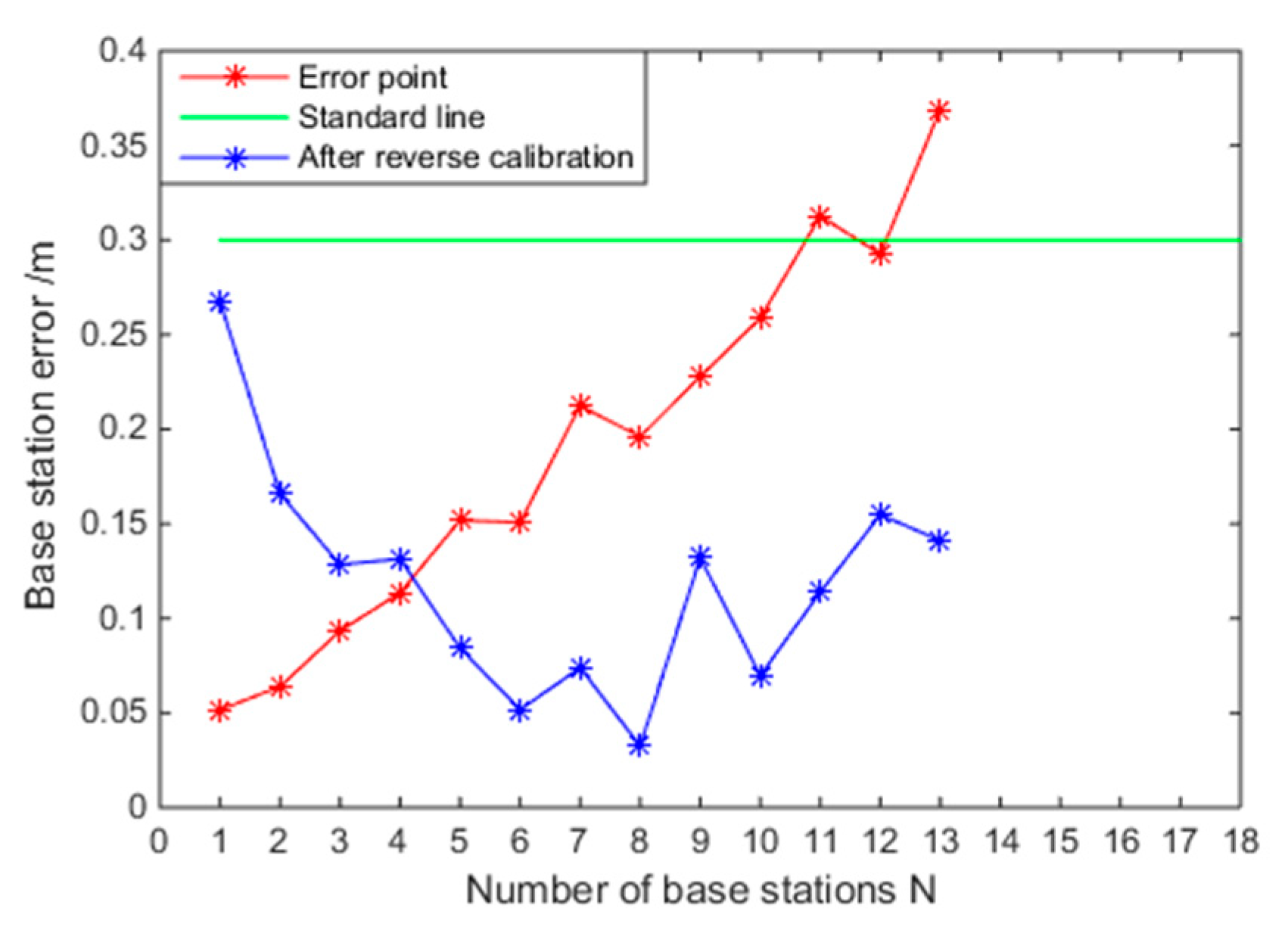
5. Simulation and Performance Discussion of Semi-Autonomous Configuration Algorithm of Base Stations

We have simulated our semi-autonomous configuration algorithm to analyze and discuss its performance. The network deployment is just as shown in Figure 12, but only one segment is adopted to illustrate. The pre-calibrated base stations are placed at (0, 0) and (15, 25.982), the others are placed evenly on both sides of the channel with an interval about 30 m. All the base stations can communicate with wireless communication mutually. The noise generated during signal transmission is replaced by Gaussian white noise N (0, 0.1).

Compared with the manual operation configuration, the semi-autonomous configuration technology studied in this paper has greatly reduced the initial complexity and cost. Given that N base stations need to be configured in the scenario, N manual operations should be performed. However, if the whole network is divided into M segments, and using our algorithm, the number of operations is deduced to 2 × M + 2. Therefore, the cost and time consumed by our semi-autonomous configuration algorithm to manual operation is

$$A_N=\frac{2\times M+2}{N}\left(M\approx \raisebox{1ex}{$N$}\!\left/ \!\raisebox{-1ex}{$14$}\right.\right)$$

(24)

Therefore, our semi-autonomous coordinate configuration technology of base stations almost saves 70% of the cost compared to manual configuration.

Due to the influence of multi-path effect, UWB signals propagation would cause a ranging error. As semi-autonomous process is adopted, the error will increase when the virtual triangle transfer in sequence. The simulation results are shown in Figure 13 and Figure 14. The blue circle and the red star represent the position of the actual calibration result and the standard base station, respectively. The blue line error increases with the increasing distance of the base stations, which indicates that the error of the base stations increases as the number of base station arrangements increases.

As described, we have adopted the segmentation method to ensure the accuracy of semi-autonomous configuration of the base stations. Additionally, how many base stations should be arranged to one segment is considered. Considering the positioning accuracy of UWB technology about the magnitude of centimeter level, our exception is to control the accuracy within 30 cm. Through simulating our semi-autonomous algorithm, when just forward calculation operation is performed, the errors of the 14th and 15th base stations have fluctuated around 0.3 m in Figure 15. This means that the maximum number of base stations arranged in one segment is 14.

In our semi-autonomous algorithm, the backward operation is also introduced. The 15th and 16th base station would be used as pre-calibrated base stations to calculate base stations’ coordinates of the previous segment. Through integrating forward and backward data, the average is obtained, and the base stations could promote their location accuracy. The simulation result is shown in Figure 16. As shown, the base stations’ error of the semi-autonomous calculation after backward and forward operation is reduced. The accuracy of base stations has been reduced from 3% to 1.5%.

Now, we know that the semi-autonomous configuration process causes deviations. In order to analyze the impact to positioning accuracy, we have utilized the Monte Carlo method and performed 50 tests to simulate the range error of the tag. Figure 17 and Figure 18 are a comparison of influences on positioning errors by manual and semi-autonomous methods to configure base stations. As shown in the two Figures, the errors caused by our semi-autonomous algorithm is slightly larger than the conventional on-site manual operation method. However, the positioning error fluctuates within the range of −0.1 to 0.2 m by our algorithm. It has little impact on scenarios such as general tunnels and mines and meets our design exception. That is to say, our semi-autonomous coordinate configuration technology of base stations is feasible and practical.

6. Conclusions

For the shortcoming of the indoor positioning system based on UWB that a great number of base stations should be preinstalled to obtain reference location information, a lot of onsite manual operations should be performed to set up their coordinate parameter in a large-scale network system. However, the coordinate setup process of the base stations is cumbersome, time-consuming and laborious. For a class of linear network topology, a semi-autonomous coordinate configuration technology of base stations is proposed in this paper. Our main contribution is to make the setup process semi-autonomous by referring to three conceptions of segmentation, virtual triangle, and bidirectional calculation. Our algorithm can save a lot of time and labor and does not degrade positioning accuracy. We also discuss the number of base stations assigned in one segment and make simulation to verify the algorithm’s performance. The simulation results show that the method is feasible and practical. In the future, we will discuss the non-linear network topology.

References

1. Kian Meng, T.; Choi Look, L. GPS and UWB Integration for indoor positioning. In Proceedings of the 6th International Conference on Information, Communications & Signal Processing, Singapore, 10–13 December 2007; pp. 1–5. [Google Scholar]
2. Kolakowski, J.; Consoli, A.; Djaja-Josko, V.; Ayadi, J.; Morrigia, L.; Piazza, F. UWB localization in EIGER indoor/outdoor positioning system. In Proceedings of the IEEE 8th International Conference on Intelligent Data Acquisition and Advanced Computing Systems: Technology and Applications (IDAACS), Warsaw, Poland, 24–26 September 2015; pp. 845–849. [Google Scholar]
3. Goswami, S. Indoor Location Technologies; Springer: New York, NY, USA, 2013. [Google Scholar]
4. Singh, G.; Sahu, S. Review on “Really Simple Syndication (RSS) Technology Tools”. In Proceedings of the IEEE International Conference on Computational Intelligence & Communication Technology, Ghaziabad, India, 13–14 February 2015; pp. 757–761. [Google Scholar]
5. Zanella, A.; Bardella, A. RSS-Based Ranging by Multichannel RSS Averaging. IEEE Wirel. Commun. Lett. 2014, 3, 10–13. [Google Scholar] [CrossRef]
6. Shi, L.-F.; Wang, Y.; Liu, G.; Chen, S.; Zhao, Y.; Shi, Y.-F. A Fusion Algorithm of Indoor Positioning Based on PDR and RSS Fingerprint. IEEE Sens. J. 2018, 18, 9691–9698. [Google Scholar] [CrossRef]
7. Ni, T.; Su, S.; Cheng, A.; Lu, S.; Su, T.; Chang, C.C.; Fang, D.; Tai, J. “Challenge of 12” CIS CSP development, explore via finite element method. In Proceedings of the 2015 10th International Microsystems, Packaging, Assembly and Circuits Technology Conference (IMPACT), Taipei, Taiwan, 21–23 October 2015; pp. 281–284. [Google Scholar]
8. Gharat, V.; Colin, E.; Baudoin, G.; Richard, D. Indoor performance analysis of lf-rfid based positioning system: Comparison with uhf-rfid and uwb. In Proceedings of the IEEE Indoor Positioning and Indoor Navigation Conference (IPIN 2017), Sapporo, Japan, 18–21 September 2017; pp. 1–8. [Google Scholar]
9. Dardari, D.; Win, M. Threshold-based time-of-arrival estimators in UWB dense multipath channels. In Proceedings of the 2006 IEEE International Conference on Communications, Istanbul, Turkey, 11–15 June 2006; pp. 4723–4728. [Google Scholar]
10. Lymberopoulos, D.; Liu, J. The microsoft indoor localization competition: Experiences and lessons learned. IEEE Signal Process. Mag. 2017, 34, 125–140. [Google Scholar] [CrossRef]
11. Schroeer, G. A Real-Time UWB Multi-Channel Indoor Positioning System for Industrial Scenarios. In Proceedings of the International Conference on Indoor Positioning and Indoor Navigation (IPIN), Nantes, France, 24–27 September 2018; pp. 1–5. [Google Scholar]
12. Otim, T.; Díez, L.E.; Bahillo, A.; Iturri, P.L.; Falcone, F. Effects of the Body Wearable Sensor Position on the UWB Localization Accuracy. Electronics 2019, 8, 1351. [Google Scholar] [CrossRef] [Green Version]
13. Perez-Cruz, F.; Lin, C.-K.; Huang, H. BLADE: A Universal Blind Learning Algorithm for ToA Localization in NLOS Channels. In Proceedings of the 2016 IEEE Globecom Workshops (GC Wkshps), Washington, DC, USA, 4–8 December 2016; pp. 1–7. [Google Scholar]
14. Horiba, M.; Okamoto, E.; Shinohara, T.; Matsumura, K. An improved NLOS detection scheme using stochastic characteristics for indoor localization. In Proceedings of the 2015 International Conference on Information Networking (ICOIN), Siem Reap, Cambodia, 12–14 January 2015; pp. 478–482. [Google Scholar]
15. Liu, F.; Li, X.; Wang, J.; Zhang, J. An Adaptive UWB/MEMS-IMU Complementary Kalman Filter for Indoor Location in NLOS Environment. Remote Sens. 2019, 11, 2628. [Google Scholar] [CrossRef] [Green Version]
16. Gao, H.; Li, X. Tightly-Coupled Vehicle Positioning Method at Intersections Aided by UWB. Sensors 2019, 19, 2867. [Google Scholar] [CrossRef] [PubMed] [Green Version]
17. Ferreira, A.G.; Fernandes, D.; Catarino, A.P.; Monteiro, J.L. Performance Analysis of ToA-Based Positioning Algorithms for Static and Dynamic Targets with Low Ranging Measurements. Sensors 2017, 17, 1915. [Google Scholar] [CrossRef] [PubMed]
18. Shah, S.; Demeechai, T. Multiple Simultaneous Ranging in IR-UWB Networks. Sensors 2019, 19, 5415. [Google Scholar] [CrossRef] [PubMed] [Green Version]
19. Barua, B.; Kandil, N.; Hakem, N. On performance study of TWR UWB ranging in underground mine. In Proceedings of the 6th International Conference on Digital Information, Networking, and Wireless Communications, Beirut, Lebanon, 25–27 April 2018; pp. 28–31. [Google Scholar]
20. Wang, X.; Wang, Z.; Dea, B. A TOA based location algorithm reducing the error due to non-line-of-sight (NOLS) propagation. IEEE Trans. Veh. Technol. 2003, 52, 112–116. [Google Scholar] [CrossRef]
21. Kwak, M.; Chong, J. A new double two-way ranging algorithm for ranging system. In Proceedings of the IEEE International Conference on Network Infrastructure and Digital Content, Beijing, China, 24–26 September 2010; pp. 470–473. [Google Scholar]
22. Wang, G.; Cai, S.; Li, Y.; Ansari, N. A Bias-Reduced Nonlinear WLS Method for TDOA/FDOA-Based Source Localization. IEEE Trans. Veh. Technol. 2016, 65, 8603–8615. [Google Scholar] [CrossRef]
Figure 1. Principle of trilateration based on TOA (time of arrival) method.
Electronics 09 00033 g001
Figure 2. Principle of double-sided two-way ranging with three messages. Where T r o u n d 1 = T 4 T 1 , T r o u n d 2 = T 6 T 3 , T r e p l y 1 = T 3 T 2 , and T r e p l y 2 = T 5 T 4 .
Electronics 09 00033 g002
Figure 3. Linear network topology of base stations in the tunnel or mine.
Electronics 09 00033 g003
Figure 4. Diagram of building virtual triangles.
Electronics 09 00033 g004
Figure 5. Proximity principle to select neighbor base station.
Electronics 09 00033 g005
Figure 6. Coordinate system transformation process.
Electronics 09 00033 g006
Figure 7. Typical deployment scenarios of base stations in field.
Electronics 09 00033 g007
Figure 8. Coordinate transform to estimate virtual triangle unknown vertex.
Electronics 09 00033 g008
Figure 9. Virtual triangle transfer process in one segment.
Electronics 09 00033 g009
Figure 10. Presentation of backward calibration process.
Electronics 09 00033 g010
Figure 11. Location estimation process of the tag.
Electronics 09 00033 g011
Figure 12. Coordinate system for our semi-autonomous configuration technology.
Electronics 09 00033 g012
Figure 13. Error variation chart as base station location changes (one side).
Electronics 09 00033 g013
Figure 14. Error variation chart as base station location changes (another side).
Electronics 09 00033 g014
Figure 15. Maximum number of base stations when positioning error is over the exception value.
Electronics 09 00033 g015
Figure 16. Comparison chart after bidirection calibration and only forward calibration.
Electronics 09 00033 g016
Figure 17. Target positioning error on x axis.
Electronics 09 00033 g017
Figure 18. Target positioning error on y axis.
Electronics 09 00033 g018