LOCOFloat: A Low-Cost Floating-Point Format for FPGAs.: Application to HIL Simulators

Abstract

One of the main decisions when making a digital design is which arithmetic is going to be used. The arithmetic determines the hardware resources needed and the latency of every operation. This is especially important in real-time applications like HIL (Hardware-in-the-loop), where a real-time simulation of a plant—power converter, mechanical system, or any other complex system—is accomplished. While a fixed-point gets optimal implementations, using considerably fewer resources and allowing smaller simulation steps, its use is very restricted to very specific applications, as its design effort is quite high. On the other side, IEEE-754 floating-point may have resolution problems in case of the 32-bit version, and excessive hardware usage in case of the 64-bit version. This paper presents LOCOFloat, a low-cost floating-point format designed for FPGA applications. Its key features are soft normalization of the results, using significand and exponent fields in two’s complement. This paper shows the implementation of addition, subtraction and multiplication of the proposed format. Both IEEE-754 versions and LOCOFloat are compared in this paper, implementing a HIL model of a buck converter. Although the application example is a HIL simulator, other applications could take benefit from the proposed format. Results show that LOCOFloat is as accurate as 64-bit floating-point, while reducing the use of DSPs blocks by $84\%$.

1. Introduction

Most FPGA (Field Programmable Gate Array) designs must meet some area or speed constraints. Indeed, usually a trade-off between both requirements has to be reached. This compromise appears especially in real-time applications, such as digital control, live audio and video processing and HIL (Hardware-in-the-loop) applications. Apart from the algorithm complexity, the arithmetic plays a leading role, because its complexity determines the latency of every mathematical operation and the required area.

The arithmetics can be divided into two big groups: fixed-point and floating-point. Fixed-point provides an optimal approach in FPGAs, minimizing area and maximizing speed, so many examples in the literature use it [1,2,3,4,5,6]. However, floating-point provides a bigger dynamic range, adapting the point location as it is required. Besides, for the designer it is easier to use floating-point, because it is not required to think in advance the numeric range required by the application. Another important reason to prefer floating-point over fixed-point is that the former optimizes its resolution using a couple of fields that defines the mantissa and exponent along with normalization, based on scientific notation. However, fixed-point has a fixed resolution defined at design time. Anyway, the total variable width should be taken into account to prevent resolution issues in both cases.

Therefore, floating-point is the first choice when area and time constraints can be met, so many proposals use it [7,8,9]. As the overhead of floating-point is high, several algorithms to implement floating-point operators in an optimized way—in area or latency—can be found in the literature, for example [10,11]. In [10] an optimized multiplier architecture to be implemented in Xilinx FPGAs is presented, and in [11] a quadruple precision divider architecture is shown. While those optimization algorithms improve the default floating-point synthesis results, they are ad-hoc operators that have to be integrated in the desired design, including the code, or instantiating external IP (Intellectual Property) cores. Therefore, it is not a straightforward approach.

With the aim of reducing the floating-point latency, in the recent years, HFP (Hardened Floating-Point) cores have been included in some FPGA families like in Intel Arria 10 [12], and some works already use them [13,14]. The main advantage of HFP is that they are implemented in silicon, offering optimal latency results, but it is a considerably more expensive approach and the number of HFP cores is limited. When HFP cores are not available, which is at the moment, the common case, floating-point is normally implemented using the standard HDL libraries. Until some years ago, standard VHDL float package—based on the floating-point standard IEEE-754—included in the standard VHDL-2008 [15] could not be synthesized in many synthesizers. Apart from that, their implementation results were very poor, creating slow and big designs [16]. Recently, synthesis tools have made optimized implementations of floating-point, reducing the speed gap between both arithmetics. Where fixed-point arithmetic still gets much better results even now is regarding hardware usage [17]. Therefore, the resource usage of IEEE-754 floating-point is still a bottleneck for complex algorithms.

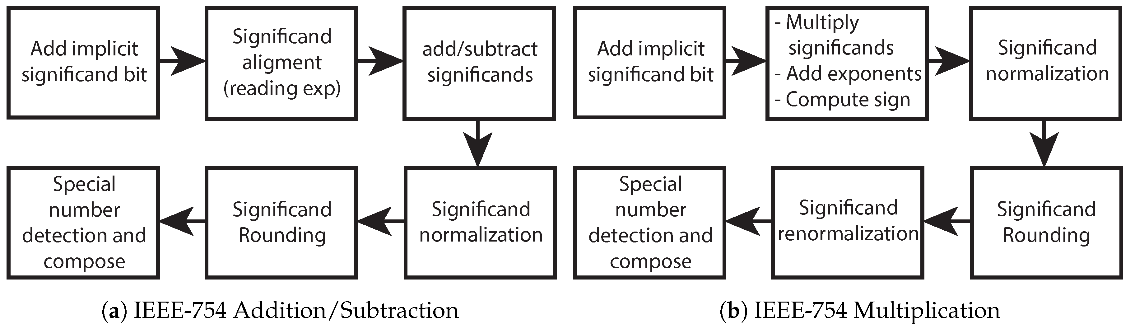
As can be seen, there is a trade-off between speed, area and design effort, so the requirements of the application determine the choice of the arithmetic. This paper presents LOCOFloat (Low-Cost Floating-point) format, which implements a floating-point arithmetic specially designed for FPGA implementation. Avoiding the overhead of the IEEE-754 floating-point standard that implements a lot of operators, with many special cases checking (e.g., NAN: Not a Number checks), rounding and normalization, the proposed format requires much fewer resources, while keeping high numerical accuracy.

In this paper, LOCOFloat is applied to an HIL simulator, but it can be used in many other applications. HIL simulators allow for testing, in real-time, the controller along with a mathematical model of the plant, instead of using the real power converter, meeting the requirements of safety, speed, and reliability. The growth of HIL is summarized by Vijay et al. [18], who presented an extensive review of simulation alternatives for microgrids, showing the consolidated use of HIL in power electronics. Anyway, HIL is applied to many fields inside power electronics, with examples of Packed U-Cell Converters (PUC) [19], resonant LLC models [20], battery management [21], renewable energy plants [18], modular multilevel converters [22], simple power converters [23], etc.

Therefore, this paper presents the details of LOCOFloat format. Its key features are the use of 50-bit mantissa in two’s complement and soft-normalization. This paper only shows the implementation details of addition, subtraction and multiplication. Besides, in the proposed model, NaN and other special cases are not needed, as only the aforementioned operations are implemented, and the inputs are not expected to be NaN. This simplification provides better area and time results.

This paper also presents a thorough comparison with the standard 32-bit and 64-bit floating point. For the comparison, a real-time mathematical model of a buck converter with electrical losses is used, showing the hardware usage and accuracy results of all the arithmetics.

The rest of the article is organized as follows: Section 2 shows how to model a power converter using Explicit Euler method. Section 3 details the available standard arithmetics that are available for FPGAs. Section 4 shows the proposed arithmetic format. The experimental results are shown in Section 5 and, finally, the conclusions are shown in Section 6.

2. Model of the Power Converter

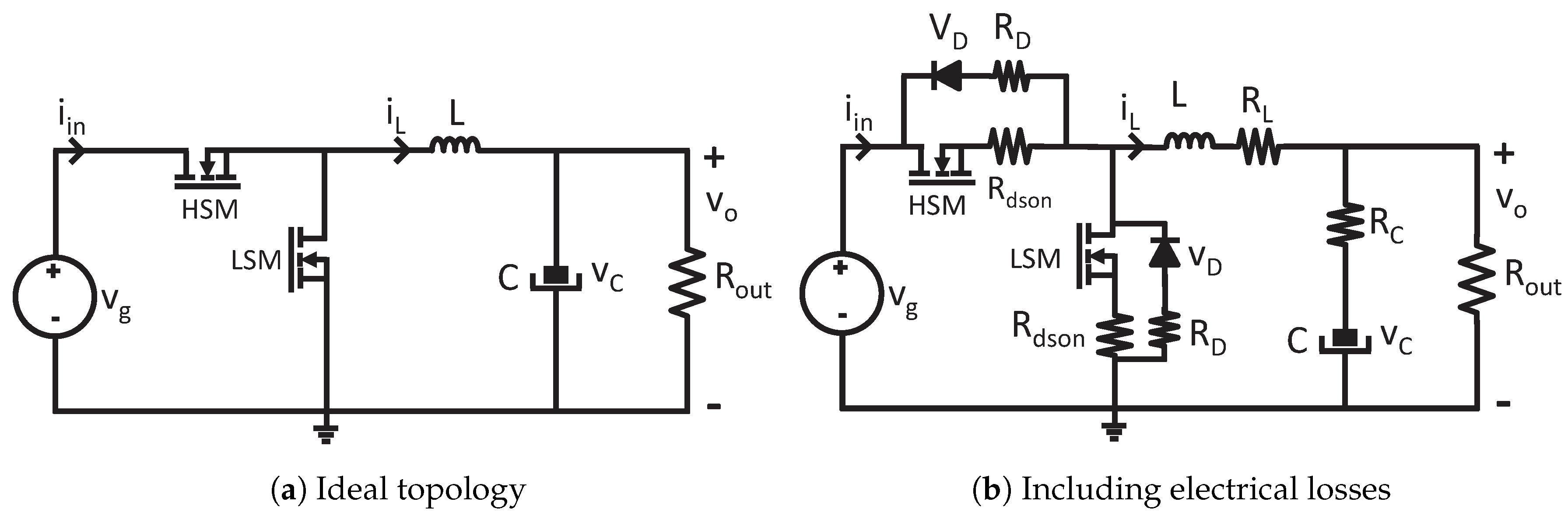
In this paper, the proposed floating-point format is applied to model a synchronous buck converter, as shown in Figure 1a. The modeling of electrical losses is not always critical for high-level simulations and many commercial tools and papers in the literature do not take them into account in order to simplify the calculi. However, there is no doubt that the inclusion of electrical losses leads to more accurate models. Therefore, in this paper, a model including electrical losses is presented, as shown in Figure 1b.

The converter can be modeled by analyzing its state variables. As there are two first-order elements—inductor and capacitor—their behaviors can be analyzed to extract the equations of the system. The voltage-current relationships of the inductors and capacitors are:

$$\{\begin{array}{l}{v}_L=L·\frac{\delta i_L}{\delta t}\\ i_C=C·\frac{\delta v_c}{\delta t}\end{array}$$

(1)

where $v_L$ and $i_L$ are the inductor voltage and current, respectively, $i_C$ and $v_C$ are the capacitor current and voltage, respectively. These ordinary differential equations (ODE) can be translated into difference equations using several numerical methods, for instance, Explicit Euler. Although there are more accurate and stable methods, Explicit Euler does not present issues when the simulation time is small enough [24]. The equations can be rearranged in order to extract the state variables, $i_L$ and $v_C$, as follows:

$$\{\begin{array}{l}{i}_L\left(k\right)=i_L(k-1)+\frac{\Delta t}{L}·v_L(k-1)\\ v_C\left(k\right)=v_C(k-1)+\frac{\Delta t}{C}·i_C(k-1)\end{array}$$

(2)

In the previous equations, $\Delta t$ is the simulation step which is constant in the proposed system. As the buck converter is a switched topology, the equations cannot be applied directly but after evaluating the states of the switches. There are two main conduction states: the conduction of high or low MOSFETs (HSM or LSM, respectively). Besides, complementary cases can be modeled when both MOSFETs are not conducting, which is usual if the controller applies deadtimes. For every case, the terms $v_L(k-1)$ and $i_C(k-1)$ are calculated before updating the state variables. In the case of the ideal model (Figure 1a), the terms $v_L(k-1)$ and $i_C(k-1)$ can be calculated as follows:

$$\{\begin{array}{l}{v}_L(k-1)=\{\begin{array}{l}{v}_g(k-1)-v_c(k-1)\Rightarrow HSM=on\&LSM=off\\ -v_c(k-1)\Rightarrow HSM=off\&LSM=on\\ v_g(k-1)-v_c(k-1)\Rightarrow HSM=off\&LSM=off\&i_L(k-1)<0\\ -v_c(k-1)\Rightarrow HSM=off\&LSM=off\&i_L(k-1)>0\\ 0\Rightarrow HSM=off\&LSM=off\&i_L(k-1)=0\end{array}\\ i_C(k-1)=i_L(k-1)-i_R(k-1)\end{array}$$

(3)

When the electrical losses are included, the equations to be applied are:

$$\{\begin{array}{l}{v}_L(k-1)=\{\begin{array}{l}{v}_g(k-1)-v_o(k-1)-i_L(k-1)\ast (R_{dson}+R_L)\Rightarrow HSM=on\&LSM=off\\ -v_o(k-1)-i_L(k-1)\ast (R_{dson}+R_L)\Rightarrow HSM=off\&LSM=on\\ v_g(k-1)-v_o(k-1)-i_L(k-1)\ast (R_d+R_L)-v_D\Rightarrow HSM=off\&\\ LSM=off\&i_L(k-1)<0\\ -v_o(k-1)-i_L(k-1)\ast (R_d+R_L)-v_D\Rightarrow HSM=off\&\\ LSM=off\&i_L(k-1)>0\\ 0\Rightarrow HSM=off\&LSM=off\&i_L(k-1)=0\end{array}\\ i_C(k-1)=i_L(k-1)-i_R(k-1)\end{array}$$

(4)

The previous equation uses the output voltage ($v_o$) instead of the capacitor voltage ($v_c$) in order to simplify the calculi. Taking into account that the output voltage should be an output of the model anyway, no more calculi are needed. $v_o$ can be calculated with the following equation:

$$v_o(k-1)=v_C(k-1)+i_C(k-1)\ast R_C$$

(5)

3. Available Standard Arithmetics for FPGAs

The equations presented in Section 2 must be applied to every simulation step. When the simulation must be executed in real-time, the latency of those operations defines the smallest simulation step that can be used. Likewise, the latency of the operations depends on the complexity of the model but also on the arithmetic that is chosen. As in software, the FPGA-based HIL implementations can use fixed-point or floating-point arithmetics. In the case of FPGAs and taking into account the VHDL language, there are three main options:

• Real type: The Real type is a non-synthesizable arithmetic which uses double-precision floating-point. As it uses 64 bits for every signal, its accuracy is good enough for any HIL simulation. However, as it cannot be synthesized into an FPGA, its use is only restricted to software simulation, not achieving real time.
• Fixed-point: Fixed-point simulations achieve optimized models in terms of latency (simulation step) and the use of hardware resources. However, the cost, in terms of design time, of implementing a model with fixed-point arithmetics is quite high, not being reasonable to use it in many cases.
• Synthesizable floating-point: This is a common choice as it is synthesizable while the design effort is reasonably low. However, the resource usage is excessively high in many cases. It can be implemented using the standard Float library included in the standard VHDL2008 [15].

As it can be deduced from the previous enumeration, standard synthesizable floating-point should be the first option in any design, and fixed-point arithmetic will be taken into account only if the user application has hard simulation step requirements. The aim of this paper is to define a new floating-point implementation optimized to be used in FPGAs, reducing the hardware resources usage. This can be achieved by removing significand roundings and normalizations, and the control of special numbers such as infinite, NaN (Not a Number), etc, which are not needed in this and many other applications.

3.1. IEEE-754 Floating-Point Basis

IEEE-754 floating-point numbers follow the format shown in Figure 2. In that standard, there is a sign bit and two other fields: exponent and significand. Merging all of them, the number is interpreted using scientific notation ($\pm significandx{2}^{exponent}$). IEEE-754 standard format is not optimized for FPGA implementation for several reasons. First of all, the number should be coded and decoded to perform a numerical operation. Besides, the number is not formatted in fixed-point (two’s complement or sign/magnitude notation), so the operations cannot take direct advantage of the embedded DSPs (Digital Signal Processor) present in FPGAs. Finally, the special number detection (NaN, infinite, etc.) adds some latency to every operation. While this detection is useful in many applications, in the case of HIL simulations of power converters, the designer does not need it.

3.2. IEEE-754 Addition, Subtraction and Multiplication

The IEEE-754 standard offers all the basic operations that can be done with real numbers: addition/subtraction, multiplication/division, arithmetic comparison, etc. The IEEE-754 standard hardware implementation is not trivial as it uses sign-magnitude notation. Besides, it is a very sequential algorithm as the exponent bias, normalization, exception handling and other features, are almost always executed in order, making it a robust but slower arithmetic. Figure 3 shows an overview of the algorithm used to perform additions, subtractions and multiplications in the IEEE-754 standard. The decomposition and composition of the number, the normalization and rounding operations and the special number detection lead to a robust but slow arithmetic for FPGA implementation.

4. LOCOFloat: Low-Cost Floating-Point Format

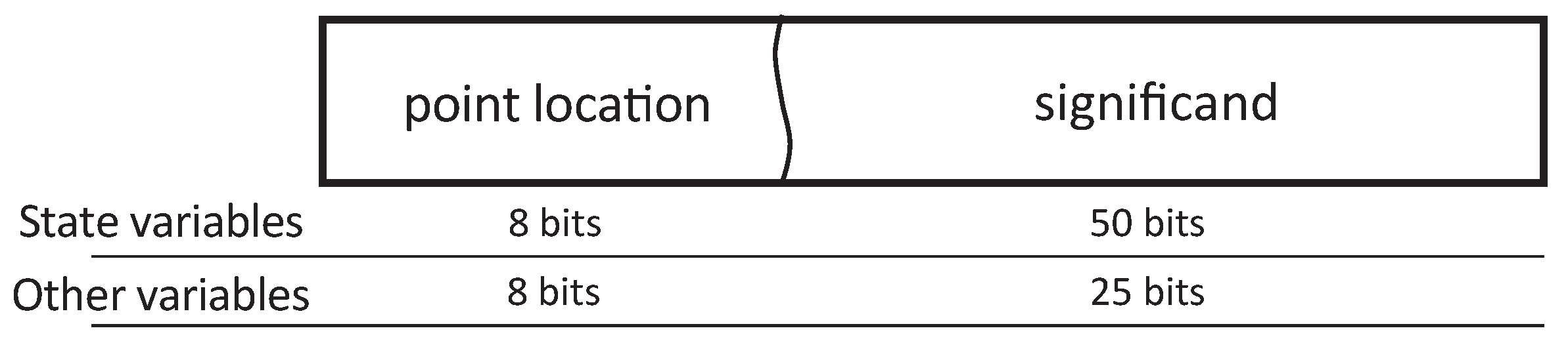
The proposed floating-point format, LOCOFloat, contains just a couple of fields: the point location—which plays the role of the exponent—and the significand, as seen in Figure 4. The former defines how many fractional bits the significand has. The latter—significand—represents the number and contains the integer and the fractional parts of the number. A higher point location field implies a smaller absolute number, contrary to the exponent field in IEEE-754. Both fields are represented in two’s complement, allowing positive and negative numbers and point locations. The width of the significand is variable, as can be seen in Figure 4, but the point location field is always represented with 8 bits in our case. Internally, the significand is virtually considered as an integer number achieving fast arithmetic operations. However, the significand indeed is a fixed-point number but with a variable point location thanks to the second field. This is why this format uses hardware resources comparable to fixed-point and well below IEEE-754 floating-point, while maintaining the advantages of floating-point.

Table 1. Examples of the proposed format.

Significand	Point Location	Binary Value	Decimal Value
${010011001001}_2$ (${1225}_{10}$)	${0000101}_2$ ($5_{10}$)	0100110.01001	38.28125
${1111111011001000}_2$ ($-{312}_{10}$)	${0000111}_2$ ($7_{10}$)	111111101.1001000	−2.4375
${011001101001}_2$ (${1641}_{10}$)	${1111010}_2$ ($-6_{10}$)	011001101001******.	105.024
${011111111001}_2$ (${2041}_{10}$)	${0101110}_2$ (${46}_{10}$)	0.00[..]011111111001	$2.900435·{10}^{-11}$

shows several examples of the proposed format. The third example of the table shows a number with a negative point location (-6) so there are six integer bits missing in the number, allowing the number to get high values. Likewise, the fourth example shows a high positive point location (46) so the number, in this case, is around ${10}^{-11}$.

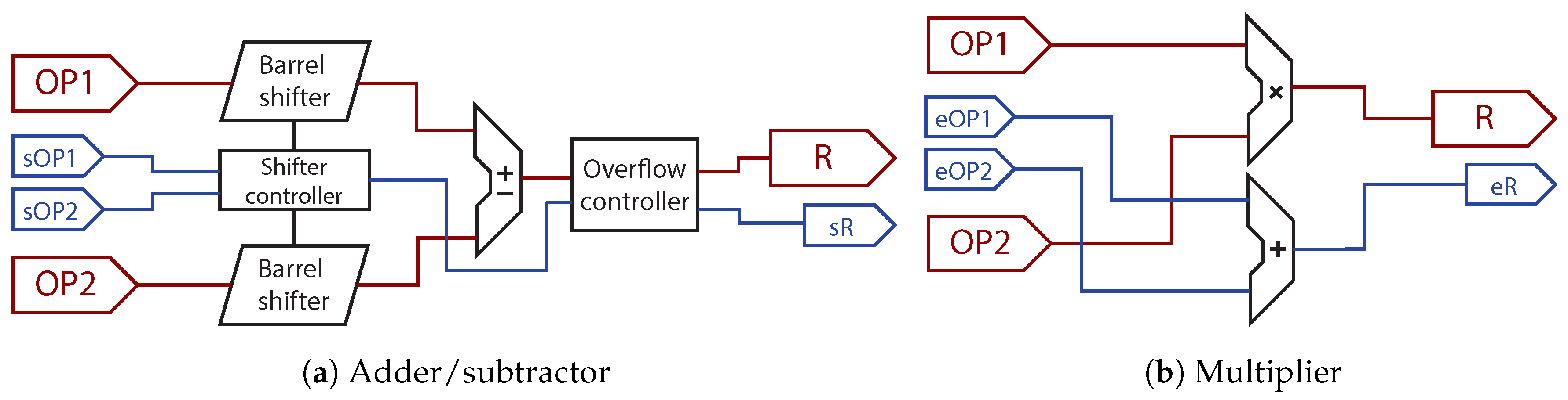
LOCOFloat is based on floating-point but its implementation is based only on two parts (significand and point location), both of them in two’s complement. Because of that, the format can be used almost directly with adders and multipliers already embedded in FPGAs. The operators defined in this paper are adapted to every possible signal width, and the width of both operands does not need to match.

Figure 5 shows the internal architecture of an adder/subtractor and a multiplier. As can be seen, all operators receive both parts of the number: significand and point location. In the case of the addition and subtraction (Figure 5a), the inputs should be point-aligned before being operated. This can be done with a barrel shifter which shifts to the right the operand with a greater number of fractional bits. The number with more fractional bits is the one that is right-shifted so a right shift aligns the point locations. A left shift of the number with fewer fractional bits cannot be done because overflow may be produced. The barrel shifters are implemented with six conditional shifters in series that provide 0–63 bit shifts controlled by six control bits called $S{h}_x$, as it can be seen in Figure 6. The barrel shifters are managed by the Shifter Controller seen in Figure 5a. For instance, if the point location of OP1 is 15 while the point location of OP2 is 3, OP1 should be right shifted 12 places. Therefore, the Shifter Controller will generate the following control command for the barrel shifter: $S{h}_{5}S{h}_{4}S{h}_{3}S{h}_{2}S{h}_{1}S{h}_0=001100$.

After aligning the points, the numbers can be added or subtracted, and the resulting point location is equal to the lowest operand point location. An overflow checking should be implemented after the operation and, if needed, the result is right-shifted one bit, adjusting the point location. Finally, as it will be seen at the end of this section, this method implements a soft-normalization, where the results are shifted one bit every clock cycle instead of implementing a variable shift.

Regarding the latency, the barrel shift to align the points before the operation is composed of $lo{g}_2\left(n\right)$ multiplexers, where n is the number of bits of the operand. Apart from the multiplexers, there are also $lo{g}_2\left(n\right)$ shifters with fixed shifting so they are quite fast. The arithmetic operation of addition/subtraction can be done in the DSPs embedded in the FPGA or it can be implemented with the logic resources of the FPGA which have also an optimized architecture for both operations. Finally, the overflow controller only adds a multiplexer and a simple -1 adder in the case that an overflow is detected—so the point should be adjusted. The latency and area results of the proposed operations are shown in Section 5.

Figure 5b shows the proposed architecture of the multiplier, which is simpler. In the case of the multiplication, the significands can be multiplied directly without any alignment. Likewise, the numbers of fractional bits are added directly, obtaining the final point location. In this case, overflow is not possible as the result size will be the sum of both input operands, so no control is needed. Therefore, there are two arithmetic modules inside a multiplication. As both are executed in parallel, their latencies are not added, but only the biggest is taken into account. The multiplication can be also implemented using the DSPs embedded in the FPGA.

As it was mentioned before, the proposed architecture allows the user to decide the width of every operand. However, those widths affect the latency of the blocks. If the designer chooses operands which fit into the FPGA DSPs, the latency can be notably lower. For instance, the latency of addition using the DSPs of a Xilinx Artix 7 FPGA (speed grade 1) is around 2 ns, while the latency of multiplication is around 5 ns [25]. Those latencies only take into account the core addition or multiplication of the module, without the rest of the logic of the proposed format, or the routing delay.

The point location checking of the addition and subtraction is conservative, just aligning the points, and the last overflow control avoids that overflow condition but it does not guarantee that the result is written in an optimal notation. In other words, one number can be written in many ways, like 4.5, which can be written with “0001001” with 1 fractional bit, with “0010010” with two fractional bits, or “0100100” with 3 fractional bits, for example. As in the next additions or subtractions, shift alignment may be done, it is better to store the number with the highest possible number of fractional bits, in a process similar to normalization. Instead of including this normalization in every operation, it is included in the state variables storage. After some calculi, the value will be written in the state variables, as it was shown in Equation (4). Just before that, this format applies a soft normalization. Trying to obtain in one step a number starting with “01” for positive or “10” for negative values would lead to many possible different shifts. In order to reduce resources and latency, LOCOFloat only shifts one position per clock cycle if the value to be stored in the register (state variable) is not normalized, following

Table 2. Soft normalization rules for LOCOFloat.

Number Leading with	Action	Explanation	Example
			Before soft-norm	After soft-norm
00	Left shift	Positive number with	Mantissa: 00001010010	Mantissa: 00010100100
		suboptimal notation	Point location: 6	Point location: 7
11	Left shift	Negative number with	Mantissa: 110100101101	Mantissa: 10100101101
		suboptimal notation	Point location: 4	Point location: 5
Other	Nothing	No overflow risk	Mantissa: 011100110101	Mantissa: 011100110101
possibilities			Point location: 7	Point location: 7

. In the second and third examples of the table, the final normalization is obtained in one single cycle. However, in the first example, several cycles will be necessary until the optimum format is reached. As the normalization is applied only to state variables, which have only smalls variations from cycle to cycle, this limitation does not affect the overall accuracy. The only case in which the soft normalization is suboptimal is when the state variable value is changed by a factor greater than 2 in a single cycle. Right shifters are not needed for soft normalization because the proposed operations already make right shifts when it is necessary. The soft normalization is enough in this application but other applications may require hard normalization. In that case, another barrel shifter would be included instead.

The proposed implementation of this numerical format is without pipelining. In all equations shown in Equation (4), the state variables need their previous value or the value from the other state variable. Therefore, the pipeline approach is not useful in this application, where the latency, but not the throughput, is important. Considering that no pipelining is used, the soft normalization in the state variables can move the point location one place in every operation—which corresponds to one clock cycle.

5. Experimental Results

In this section the implementation details of a synchronous buck converter with losses are explained. Besides, a thorough comparison between 32-bit and 64-bit standard floating-point and LOCOHIL is accomplished. The state variables should be updated every simulation step and, in the proposed model, the simulation step is directly managed by the system clock.

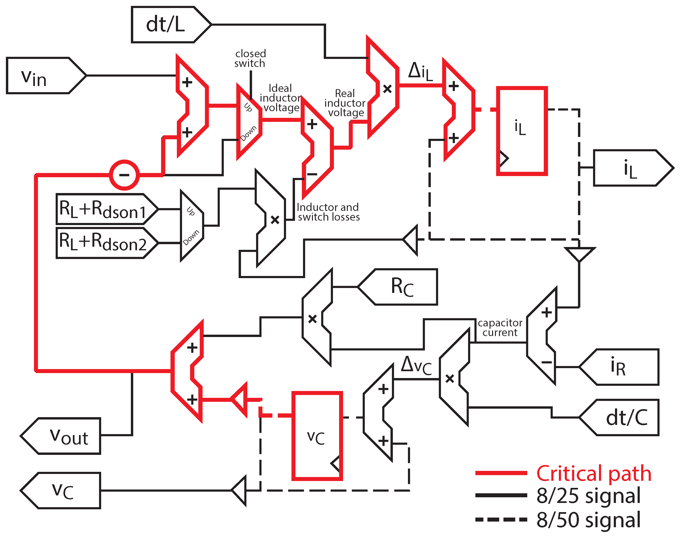
Figure 7 shows the architecture of the proposed buck converter model with losses. The implementation is a direct translation to digital electronics of the equation system (4). The choice between different formulas is done with multiplexers, and the state variables are stored in registers. All the signals but the state variables are represented in LOCOFloat with 25 bits for the significand field and 8 for the exponent (8/25 signals marked with continuous line in Figure 7). 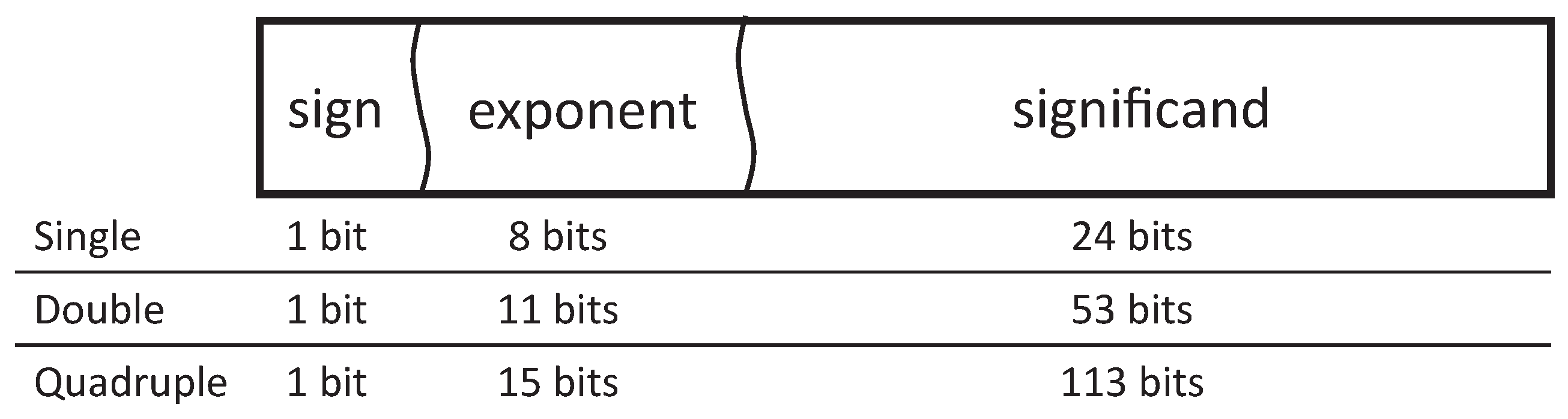The state variables, as they need much more resolution, as explained in [16], have 50 bits for the significand and 8 for the exponent (8/50 signals marked with dashed lines in Figure 7). Therefore, the accuracy obtained is equivalent to IEEE-754 with a custom format of 1 sign bit, 8 exponent bits and 48 significand bits in the state variables, and 23 significand bits for the rest of variables. The two-bit difference in the significand field between LOCOFloat and IEEE-754 comes from the sign bit—embedded in LOCOFloat—and that LOCOFLoat does not have any implicit “1” in the most significant bit of the significand.

The minimum simulation step that can be achieved depends on the complexity of the model and the arithmetic that is used. In particular, the minimum simulation step is defined by the critical path, that is, the path with the longest delay between two registers. In the proposed implementation, the critical path starts in the register that outputs the capacitor voltage value ($v_C$) and finishes in the input of the register that stores the inductor current ($i_L$). This critical path has been marked in the figure.

The 32-bit and 64-bit standard floating-point and LOCOFloat models have been implemented in a Xilinx FPGA Zynq 7 (XC7Z010-1CLG400C) in order to get the utilization of the device and the minimum simulation step. All models have been implemented using the standard VHDL-2008 and the IDE Vivado 2018.3 with the standard Xilinx synthesizer.

Table 3. FPGA (Xilinx XC7Z010-1CLG400C) resources used by the design, and percentage value with respect to the available resources in the FPGA.

System	Min Simulation Step	6-Input LUTs	FFs	DSPs
LOCOFloat	$38.973$ ns	2017	150	8
		$11.5\%$	$0.4\%$	$10\%$
32-bit Floating-point	$19.778$ ns	306	112	12
		$1.7\%$	$0.3\%$	$15\%$
64-bit Floating-point	$28.178$ ns	614	192	50
		$3.5\%$	$0.5\%$	$62.5\%$
Fixed-Point	$35.339$ ns	586	98	7
		$3.3\%$	$0.3\%$	$8.7\%$
LOCOFloat	$42.433$ ns	4693	150	0
no DSPs		$26.7\%$	$0.4\%$	$0\%$
32-bit Floating-point	$22.943$ ns	3147	115	0
no DSPs		$17.9\%$	$0.3\%$	$0\%$
64-bit Floating-point	$31.452$ ns	11277	212	0
no DSPs		$64.1\%$	$0.6\%$	$0\%$
Fixed-Point	$37.730$ ns	1536	98	0
no DSPs		%	%	$0\%$

shows the synthesis results of the model using all the considered arithmetics. Although it is not the main aim of this paper, a fixed-point implementation has been also included in Table 3 to compare it with the LOCOFloat and floating-point approaches. For the fixed-point design, the standard fixed_pkg of VHDL-2008 is used and the widths in the state variables are 50 bits while the inputs are 25-bit wide, like in LOCOFloat. It can be shown that LOCOFloat is slower than the standard floating-point arithmetic and it uses more LUTS, but the DSP usage is drastically reduced, especially when it is compared with 64-bit floating point ($84\%$ fewer DSPs). It should be noticed that DSP usage is the first limit reached by these arithmetic-based designs. Hence, the 64-bit floating-point model will be constrained by the number of DSPs available in the FPGA, not allowing the designer to implement complex power converter models. On the other hand, the hardware usage of LOCOFloat and 32-bit floating point is reasonable, so both could be used in HIL modeling for power converters. Regarding latency, it can be seen that standard floating-point is faster than LOCOFLoat, but it is mainly due to the extensive DSP usage, which noticeably accelerates the operations.

Compared with fixed-point, LOCOFloat needs considerably more LUTs, because of the barrel shifters and normalization process, and almost the same DSPs. The latency is very similar using the standard fixed_pkg or LOCOFloat. Although LOCOFloat includes soft normalization and barrel shifters, the fixed_pkg also includes rounding and some extra checking that increase the latency. Taking all into account LOCOFloat is a good choice as it uses a small number of DSPs, with the flexibility of variable point location.

Table 3 also shows the synthesis results without using DSP blocks, so the global combinational logic required by all the implementations can be compared. Disabling DSP usage is not recommended because the simulation step increases, but it helps the comparison. The difference between the minimum simulation steps still remains, but in terms of LUTs, LOCOFloat provides much better results than floating point. For instance, LOCOFloat uses 58.38% fewer LUTs than 64-bit floating-point. These synthesis results show the area optimization of the proposed numerical system.

The implementation results of the main components of LOCOFloat are shown in

Table 4. Latency and hardware utilization of the main components of LOCOFloat.

	Latency LUTS	6-Input	DSPs
	64-bit Barrel shifter	$2.178$ ns	128	0
25 × 25 Multiplier	$5.554$ ns	24	2
50 + 50 Adder/Subtractor	$13.165$ ns	460	0

. The results have been calculated for 25 × 25 bit multipliers and 50 + 50 bit adders/subtractors. As it can be seen, the multiplier is more optimized because the synthesizer uses DSPs to perform the operation. The chosen FPGA has 25 × 25 18 multipliers that almost can handle one multiplication, which in this example contains 25-bit operands. Therefore, the additional logic because of the extra length of just one operand is not so big. The addition and subtraction latencies are noticeable higher because the operand lengths are very high and because of the point alignment and overflow control, as it was shown in Figure 5. This point alignment is done with a barrel shifter, so its latency—also shown—is also included in the adder/subtractor latency.

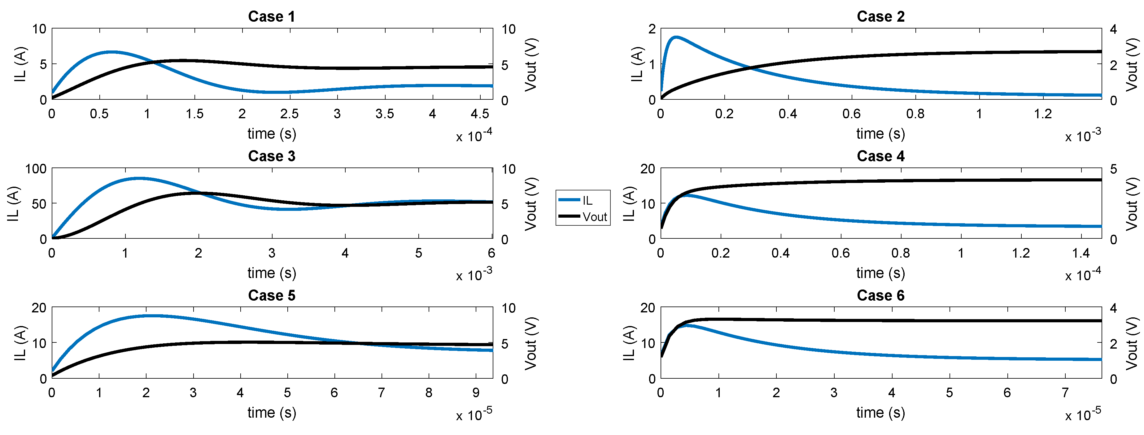
Regarding the accuracy results, this section presents a comparison between the proposed format and 32-bit and 64-bit floating-point arithmetics. In order to get a wide view of applications, six different configurations of the buck converter are considered in this section, as

Table 5. Buck parameters used in the Results section.

Case	C	L	${\mathit{V}}_{\mathit{in}}$	${\mathit{V}}_{\mathit{out}}$	P	${\mathit{F}}_{\mathit{sw}}$
1 [27]	100 $\mathsf{\mu }$F	22 $\mathsf{\mu }$H	62 V	5 V	10 W	210 kHz
2 [26]	220 $\mathsf{\mu }$F	22 $\mathsf{\mu }$H	$3.3$ V	$2.8$ V	$0.27$ W	300 kHz
3 [28]	$8.8$ mF	40 $\mathsf{\mu }$H	12 V	$5.2$ V	250 W	150 kHz
4 [29]	94 $\mathsf{\mu }$F	1 $\mathsf{\mu }$H	$5.4$ V	$4.5$ V	20 W	700 kHz
5 [30]	100 $\mathsf{\mu }$F	$2.2$$\mathsf{\mu }$H	$5.5$ V	$4.7$ V	40 W	550 kHz
5 [31]	66 $\mathsf{\mu }$F	$0.33$$\mathsf{\mu }$H	$3.9$ V	$3.25$ V	33 W	700 kHz

shows. These configurations are recommended in the application notes of the following commercial buck controllers from Maxim [26], Linear Technology [27,28] and Analog Devices [29,30,31]. It is important to mention that the models should be tested in open loop, without any controller. If a controller were present, moderate errors in the model would be compensated by the regulator, making the regulator change its actuation but getting the expected results in the state variables of the model.

Every case in Table 5 has been simulated using LOCOFLoat, the 32-bit and 64-bit floating-point (FP) arithmetics and also a reference model. The reference model implements the same equations but using the VHDL real type, which uses double-precision floating-point (variables of 64 bits), and using a much smaller simulation step (1 ns) so its accuracy is much better. All the arithmetics have been simulated using the same simulation step: 40 ns, which is the minimum simulation step that can be executed in all the arithmetics. Figure 8 shows the simulations that have been carried out related to the cases shown in Table 5. In all of them, a transient from switch-off to the nominal state has been executed. As it can be noticed, the chosen cases have very different dynamics, having a wide range of simulations to test. All the methods have been simulated and their outputs have been sampled every 10 ns and their averages in every switching cycle have been extracted. Finally, the average values have been compared to the reference model done with real type. 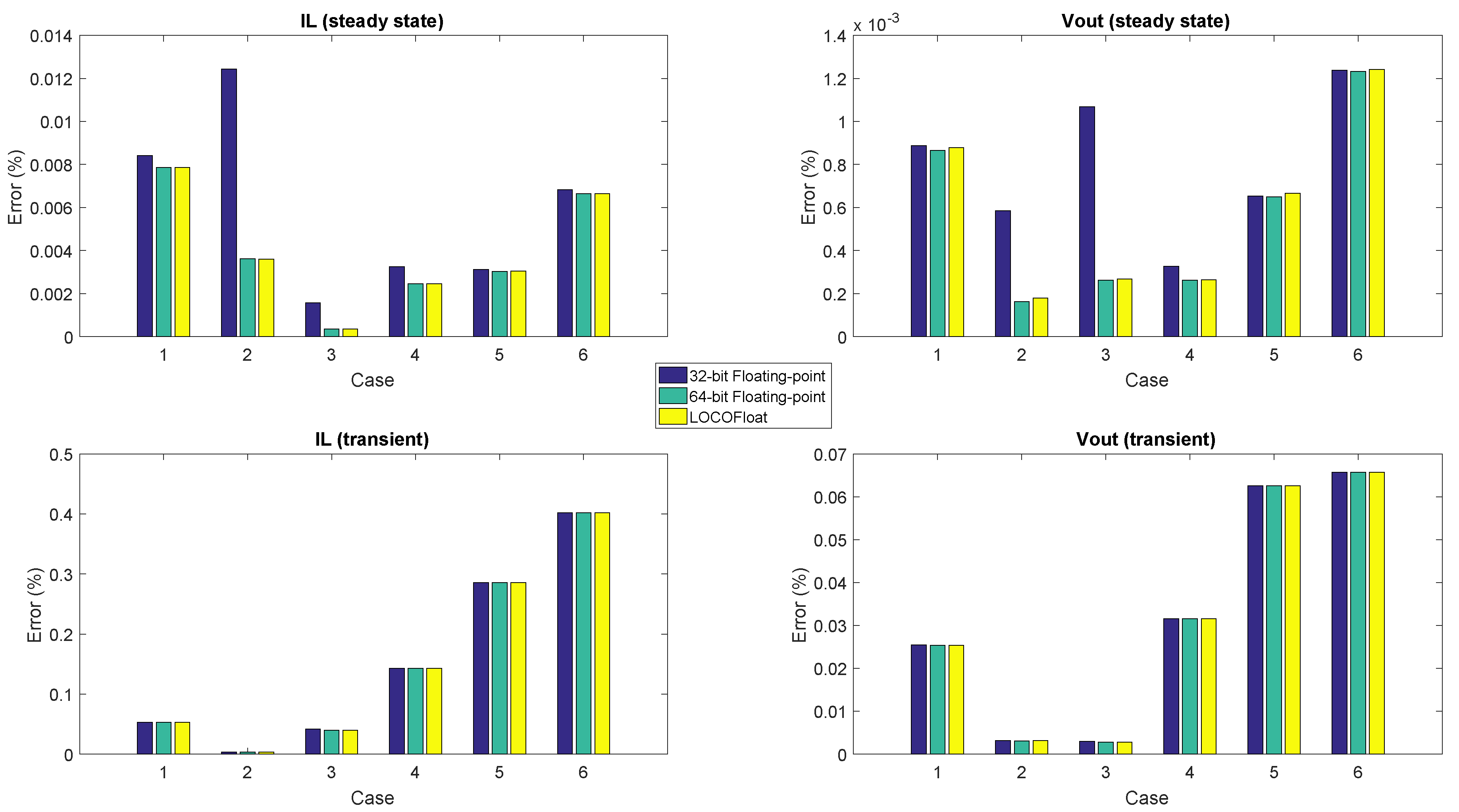Figure 9 shows the percentage error—related to the steady state values of inductor current ($i_L$) and output voltage ($v_{out}$) in the reference model—of every method for the 6 cases. The figure shows that all the arithmetics get almost the same results during the transient. However, in steady state 32-bit floating-point gets slightly more error in cases 1, 4, 5 and 6, and a big noticeable error in cases 2 and 3. This is due to resolution issues with that arithmetic. While in the transients, the incremental values are bigger, so those increments are nearer to the present current/voltage, in steady state those increments are much smaller, so a longer significand field is required to store simultaneously the present value and its increment. The numerical issues in 32-bit floating-point reach an inductor current error around $0.012\%$ in steady state in case 2. Although this error is not so high, examples of low-resolution problems with big impact using 32-bit floating point can be found in the literature, like in [16], where a boost converter using PFC (Power Factor Correction) was modeled. Therefore, 32-bit floating-point cannot be used in some applications and, as the user application is not known a priori, the most conservative choice is not to use it anyway. However, 64-bit floating-point (which has 53 bits for the significand) and LOCOFloat (which uses 50-bit state variables) can be used with guarantees.

The previous simulation was done using the same simulation step for all the arithmetics (40 ns). However, Table 3 showed that the minimum achievable simulation step for each arithmetic is different. Consequently, the arithmetics have been also simulated using the minimum simulation steps that they can get, i.e., 20 ns, 30 ns and 40 ns for 32-bit FP, 64-bit FP, and the proposed format, respectively. It should be noticed that the sources of error in the simulation may be produced by two main factors: simulation step and numerical resolution. As it was seen, the chosen arithmetic obviously determines the numerical resolution of the method. On the other hand, the error made by the ODE solver is linearly proportional to the simulation step, as Explicit Euler is used [24]. The percentage error—also related to the steady state values of $i_L$ and $v_{out}$ of the reference model—of the methods is shown in Figure 10. If there were no resolution problems, all the methods would behave as expected, where the error is proportional to the simulation step, so the best method should be the 32-bit FP, as it has the smallest simulation step. However, it can be seen that the resolution problems in 32-bit floating-point become more noticeable. The reason is that now the simulation step for that model is 20 ns, so the increments are even farther than the present state variable values. The other methods (64-bit floating-point and LOCOFloat) do not present resolution problems. To help the comparison, horizontal lines have been added taken the 64-bit FP as the reference, and showing the error that 32-bit FP and LOCOFloat are supposed to have—32-bit FP error should be around $33\%$ lower, and LOCOFloat should be around $33\%$ higher. As can be seen, the 32-bit floating-point has resolution problems not only in cases 2 and 3, so these proportions are almost never met. However, for LOCOFLoat this proportion is met, showing that the difference of error is caused only by the simulation step and not because of resolution problems.

Taking the synthesis and accuracy results, some considerations can be obtained. A 32-bit floating-point is the fastest arithmetic ($T_{clk}=20$ ns) while it does not use so many resources (12 DSPs, $15\%$ of available ones). However, its accuracy problems appear in several cases and they are difficult to predict, so this architecture is not reliable when small simulation steps are used. A 64-bit floating-point is still quite fast ($T_{clk}=30$ ns) but it uses a huge number of DSPS (50) which are the $62.5\%$ of DSPs available in the FPGA that has been used. It makes the 64-bit floating-point an unfeasible arithmetic for complex HIL models, especially in low-cost HIL systems, as the model has to fit in the FPGA. LOCOFloat is slower ($T_{clk}=40$ ns) and it uses more LUTs ($11.5\%$ of the FPGA), but the use of DSPs is very moderated (eight DSPs, $10\%$). Therefore LOCOFloat is a real alternative to be used for low-cost HIL applications.

6. Conclusions

This paper has proposed a format called LOCOFloat: Low-Cost Floating-point. The proposed format implements a floating-point library that offers the simplest operations needed in HIL: addition, subtraction and multiplication and soft normalization, with the aim of reducing the hardware requirements. It has been designed reducing the overhead of IEEE-754 floating-point standard which implements a lot of operators, with many special cases checking (e.g., NaN: Not a Number checks), rounding and hard normalization. An application example of a buck converter model with electrical losses has been used to extract the hardware usage of the proposed format, and 32-bit and 64-bit versions of IEEE-754 floating-point. Results have shown that the standard 32-bit floating-point is not reliable with small simulation steps because it suffers resolution problems. On the other hand, LOCOFloat, which uses a 50-bit mantissa field, and 64-bit floating-point are both very accurate but they offer very different hardware resources. While IEEE-754 64-bit floating-point is faster ($T_{CLK}=30$ ns instead of $T_{CLK}=40$ ns in the case of LOCOFloat), it uses many more DSPs (50 instead of eight DSPs used by LOCOFloat). Taking into account that the model of the application example is quite simple, the conclusion is that the 64-bit floating-point could not be used in many applications. Therefore, LOCOFloat is a good alternative to be used when both accuracy and low-area implementation are important.