Utilising Deep Learning Techniques for Effective Zero-Day Attack Detection

 ,
,  ,
,  ,
,  , and
, and 
Abstract
:1. Introduction
- Proposing and implementing an original and effective autoencoders model for zero-day detection IDS.
- Building an outlier detection One-Class SVM model.
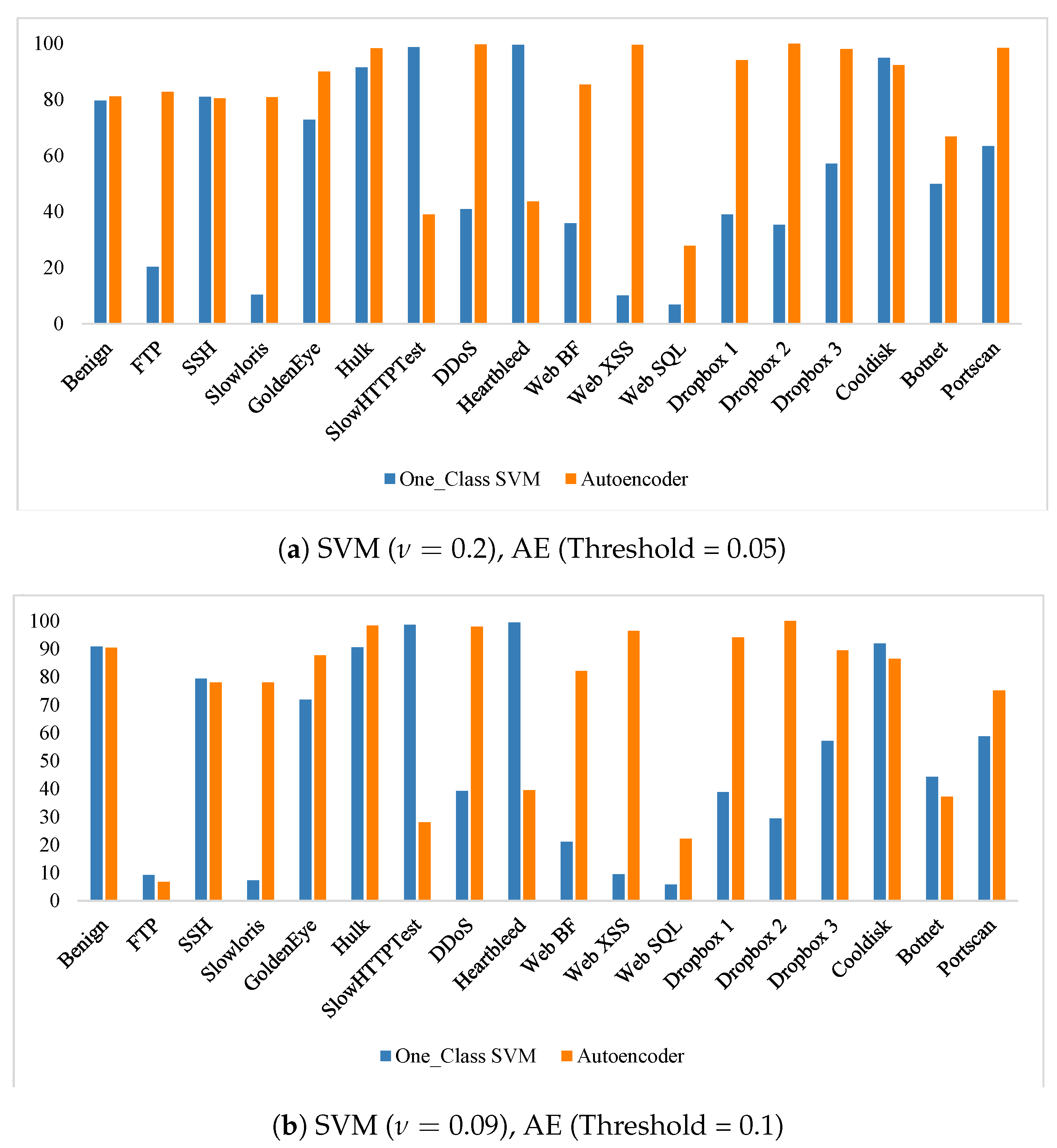
- Comparing the performance of the One-Class SVM model as a baseline outlier-based detector to the proposed Autoencoder model.
2. Background
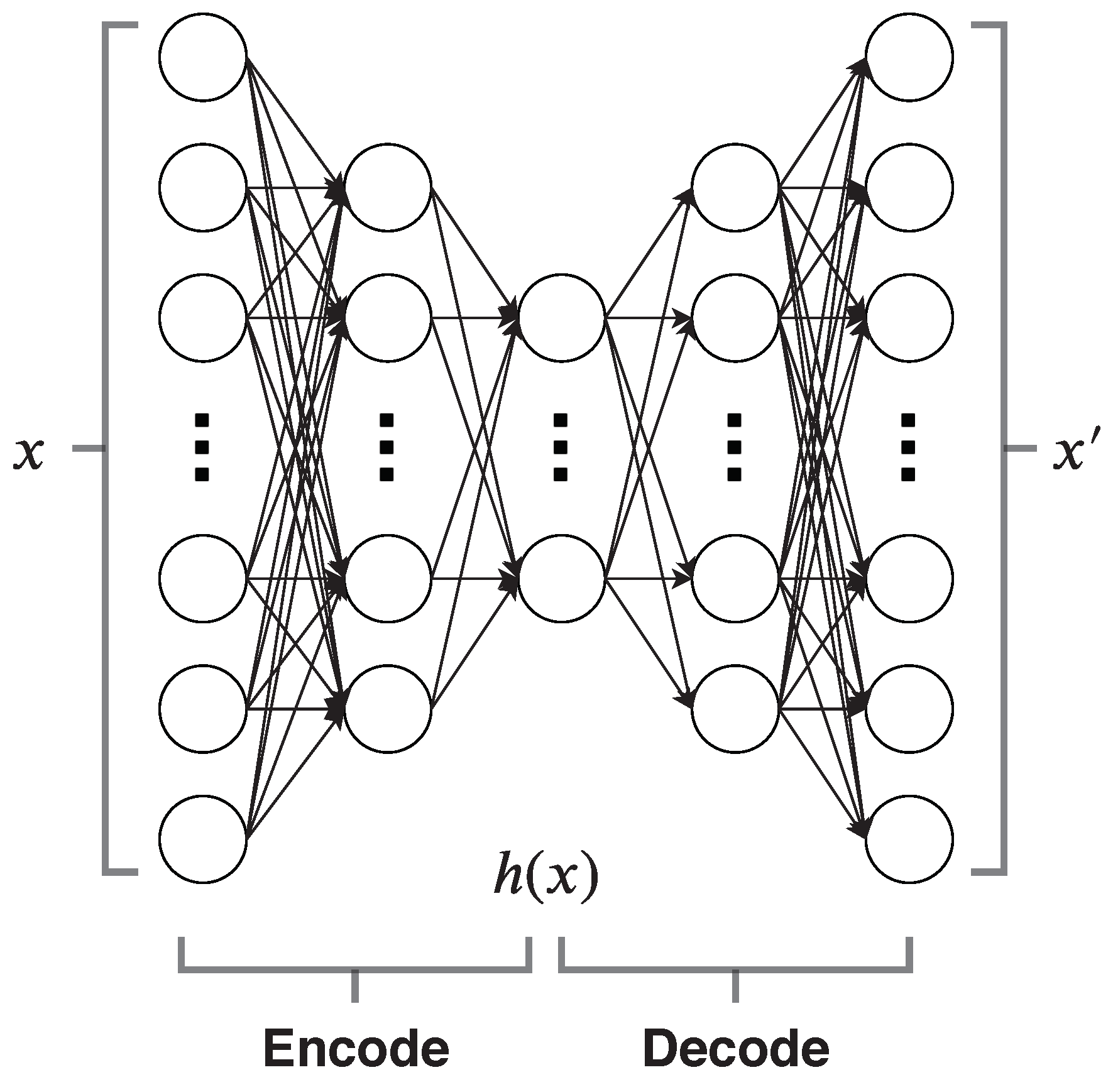
2.1. Autoencoders
2.2. One-Class SVM
3. Related Work
4. Datasets
5. Methodology, Approach and Proposed Models
5.1. CICIDS2017 Pre-Processing
| Algorithm 1 Drop correlated features |
Input: Benign Data 2D Array, N, Correlation Threshold Output: Benign Data 2D Array, Dropped Columns
|
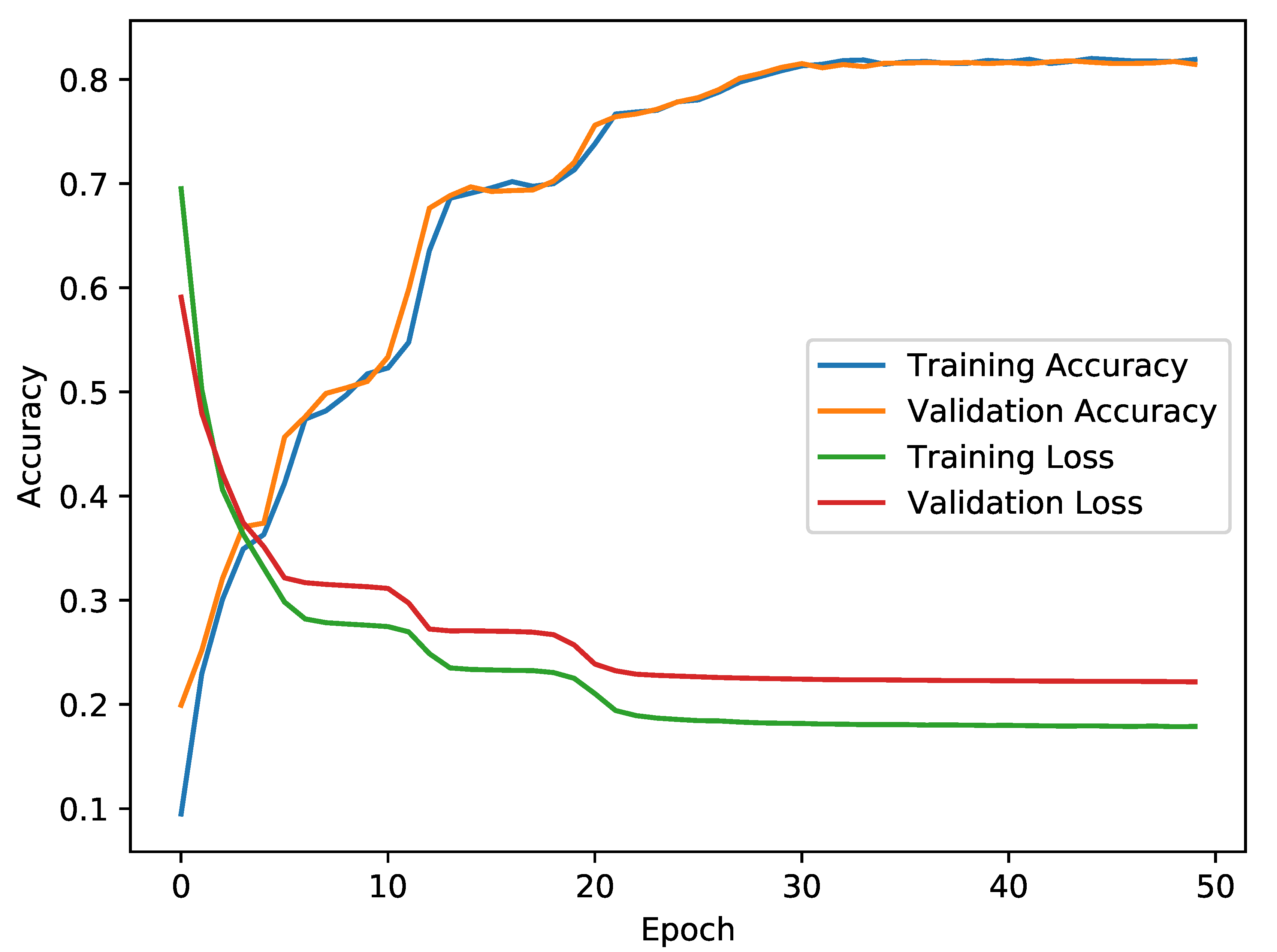
5.2. Autoencoder-Based Model
| Algorithm 2 Autoencoder Training |
Input: benign_data, ANN_architecture, regularisation_value, num_epochs Output: Trained Autoencoder
|
| Algorithm 3 Evaluation |
Input: Trained Autoencoder, attack, thresholds Output: Detection accuracies
|
5.3. One-Class SVM Based Model
| Algorithm 4 One-Class SVM Model |
Input: benign_data, nu_value Output: Trained SVM
|
6. Experimental Results
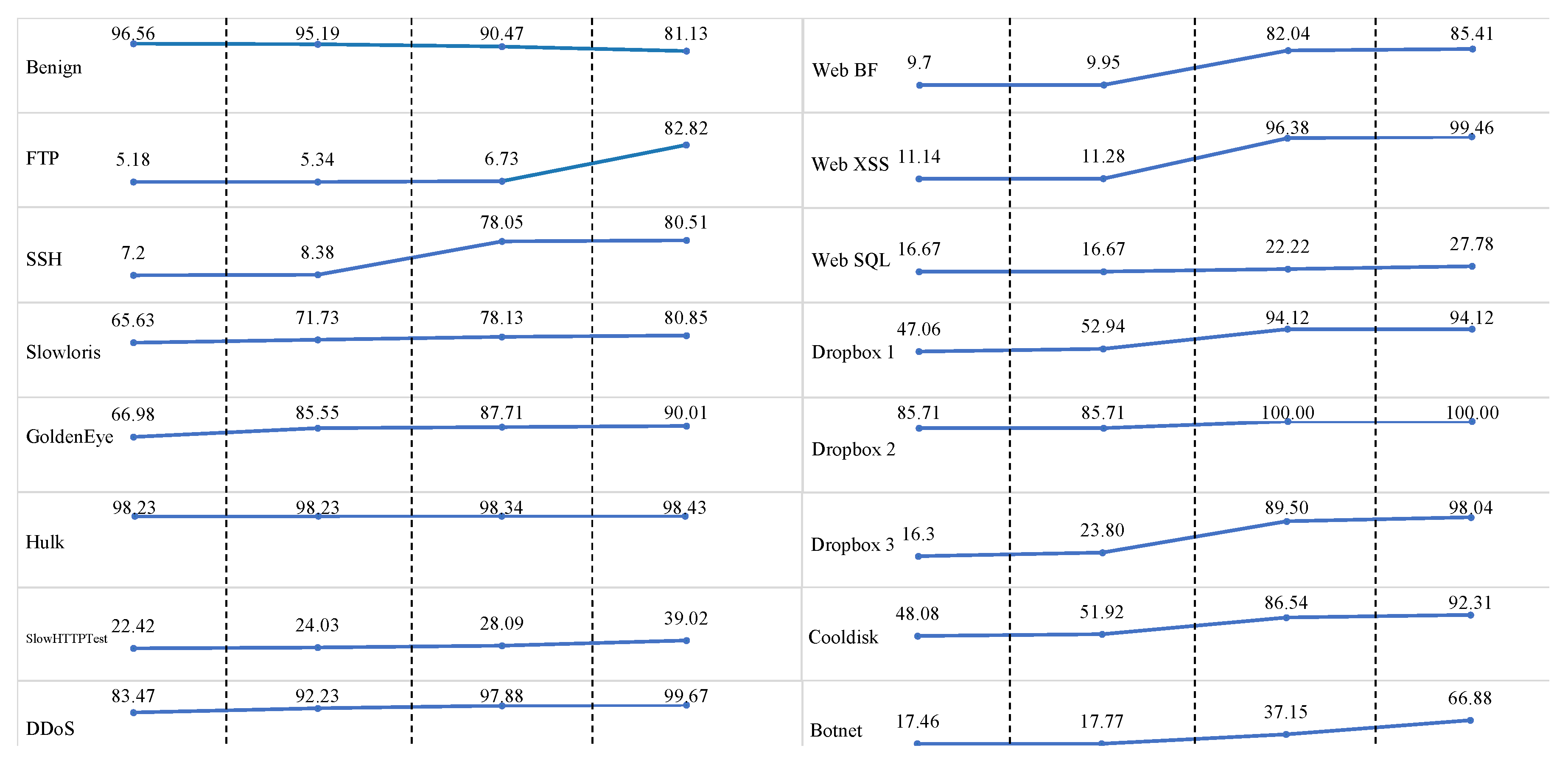
6.1. CICIDS2017 Autoencoder Results
6.2. CICIDS2017 One-Class SVM Results
6.3. NSL-KDD Results
7. Conclusions and Future Work
Author Contributions
Funding
Conflicts of Interest
References
- Kaloudi, N.; Li, J. The AI-Based Cyber Threat Landscape: A Survey. ACM Comput. Surv. 2020, 53. [Google Scholar] [CrossRef] [Green Version]
- Hindy, H.; Hodo, E.; Bayne, E.; Seeam, A.; Atkinson, R.; Bellekens, X. A Taxonomy of Malicious Traffic for Intrusion Detection Systems. In Proceedings of the 2018 International Conference On Cyber Situational Awareness, Data Analytics and Assessment (Cyber SA), Glasgow, UK, 11–12 June 2018; pp. 1–4. [Google Scholar]
- Khraisat, A.; Gondal, I.; Vamplew, P.; Kamruzzaman, J. Survey of Intrusion Detection Systems: Techniques, Datasets and Challenges. Cybersecurity 2019, 2, 20. [Google Scholar] [CrossRef]
- Hindy, H.; Brosset, D.; Bayne, E.; Seeam, A.; Tachtatzis, C.; Atkinson, R.; Bellekens, X. A Taxonomy and Survey of Intrusion Detection System Design Techniques, Network Threats and Datasets. arXiv 2018, arXiv:1806.03517. [Google Scholar]
- Chapman, C. Chapter 1—Introduction to Practical Security and Performance Testing. In Network Performance and Security; Chapman, C., Ed.; Syngress: Boston, MA, USA, 2016; pp. 1–14. [Google Scholar] [CrossRef]
- Bilge, L.; Dumitraş, T. Before We Knew It: An Empirical Study of Zero-Day Attacks in the Real World. In Proceedings of the 2012 ACM Conference on Computer and Communications Security (CCS ’12), Raleigh, NC, USA, 16–18 October 2012; pp. 833–844. [Google Scholar] [CrossRef]
- Nguyen, T.T.; Reddi, V.J. Deep Reinforcement Learning for Cyber Security. arXiv 2019, arXiv:1906.05799. [Google Scholar]
- Metrick, K.; Najafi, P.; Semrau, J. Zero-Day Exploitation Increasingly Demonstrates Access to Money, Rather than Skill—Intelligence for Vulnerability Management; Part One; FireEye Inc.: Milpitas, CA, USA, 2020. [Google Scholar]
- Cisco. Cisco 2017 Annual Cyber Security Report. 2017. Available online: https://www.grouppbs.com/wp-content/uploads/2017/02/Cisco_2017_ACR_PDF.pdf (accessed on 20 July 2020).
- Ficke, E.; Schweitzer, K.M.; Bateman, R.M.; Xu, S. Analyzing Root Causes of Intrusion Detection False-Negatives: Methodology and Case Study. In Proceedings of the 2019 IEEE Military Communications Conference (MILCOM), Norfolk, VA, USA, 12–14 November 2019; pp. 1–6. [Google Scholar]
- Sharma, V.; Kim, J.; Kwon, S.; You, I.; Lee, K.; Yim, K. A Framework for Mitigating Zero-Day Attacks in IoT. arXiv 2018, arXiv:1804.05549. [Google Scholar]
- Sun, X.; Dai, J.; Liu, P.; Singhal, A.; Yen, J. Using Bayesian Networks for Probabilistic Identification of Zero-Day Attack Paths. IEEE Trans. Inf. Forensics Secur. 2018, 13, 2506–2521. [Google Scholar] [CrossRef]
- Zhou, Q.; Pezaros, D. Evaluation of Machine Learning Classifiers for Zero-Day Intrusion Detection–An Analysis on CIC-AWS-2018 dataset. arXiv 2019, arXiv:1905.03685. [Google Scholar]
- Zhao, J.; Shetty, S.; Pan, J.W.; Kamhoua, C.; Kwiat, K. Transfer Learning for Detecting Unknown Network Attacks. EURASIP J. Inf. Secur. 2019, 2019, 1. [Google Scholar] [CrossRef]
- Sameera, N.; Shashi, M. Deep Transductive Transfer Learning Framework for Zero-Day Attack Detection. ICT Express 2020. [Google Scholar] [CrossRef]
- Abri, F.; Siami-Namini, S.; Khanghah, M.A.; Soltani, F.M.; Namin, A.S. The Performance of Machine and Deep Learning Classifiers in Detecting Zero-Day Vulnerabilities. arXiv 2019, arXiv:1911.09586. [Google Scholar]
- Kim, J.Y.; Bu, S.J.; Cho, S.B. Zero-day Malware Detection using Transferred Generative Adversarial Networks based on Deep Autoencoders. Inf. Sci. 2018, 460–461, 83–102. [Google Scholar] [CrossRef]
- Rumelhart, D.E.; Hinton, G.E.; Williams, R.J. Learning Internal Representations by Error Propagation; Technical Report; California Univ San Diego La Jolla Inst for Cognitive Science: San Diego, CA, USA, 1985. [Google Scholar]
- Stewart, M. Comprehensive Introduction to Autoencoders. 2019. Available online: https://towardsdatascience.com/generating-images-with-autoencoders-77fd3a8dd368 (accessed on 21 July 2020).
- Goodfellow, I.; Bengio, Y.; Courville, A. Deep Learning; MIT Press: Cambridge, MA, USA, 2016. [Google Scholar]
- Barber, D. Implicit Representation Networks; Technical Report; Department of Computer Science, University College London: London, UK, 2014. [Google Scholar]
- Hinton, G.E.; Salakhutdinov, R.R. Reducing the Dimensionality of Data with Neural Networks. Science 2006, 313, 504–507. [Google Scholar] [CrossRef] [PubMed] [Green Version]
- Zabalza, J.; Ren, J.; Zheng, J.; Zhao, H.; Qing, C.; Yang, Z.; Du, P.; Marshall, S. Novel Segmented Stacked Autoencoder for Effective Dimensionality Reduction and Feature Extraction in Hyperspectral Imaging. Neurocomputing 2016, 185, 1–10. [Google Scholar] [CrossRef] [Green Version]
- Liou, C.Y.; Cheng, W.C.; Liou, J.W.; Liou, D.R. Autoencoder for Words. Neurocomputing 2014, 139, 84–96. [Google Scholar] [CrossRef]
- Theis, L.; Shi, W.; Cunningham, A.; Huszár, F. Lossy Image Compression with Compressive Autoencoders. arXiv 2017, arXiv:1703.00395. [Google Scholar]
- Zhou, C.; Paffenroth, R.C. Anomaly Detection with Robust Deep Autoencoders. In Proceedings of the 23rd ACM SIGKDD International Conference on Knowledge Discovery and Data Mining, Halifax, NS, Canada, 13–17 August 2017; pp. 665–674. [Google Scholar]
- Creswell, A.; Bharath, A.A. Denoising Adversarial Autoencoders. IEEE Trans. Neural Netw. Learn. Syst. 2018, 30, 968–984. [Google Scholar] [CrossRef] [PubMed] [Green Version]
- Cortes, C.; Vapnik, V. Support-Vector Networks. Mach. Learn. 1995, 20, 273–297. [Google Scholar] [CrossRef]
- Ng, A. Part V: Support Vector Machines|CS229 Lecture Notes. 2000. Available online: http://cs229.stanford.edu/notes/cs229-notes3.pdf (accessed on 21 July 2020).
- Zisserman, A. The SVM classifier|C19 Machine Learning. 2015. Available online: https://www.robots.ox.ac.uk/~az/lectures/ml/lect2.pdf (accessed on 21 July 2020).
- Schölkopf, B.; Williamson, R.C.; Smola, A.J.; Shawe-Taylor, J.; Platt, J.C. Support Vector Method for Novelty Detection. Adv. Neural Inf. Process. Syst. 2000, 12, 582–588. [Google Scholar]
- Tax, D.M.; Duin, R.P. Support Vector Data Description. Mach. Learn. 2004, 54, 45–66. [Google Scholar] [CrossRef] [Green Version]
- Wang, S.; Liu, Q.; Zhu, E.; Porikli, F.; Yin, J. Hyperparameter Selection of One-Class Support Vector Machine by Self-Adaptive Data Shifting. Pattern Recognit. 2018, 74, 198–211. [Google Scholar] [CrossRef] [Green Version]
- Hodo, E.; Bellekens, X.; Hamilton, A.; Tachtatzis, C.; Atkinson, R. Shallow and Deep Networks Intrusion Detection System: A Taxonomy and Survey. arXiv 2017, arXiv:1701.02145. [Google Scholar]
- Hamed, T.; Ernst, J.B.; Kremer, S.C. A Survey and Taxonomy of Classifiers of Intrusion Detection Systems. In Computer and Network Security Essentials; Daimi, K., Ed.; Springer International Publishing: Cham, Switzerland, 2018; pp. 21–39. [Google Scholar] [CrossRef]
- Hindy, H.; Brosset, D.; Bayne, E.; Seeam, A.K.; Tachtatzis, C.; Atkinson, R.; Bellekens, X. A Taxonomy of Network Threats and the Effect of Current Datasets on Intrusion Detection Systems. IEEE Access 2020, 8, 104650–104675. [Google Scholar] [CrossRef]
- Buczak, A.L.; Guven, E. A Survey of Data Mining and Machine Learning Methods for Cyber Security Intrusion Detection. IEEE Commun. Surv. Tutor. 2016, 18, 1153–1176. [Google Scholar] [CrossRef]
- Aceto, G.; Ciuonzo, D.; Montieri, A.; Pescapé, A. Toward effective mobile encrypted traffic classification through deep learning. Neurocomputing 2020, 409, 306–315. [Google Scholar] [CrossRef]
- Rashid, F.Y. Encryption, Privacy in the Internet Trends Report|Decipher. 2019. Available online: https://duo.com/decipher/encryption-privacy-in-the-internet-trends-report (accessed on 14 September 2020).
- Kunang, Y.N.; Nurmaini, S.; Stiawan, D.; Zarkasi, A.; Jasmir, F. Automatic Features Extraction Using Autoencoder in Intrusion Detection System. In Proceedings of the 2018 International Conference on Electrical Engineering and Computer Science (ICECOS), Pangkal Pinang, Indonesia, 2–4 October 2018; pp. 219–224. [Google Scholar]
- Kherlenchimeg, Z.; Nakaya, N. Network Intrusion Classifier Using Autoencoder with Recurrent Neural Network. In Proceedings of the Fourth International Conference on Electronics and Software Science (ICESS2018), Takamatsu, Japan, 5–7 November 2018; pp. 94–100. [Google Scholar]
- Shaikh, R.A.; Shashikala, S. An Autoencoder and LSTM based Intrusion Detection Approach Against Denial of Service Attacks. In Proceedings of the 2019 1st International Conference on Advances in Information Technology (ICAIT), Chickmagalur, India, 25–27 July 2019; pp. 406–410. [Google Scholar]
- Abolhasanzadeh, B. Nonlinear Dimensionality Reduction for Intrusion Detection using Auto-Encoder Bottleneck Features. In Proceedings of the 2015 7th Conference on Information and Knowledge Technology (IKT), Urmia, Iran, 26–28 May 2015; pp. 1–5. [Google Scholar]
- Javaid, A.; Niyaz, Q.; Sun, W.; Alam, M. A Deep Learning Approach for Network Intrusion Detection System. In Proceedings of the 9th EAI International Conference on Bio-Inspired Information and Communications Technologies (Formerly BIONETICS), New York, NY, USA, 3–5 December 2016; pp. 21–26. [Google Scholar]
- AL-Hawawreh, M.; Moustafa, N.; Sitnikova, E. Identification of Malicious Activities In Industrial Internet of Things Based On Deep Learning Models. J. Inf. Secur. Appl. 2018, 41, 1–11. [Google Scholar] [CrossRef]
- Shone, N.; Ngoc, T.N.; Phai, V.D.; Shi, Q. A Deep Learning Approach To Network Intrusion Detection. IEEE Trans. Emerg. Top. Comput. Intell. 2018, 2, 41–50. [Google Scholar] [CrossRef] [Green Version]
- Farahnakian, F.; Heikkonen, J. A Deep Auto-encoder Based Approach for Intrusion Detection System. In Proceedings of the 2018 20th International Conference on Advanced Communication Technology (ICACT), Chuncheon, Korea, 11–14 February 2018; p. 1. [Google Scholar]
- Meidan, Y.; Bohadana, M.; Mathov, Y.; Mirsky, Y.; Shabtai, A.; Breitenbacher, D.; Elovici, Y. N-BaIoT—Network-Based Detection of IoT Botnet Attacks Using Deep Autoencoders. IEEE Pervasive Comput. 2018, 17, 12–22. [Google Scholar] [CrossRef] [Green Version]
- Bovenzi, G.; Aceto, G.; Ciuonzo, D.; Persico, V.; Pescapé, A. A Hierarchical Hybrid Intrusion Detection Approach in IoT Scenarios. Available online: https://www.researchgate.net/profile/Domenico_Ciuonzo/publication/344076571_A_Hierarchical_Hybrid_Intrusion_Detection_Approach_in_IoT_Scenarios/links/5f512e5092851c250b8e934c/A-Hierarchical-Hybrid-Intrusion-Detection-Approach-in-IoT-Scenarios.pdf (accessed on 14 September 2020).
- Canadian Institute for Cybersecurity. Intrusion Detection Evaluation Dataset (CICIDS2017). 2017. Available online: http://www.unb.ca/cic/datasets/ids-2017.html (accessed on 15 June 2018).
- Panigrahi, R.; Borah, S. A Detailed Analysis of CICIDS2017 Dataset for Designing Intrusion Detection Systems. Int. J. Eng. Technol. 2018, 7, 479–482. [Google Scholar]
- Sharafaldin, I.; Habibi Lashkari, A.; Ghorbani, A.A. A Detailed Analysis of the CICIDS2017 Data Set. In Information Systems Security and Privacy; Mori, P., Furnell, S., Camp, O., Eds.; Springer International Publishing: Cham, Switzerland, 2019; pp. 172–188. [Google Scholar]
- Canadian Institute for Cybersecurity. NSL-KDD Dataset. Available online: http://www.unb.ca/cic/datasets/nsl.html (accessed on 15 June 2018).
- Tavallaee, M.; Bagheri, E.; Lu, W.; Ghorbani, A.A. A Detailed Analysis of the KDD CUP 99 Data Set. In Proceedings of the 2009 IEEE Symposium on Computational Intelligence for Security and Defense Applications, Ottawa, ON, Canada, 8–10 July 2009; pp. 1–6. [Google Scholar]
- Tobi, A.M.A.; Duncan, I. KDD 1999 Generation Faults: A Review And Analysis. J. Cyber Secur. Technol. 2018, 1–37. [Google Scholar] [CrossRef]
- Siddique, K.; Akhtar, Z.; Khan, F.A.; Kim, Y. Kdd Cup 99 Data Sets: A Perspective on the Role of Data Sets in Network Intrusion Detection Research. Computer 2019, 52, 41–51. [Google Scholar]
- Bala, R.; Nagpal, R. A Review on KDD CUP99 and NSL-KDD Dataset. Int. J. Adv. Res. Comput. Sci. 2019, 10, 64. [Google Scholar] [CrossRef] [Green Version]
- Rezaei, S.; Liu, X. Deep Learning for Encrypted Traffic Classification: An Overview. IEEE Commun. Mag. 2019, 57, 76–81. [Google Scholar] [CrossRef] [Green Version]
- Guggisberg, S. How to Split a Dataframe into Train and Test Set with Python. 2020. Available online: https://towardsdatascience.com/how-to-split-a-dataframe-into-train-and-test-set-with-python-eaa1630ca7b3 (accessed on 17 August 2020).
- Bergstra, J.; Bengio, Y. Random Search for Hyper-parameter Optimization. J. Mach. Learn. Res. 2012, 13, 281–305. [Google Scholar]
- Liashchynskyi, P.; Liashchynskyi, P. Grid Search, Random Search, Genetic Algorithm: A Big Comparison for NAS. arXiv 2019, arXiv:1912.06059. [Google Scholar]
- Chen, P.H.; Lin, C.J.; Schölkopf, B. A Tutorial on ν-Support Vector Machines. Appl. Stoch. Model. Bus. Ind. 2005, 21, 111–136. [Google Scholar] [CrossRef]
- Gharib, M.; Mohammadi, B.; Dastgerdi, S.H.; Sabokrou, M. AutoIDS: Auto-encoder Based Method for Intrusion Detection System. arXiv 2019, arXiv:1911.03306. [Google Scholar]
- Aygun, R.C.; Yavuz, A.G. Network Anomaly Detection with Stochastically Improved Autoencoder Based Models. In Proceedings of the 2017 IEEE 4th International Conference on Cyber Security and Cloud Computing (CSCloud), New York, NY, USA, 26–28 June 2017; pp. 193–198. [Google Scholar]
Publisher’s Note: MDPI stays neutral with regard to jurisdictional claims in published maps and institutional affiliations. |


| Day | Traffic |
|---|---|
| Monday | Benign |
| Tuesday | SSH & FTP Brute Force |
| Wednesday | DoS/DDoS & Heartbleed |
| Thursday | Web Attack (Brute Force, XSS, Sql Injection) & Infiltration |
| Friday | Botnet, Portscan & DDoS |
| Class | Accuracy | ||
|---|---|---|---|
| 0.2 | 0.15 | 0.1 | |
| Benign (Validation) | 89.81% | 84.84% | 79.71% |
| FTP Bruteforce | 10.19% | 15.16% | 20.29% |
| SSH Bruteforce | 79.51% | 80.26% | 80.95% |
| DoS (Slowloris) | 7.66% | 8.38% | 10.37% |
| DoS (GoldenEye) | 71.87% | 72.39% | 72.85% |
| DoS (Hulk) | 90.69% | 91.35% | 91.55% |
| DoS (Slowhttps) | 98.59% | 98.66% | 98.71% |
| DDoS | 39.35% | 39.94% | 40.96% |
| Heartbleed | 99.49% | 99.54% | 99.58% |
| Web BF | 21.1% | 23.41% | 35.84% |
| Web XSS | 9.58% | 9.76% | 10.13% |
| Web SQL | 5.77% | 6.31% | 6.85% |
| Infiltration-Dropbox 1 | 38.89% | 38.89% | 38.89% |
| Infiltration-Dropbox 2 | 29.41% | 35.29% | 35.29% |
| Infiltration-Dropbox 3 | 57.14% | 57.14% | 57.14% |
| Infiltration-Cooldisk | 92.15% | 93.8% | 94.91% |
| Botnet | 44.23% | 46.15% | 50% |
| PortScan | 59.27% | 60.04% | 63.43% |
| Class | Accuracy | ||
|---|---|---|---|
| 0.3 | 0.25 | 0.2 | |
| KDDTrain+.csv | |||
| Normal (Validation) | 78.81% | 77.63% | 78.81% |
| DoS | 98.15% | 98.16% | 98.15% |
| Probe | 99.89% | 99.94% | 99.89% |
| R2L | 83.12% | 96.48% | 83.12% |
| U2R | 84.62% | 100% | 84.62% |
| KDDTest+.csv | |||
| Normal | 84.82% | 84.42% | 84.82% |
| DoS | 94.67% | 94.67% | 94.67% |
| Probe | 100% | 100% | 100% |
| R2L | 95.95% | 96.5% | 95.95% |
| U2R | 83.78% | 89.19% | 83.78% |
| Year | Reference | Approach | Train:Test % of KDDTrain+ | KDDTrain+ Accuracy | KDDTest+ Accuracy |
|---|---|---|---|---|---|
| This paper | AE th = 0.3 AE th = 0.25 AE th = 0.2 | 75 : 25 | 88.92% 94.44% 88.92% | 91.84% 92.96% 91.84% | |
| 2019 | [63] | 2 AEs | - | - | 90.17% |
| 2017 | [64] | AE Denoising AE | 80 : 20 | 93.62% 94.35% | 88.28% 88.65% |
| Class | Accuracy | ||
|---|---|---|---|
| 0.2 | 0.15 | 0.1 | |
| KDDTrain+.csv | |||
| Normal (Validation) | 89.9% | 85.14% | 80.54% |
| DoS | 98.13% | 98.14% | 98.14% |
| Probe | 97.74% | 98.77% | 99.52% |
| R2L | 49.35% | 52.26% | 81.71% |
| U2R | 78.85% | 80.77% | 82.69% |
| KDDTest+.csv | |||
| Normal | 88.12% | 86.02% | 84.72% |
| DoS | 94.67% | 94.67% | 94.69% |
| Probe | 99.55% | 99.91% | 100% |
| R2L | 80.17% | 82.22% | 90.31% |
| U2R | 78.38% | 78.38% | 83.78% |
© 2020 by the authors. Licensee MDPI, Basel, Switzerland. This article is an open access article distributed under the terms and conditions of the Creative Commons Attribution (CC BY) license (http://creativecommons.org/licenses/by/4.0/).
Share and Cite
Hindy, H.; Atkinson, R.; Tachtatzis, C.; Colin, J.-N.; Bayne, E.; Bellekens, X. Utilising Deep Learning Techniques for Effective Zero-Day Attack Detection. Electronics 2020, 9, 1684. https://doi.org/10.3390/electronics9101684
Hindy H, Atkinson R, Tachtatzis C, Colin J-N, Bayne E, Bellekens X. Utilising Deep Learning Techniques for Effective Zero-Day Attack Detection. Electronics. 2020; 9(10):1684. https://doi.org/10.3390/electronics9101684
Chicago/Turabian StyleHindy, Hanan, Robert Atkinson, Christos Tachtatzis, Jean-Noël Colin, Ethan Bayne, and Xavier Bellekens. 2020. "Utilising Deep Learning Techniques for Effective Zero-Day Attack Detection" Electronics 9, no. 10: 1684. https://doi.org/10.3390/electronics9101684