Abstract
The synthesis of electric motor control systems, seeking optimal performance, is a well-known and studied field of automation to date. However, the solutions often use very elaborate mathematical foundations and sometimes require considerable algorithmic complexity. Another approach to the same problem, which offers very interesting results, is the use of artificial intelligence methods to generate controllers. Intelligent methods allow the use of bio-inspired approaches to solve complex problems. This article presents a method to adjust the parameters of a controller for DC motors based on two components in the objective function: High productivity and efficiency. This can be achieved using well-known and low algorithmic complexity PID controllers, and metaheuristic artificial intelligence techniques to adjust a controller to obtain optimal behavior. To validate the benefits of the methodological proposal, a simulator of a DC motor has been rigorously constructed, respecting fundamental physical principles. The adjustment system based on metaheuristics (genetics algorithms) has been designed to work on the simulator and constitutes the central contribution of the paper. This system has been designed to establish the parameters of a PID controller, optimizing its behavior in relation to two variables of interest, such as performance and energy efficiency (a non-trivial problem). The results obtained confirm the benefits of the approach.
1. Introduction
Optimal control strategies are a branch of control theory seeking to find a controller for a dynamic system that works for a certain period of time, in such a way that an objective function that maximizes payoff is optimized and provides the best control for our system.
The basis of optimal control is the Pontryagin Maximum Principle for linear time-optimal control and its variants, which is defined as a necessary condition that a controller must meet to be optimal [1]. This principle allows us to find the optimal parameters of a system, provided that the criterion used to calculate performance is a scalar function of the parameters and state variables [2]. However, the optimization of the controller parameters can also be carried out using a non-scalar-valued performance criterion based on consideration of several cost functions simultaneously (speed, energy consumption, emissions, integral squared error, etc.).
As a result of these first advances in the field of optimal control theory, various techniques have been developed in the field of control engineering, which introduce these theoretical concepts in the development of operational control systems.
Dynamic programming is a technique to designing optimal controls, assuming that the control strategy can be designed using the Hamilton-Jacobi-Bellman nonlinear partial differential equation [3]. Additionally, numerical methods for discrete-time optimal control should be applied to obtain the adjusted parameters of the regulator [4]. If system dynamics are described by a set of linear differential equations and the cost function to support the optimization is described by a quadratic function, the problem is called linear-quadratic (LQ), and its associated optimum controller is called a linear-quadratic regulator (LQR) [5].
These control methods require a very specific preparation, as they are supported by advanced-level knowledge, which complicates their general use. Moreover, the solutions proposed may also be complicated from an algorithmic point of view, since the controller may be forced to recalculate parameters in each execution cycle (i.e., optimal finite horizon control).
Consequently, in recent years, alternative techniques based on artificial intelligence (AI) have been applied to obtain a solution to the problem of optimal control. Therefore, in [6], a system for the optimization of the parameters of a simple proportional-integral-derivative (PID) controller is presented by using a genetic algorithm, particle swarm optimization, and the method of cross entropy with very simple models and basic error measurements, based on the root mean square. A similar but a slightly more complex approach is followed in [7], where a series of metaheuristics (genetic algorithms and particle swarm optimizers) are used to optimize the gains of a Gaussian adaptive PID controller. A much more extensive analysis of these methods is carried out in a survey of the applicability of these techniques [8], which indicates the greatest challenges in the field in systems with multi-objective optimization.
However, both the numerical, analytical, and AI-based approaches have one factor in common: The definition of the corresponding cost function as the basis for optimizing control systems in the event that multiple parameters are to be optimized simultaneously [9]. There is no clear methodology for the definition and modeling of this cost function, nor for its adaptation to each of the techniques to be used.
Metaheuristics is an AI-based technique that refers to optimal search procedures within a multidimensional space, which include various sets of techniques, including some that are bio-inspired. A common characteristic that they share is that they do not require the function to be optimized to be differentiable [10]. A typical field of application of metaheuristics is combinatorial optimization, although it can also be applied to numerical optimization problems, as is the case in the present work.
To find an optimum solution, metaheuristics are used to scan the problem space for promising candidates, known as the “exploration” phase. These candidate solutions are then refined in what is known as the “exploit” phase. As search spaces are highly dimensional, it is not possible to test all the possibilities in a reasonable amount of time, so strategies that find reasonably good solutions are used. The parameters of a metaheuristic must be tuned in function of the problem to be solved; to carry out this tuning there are several techniques defined in [11,12,13].
To do this, a new cost function will be developed that relates both concepts based on a series of parameters that will be used as a fitness function to optimize the gains of a PID controller using genetic algorithms. This has two clear advantages over the current state of the art. On the one hand, it greatly simplifies the mathematical complexity of the automatic regulator, since the PID is one of the simplest control schemes available and it is used widely in the industrial sector. On the other hand, it guarantees that the parameters determined by the genetic algorithm generate the optimal performance of the controlled system, since this technique, when correctly applied, ensures a behavior that is at least as demanding as that established as the objective.
2. Description of the Model to Be Controlled
Dynamic Model
This section presents the dynamic model of a DC motor with a permanent magnet in the stator. The objective of the model is to represent the behavior of a DC motor, with sufficient fidelity, to be able to effectively adjust the parameters of a controller by simulation. The model will change its state according to time in the simulator.
Permanent magnet DC motors are extensively studied and there are well-established models in technical literature. For this reason, we do not consider it necessary to propose a new model. Instead, we adopt the one defined in references [14]. This model describes the behavior of a DC motor, with a permanent magnet in the stator, with four equations obtained from fundamental principles: The electrical Equation (1), and the mechanical Equation (2), whose parameters are defined in Table 1. Finally, the parameter K, from Equations (3) and (4), is a constant of proportionality, the same in both equations if we consider that the electrical power is totally converted into mechanical power (ideal case).

Table 1.
Model parameter definition.
To approximate the test to realistic situations, a gear stage (to increase torque) as well as an inertia wheel have been incorporated into the model (Figure 1).
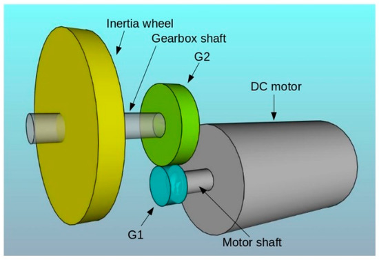
Figure 1.
Components of the system to be controlled.
Due to this, it is necessary to add Equation (5) (Equation (2) modified) and Equation (6), which are inspired by the guidelines outlined in [15].
Now, in Equation (5), J1 is the moment of inertia of the motor shaft, w1 its angular velocity, fv1 its viscous friction, F is the tangential force generated at the edge of the gear coupled to the motor shaft, RG1 is the radius of the gear coupled to the motor shaft, and finally, τ1 is the torque generated by the DC motor (Figure 2).
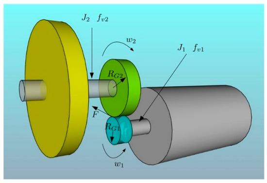
Figure 2.
Parameters and variables of the system.
In Equation (6), F is the tangential force that is exerted on the edge of the gear coupled to the output shaft (in contact with the gear of the motor shaft). In fact, it is the force exerted by the motor on the edge of the gear coupled to its axis. RG2 is the radius of the gear coupled to the output shaft (of the reduction stage), fv2 is the viscous friction, w2 is the angular velocity (of the reduction stage), and finally, J2 is the moment of inertia of the gearbox shaft, which also includes the moment of inertia of the flywheel.
Calling η the relation and considering that , we finally obtain Equation (7) by solving Equations (5) and (6), taking advantage of the fact that the two share the variable F.
To obtain the speed of the output shaft, according to the applied torque, proceed as follows, approximating the derivatives by backward differences:
Now a complete motor simulator can be programmed, with Equation (10) and Equations (1)–(4) to obtain τ1(n), which finally allows us to obtain the angular velocity of the shaft output of the motor gearbox shaft, from the evolution in the motor’s input voltage (again the derivatives of Equations (1) and (2) have been approximated by backward differences).
The parameters used in the experiments carried out are mainly those corresponding to a commercial 24 v/70 W brush engine from a prestigious manufacturer:
- R: 1.11 Ω → resistance of the rotor winding
- L: 0.0002 H → self-inductance
- K: 0.0634 Nm/A → constant of proportionality
- J1: 6.77 * 10−6 Kg∙m2 → the moment of inertia of the motor shaft
- J2: 9.1 * 10−7 Kg∙m2 + moment of inertia of the wheel → moment of inertia of the gearbox shaft
- η: 26:1 → gearbox relation
With this configuration and the model, it is possible to calculate the energy consumed in response to a step setpoint change, following Equation (11), expressed in kilowatts per second. Note that this parameter can be positive or negative in function of whether the motor works as a motor or as a generator. In that second case, it is considered recovered energy.
Finally, it is necessary to emphasize that the period T, for each simulation cycle, has been determined considering the bandwidth of the system (BW), to respect the sampling theorem of [16,17]. In this theorem, an upper limit T ≤ 1/(2 BW) is imposed, to avoid “aliasing” problems in sampled systems.
The bandwidth of the system changes depending on the flywheel used in the tests, as shown in Table 2.
Table 2.
Required system bandwidth.
3. PID Controllers and Performance Indexes
Possibly one of the best references for introducing PID controllers is [18]. It establishes that PID controllers constitute a major advance compared to all-or-nothing (on-off) controllers.
The simplest configuration, a proportional-only controller, reduces the oscillation due to the overreaction of the on-off controllers. The response is proportional to the currently detected error. However, proportional controllers have the disadvantage that, depending on the type of system to be controlled, they cannot eliminate the steady-state error.
To solve this situation, the integral control alternative appears. In this case, a correction is introduced in the controller output proportional to the integral of the error, which is calculated from the beginning of the system’s operation up to the present moment. The integral component increases the type of system, which helps eliminate the steady-state error. The disadvantage of the integral contribution is that it is easy to generate unstable behaviors that prevent reaching a suitable steady-state.
An added improvement consists of anticipating the behavior of the error by estimating it, which allows activation of a “forward-looking” correction. That is what the derivative contribution achieves, which is proportional to the derivative of the error.
A controller with the three components mentioned (Proportional, Integral, and Derivative) is called a PID. In [18], it is stated that more than 95% of industrial control problems are solved with PID controllers, although most of them are only PI.
The performance of a PID controller is usually estimated based on the application for which it was designed. However, there are a series of performance indexes that allow the correctness of its operation to be determined, as well as an assessment of the choice of gains and parameters selected for its implementation. These parameters are evaluated based on a step-response setpoint of the PID controller and allow its gains to be adjusted and its optimization.
The most widely used performance indexes are settling time, decay ratio, overshoot, and steady-state error for step changes in a setpoint response. These indexes are defined next, considering the description of Aström [18].
- Settling time (tss): Time it takes for the system to reach p% of the steady-state value in response to a step-response. The default value of p, in most cases, is 2%.
- Decay ratio (d): Ratio between two consecutive maxima of the error for a step change in setpoint. A quarter amplitude damping (d = l/4) is used as default.
- Overshoot (o): Ratio between the difference between the first peak of the system response and the steady-state value of a step change in setpoint. An acceptable value of o is within the interval (8–10%). However, in function of the application, an overdamped response with no overshoot can be desirable.
- Steady-state error (ess): Value of the difference between the system response, once stabilized, and the setpoint.
Multiple approaches are followed to design controllers in general and PIDs. In the case of PID controllers, there are some very frequently used alternatives, such as the root-place method [19] or the Ziegler-Nichols method [20]. However, although the use of these methods generates solutions with adequate behavior in the action range, in no case is it guaranteed that the defined parameters generate optimal behavior. Consequently, when it is necessary to optimize this kind of controllers, an additional optimization technique must be applied.
In this specific case, the presented controller whose parameters are going to be optimized is a speed controller, whose control architecture as well as the relations with the optimization mechanisms is defined in Figure 3.
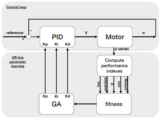
Figure 3.
Block diagram that represents the control loop and que optimization procedure.
4. Optimization with Metaheuristics
This paper uses Evolutionary Computation for the optimization process as will be explained in Section 4.2. Specifically, the balance between motor performance indexes and energy consumption is the relationship optimized through genetic algorithms. The motor performance indexes have been optimized considering the energy consumption, obtaining as a result the best values for the PID parameters.
4.1. Definition of the Objective Function
Every optimization problem consists of the maximization or minimization of an objective function subject to a series of restrictions. Both the objective function and the constraints are dependent aspects of the problem, while general-purpose processes of searching for a maximum or a minimum are used and can therefore be applied to any well-defined problem. For this reason, it is necessary to define the function to be optimized prior to any optimization.
Optimal control deals with the problem of finding a control law for a given system so that a certain optimality criterion is achieved. A control problem includes a cost function involving state and control variables.
In the case of the problem presented in this paper, the optimization will be carried out on a sequence of 30 randomly-generated control instructions. The controller should reach the first setpoint, then the second, etc. This sequence of instructions, although random, will remain constant for all experiments, although subsequent validation with new instructions will be carried out in a cross-evaluation process.
For the optimization process, we will start from the metric described in [9], which includes the combination of four system performance measures (tss, overshoot, dy, ess) combined linearly applying four alpha, beta, gamma, and delta weights, which are shown in Table 3. Those weights are an empirical approximation, but they can be modified to enhance a certain behavior, when required. For example, in the event of minimization of the settling time, even at the expense of other parameters, it is possible to increase the alpha parameter, and the same for the other components. This process is graphically shown in Figure 3, including the control architecture.
Table 3.
Weights assigned to each regulator performance index.
We have added an additional component to this metric, which is the energy consumed to complete each setpoint. This measure will be combined with the previous components using a percentage coefficient of participation in the global metric. To calculate the weight ε to be used based on the desired participation percentage, Equation (12) is applied.
where We is the weight of energy in the calculation of fitness and represents the percentage of importance that you want to give to energy.
Therefore, the equation of the system’s error for a sequence of pulses will be defined as Equation (13), for a series of steps S.
Finally, the fitness function to be used by the metaheuristics is defined in Equation (14).
The objective of this optimization problem is defined as the maximization of Equation (14), subject to the values of the gains of the PID controller (Kp, Ki, Kd) ∊ [0, 100], following the sequence of block diagram of Figure 3.
This optimization is transparent to the plant that supports the optimization, simulated (as in this case) or real. The addition of hardware-in-the-loop in the tuning process is a challenging topic in the control area. To tune real DC drives with the proposed method we should substitute the call to the model in each control loop cycle by calls to the drive, reading the real angular speed, only considering the inherent physical restrictions and limitations. The setup of this tuning should be made in two steps: (i) Tune without load; (ii) fine tune in load situations, with limited setpoints.
4.2. Definition of the Architecture of Genetic Algorithms
Optimization has been performed using evolutionary computation based on real number chromosomes. In our case, the selected chromosome length is 3 to represent the three parameters of a PID controller (Kp, Ki, and Kd), which are the variables to be optimized to achieve the highest possible fitness. With the given definition of fitness, the maximum possible value is 1, which would correspond to an error = 0.
As operators, we will use the following. For the selection, we will use tournament with T = 6 [21]. For the crossover operator we will use BLX-alpha [22] and for the mutation operator we will use Gaussian jump with mean 0 and initial standard deviation equal to ¼ of the maximum range of the parameter [23]. The standard deviation of the Gaussian leap will decrease over generations by a factor of 0.999, following a simulated tempering scheme. The remaining parameters of the genetic algorithm are, population size = 100 individuals, mutation rate = 0.33 (1/3 of the chromosome size), and crossover rate = 0.7.
5. Testing
As an experiment we have selected two concrete instances of the motor simulator defined in Section 2, operating on an inertia wheel.
The use of the inertia wheel is necessary to bring the DC motor closer to real world situations by introducing a workload. An inertia wheel is usually dimensioned (mass, radius, and height) to introduce a moment of inertia added to a rotating system that can be used in this case to simulate the system that has to be moved.
With the flywheel, we obtain an additional important benefit, which is the reduction of the system’s bandwidth. Its sampling frequency can thus be lower and, ultimately, the presented controller can be activated at a lower frequency.
To test the response of the proposed system, two cases are defined, depending on the size of the inertia wheel, which implies a significant variability of the system behavior.
- Case 1: With a 500 g flywheel and 20 cm radius.
- Case 2: With a 5 kg flywheel and a 10 cm radius.
For both cases, the sampling frequency will be 0.1 Hz, since it is within the theoretical range calculated in Table 2.
For each case, the optimization process has been carried out in various scenarios with respect to the relative importance of energy consumption, from 0% (consumption is not considered), to 50% (consumption is the most important). The values chosen for each instance of the motor are different since, depending on the weight of the flywheel and its radius, the energy necessary to move it with a certain acceleration varies significantly. Therefore, the weight given to the relationship must be higher when the flywheel is lighter if we want the effect to be more noticeable in the control signal. However, any change in weight has consequences when measuring consumption: The higher the weight for the energy component, the lower the energy consumption, and vice versa.
For all experiments, 50 generations of the evolutionary algorithm were performed, using a tournament selection with T = 6. Each generation takes an average time of 2.55 s, therefore, the total time for each optimization is around 127.5 s. These parameters are considered adequate and sufficient to achieve optimization.
The mutation probability is usually chosen as 1/L, where L is the length of the chromosome for a gene to mutate on average in each individual and generation [24]. The matching probability does not have much of an impact if it is high enough (close to 1). The T parameter of the tournament selection indicates the position in the exploration/exploitation dilemma. Low values give preference to exploration, that is, searching in many different points of the problem space, and high values give preference to exploitation, or rather, improving solutions already found. An excessive preference for exploitation produces a very rapid convergence (in a few generations) but might easily fall to local minima. An excessive preference for exploration avoids local minima but might not sufficiently favor the best solutions, and therefore, becomes a mere random search for the solution, having an excessively slow convergence or even no convergence at all. For this problem, the best results have been found with T = 6, that is, a sufficiently fast convergence is obtained without easily falling to local minimums.
The number of generations has been set at 50 because this value offers a good solution convergence in all tested cases.
5.1. Results
The results of the tests carried out are shown in Table 4, where Kp, Ki, Kd are the PID controller parameters, training error is the global error calculated with the proposed metric on the adjustment sequence, and test error is the global error calculated with the proposed metric on the test sequence. No-energy test sequence error is the total error on the test sequence without taking energy into account, that is, it merely measures the performance of the controller without regarding its efficiency. Energy used is that consumed in the adjustment sequence, while energy recovered is the energy recovered in the form of negative voltage. This energy parameter represents the energy consumed by the electric motor in the event of a step response setpoint as expressed in Equation (11). We is the weight of the energy in the fitness definition as expressed in Equation (12).
Table 4.
Results of the optimization tests for the two cases defined.
Finally, the average stabilization time is the average system response time, which is used to show a view of the relationship between performance and energy consumption.
In Tables 4 and 6, tests are presented for each case with different We, between 0% and 50%, and between 0% and 5% for case 2.
To compare the results of the control, we should ignore the contribution of energy to the error. To do this, the parameter “no-energy test error” has been calculated. This represents the error of Equation (12) excluding the participation of energy. In other words, energy has been used to adjust the parameters, but now we look at how the controller behaves in other aspects (tss, d, overshoot, and ess), since energy saving logically degrades the behavior of the system in other parameters, especially in the tss.
In Table 4, as the importance of efficiency is increased, the performance of the controller decreases. This is logical because with smoother accelerations the applied voltage is lower. However, it also takes longer to reach the setpoint, which is one of the parameters used to measure the performance of the controller. Consumption is seen to be reduced by more than an order of magnitude as we increase its weight in the fitness of the evolutionary algorithm. On the other hand, we see that by giving more weight to energy efficiency, the controller adjusts so that more energy is recovered. A gradual transition as the weight of consumption is increased is also observed, although the percentages of influence that must be applied are highly dependent on the configuration of the engine and inertia wheel. This can be seen in case 1, where with a weight of 5% the maximum efficiency is reached, while in problem 2 a weight of 50% was needed to reach maximum efficiency.
5.2. Results of the Bootstrapping Estimation
For an accurate estimation of the results obtained and their tolerance to changes in the instructions, the bootstrapping technique [25] has been used. This technique is based on resampling the problem space N times and calculating the parameter values for each sample. Finally, by organizing the results and discarding a certain percentage of the samples at each end of the sequence, we obtain a confidence interval for each parameter. Bootstrap error estimation is much more reliable than traditional cross-evaluation estimation because it avoids the limitation of working with a single randomly chosen test set, since excessively optimistic or pessimistic results can be obtained depending on which set is selected. The bootstrap guarantees that the estimated parameter is within a previously established range of significance, making it possible to obtain not only a much more reliable estimate of the parameter than the cross-evaluation, but also a confidence interval for that parameter.
For example, if we want to obtain the 95% confidence interval of the error produced by a set of PID parameters, we will take the Kp, Ki, Kd values and use them to measure the error made (using the metric defined in Section 4.1) during a randomly generated sequence. This process will be repeated N times (10,000, in our case, which means calculating the error for 30 steps × 10,000 trials = 300,000 setpoints). The result of the process will be 10,000 error values, with which we will obtain the estimate of the expected error by averaging these values. On the other hand, if we organize the errors from smallest to largest and take one at position 250 and another at position 9750, we will obtain the 95% confidence interval of the error that the system will produce in any real situation.
The same procedure has been used to estimate the confidence intervals of the energy consumed per route and the energy recovered, observing that the variation of these is greater because each sequence presents different energy requirements and their setpoints are different.
It is possible to use any N with any confidential level p, calculating the number of D values to discard for each side, once organized, using Equation (15).
Table 5 shows the verification of the experimental results of the optimization obtained by applying the genetic algorithms, obtaining the improved values for parameters Kp, Ki, and Kd. The columns in the table are as follows: Kp, Ki, Kd: PID controller parameters prototypes once optimized; the remaining columns represent the results of the bootstrap experiments for those optimized parameters; We: Weight of consumption in the fitness function; Test error: Mean error obtained with the proposed metric for the 10,000 randomized trials; Energy: Average energy consumed in the 10,000 tests; Recovered: Average energy recovered in the 10,000 tests. Confidence interval: Confidence level at 95% of the three estimated parameters.
Table 5.
Results of the optimization tests for the two selected cases using bootstrap.
Table 5 shows that the error remains limited to low values despite the enormous variability of the tests generated, which validates the stability of the proposed controller for practically any operating situation. In the case of energy and recovery, the variability is greater, which is logical because, as the sequences are randomly generated, their energy requirements vary greatly. A sequence with small speed variations is not the same one with very large ones.
From all the cases analyzed in Table 5, three tests from case 2 have been selected to graphically show the performance of the controllers. Those tests give a detailed description of the transition from increasingly demanding configurations with respect to the energy consumed. They represent the optimized controllers obtained for energy weights of 0%, 2%, and 4%. Figure 4, Figure 5 and Figure 6 show the outputs of the control performed by each controller, the energy consumed, and the accelerations. These figures have three axes, (a), (b) and (c). In Figure 4a, Figure 5a and Figure 6a, the angular speed of the motor is shown, together with the sequence of step by step instructions to which the control system is subjected, in Figure 4b, Figure 5b and Figure 6b, the energy consumed in kilowatt-second (kws) obtained in response to those cases, and in Figure 4c, Figure 5c and Figure 6c, motor acceleration in rad/sec2 for those same cases. The x-axis shows the time in seconds from the start of the sequence.
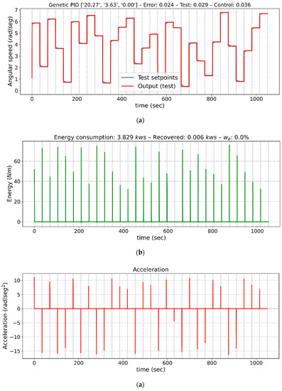
Figure 4.
Graphs of controller outputs, instantaneous energy consumed, and acceleration for the proportional-integral-derivative (PID) adjusted with an energy weight of 0%, that is, without considering consumption. (a) Speed response of the drive, (b) Energy consumption, (c) Acceleration of the drive.
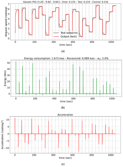
Figure 5.
Graphs of controller outputs, instantaneous energy consumed, and acceleration for the adjusted PID with a 2% energy weight. (a) Speed response of the drive, (b) Energy consumption, (c) Acceleration of the drive.
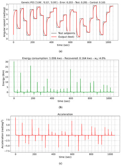
Figure 6.
Graphs of controller outputs, instantaneous energy consumed, and acceleration for the adjusted PID with a 4% energy weight. (a) Speed response of the drive, (b) Energy consumption, (c) Acceleration of the drive.
Figure 4 shows the behavior of the controller with a weight of 0% for the consumed energy component. It also shows that the response to the different instructions is immediate, but energy consumption is very high. Specifically, the average stabilization time is 1.67 s and average consumption is 20.78 kw/s. This is logical, because optimization of the control parameters seeks to improve performance as much as possible regardless of the cost of energy. No overshoot, steady-state errors, or oscillatory behaviors are observed.
Figure 5 shows the behavior of the controller with a weight of 2% for the consumed energy component. In this case, the graph shows that the response to the step command is a little slower than in the previous case, with a lower speed slope, which results in a longer stabilization time. No overshoot, steady-state errors, or oscillatory behaviors are observed. However, the weight of 2% in Equation (12) implies that the average energy consumption is 53.14% lower than in the previous case, while the average stabilization time has risen by 9.30 s.
Finally, Figure 6 shows the behavior of the controller with a weight of 4% for the consumed energy component. For this third selected case, the graph shows that the response to the step command is slightly slower than in the two previous cases, with a lower speed slope, which results in a longer stabilization time. No overshoot, steady-state errors or oscillatory behaviors are observed. However, the weight of 4% in Equation (12) implies that the average energy consumption is 66.38% lower than in the previous case, while the average stabilization time has risen by 0.7 s.
The differences between the different cases are very large, both in terms of stabilization time and energy consumption. This means that there is no single optimization, as it will depend on the application where the controller is to be used. Therefore, depending on this application, a configuration should be sought where performance and energy consumption are adequately balanced. Thus, there will be applications in which performance is critical, regardless of energy consumption, and others whose demand is the opposite, so extreme values such as those shown in the previous figures are perfectly valid. The design of the planned optimization system allows this functionality, by selecting the optimization parameters based on the behavior of the desired system, supporting multiple control regimes with an on-demand application.
6. Conclusions
This paper presents a PID controller optimization method for direct current motors with an inertia wheel that takes consumption into account. Our system finds optimal control parameters to adjust controller gains and achieve good behavior in terms of tss, d, overshoot, and ess, also considering the motor’s energy savings. Our system allows us to assign a percentage for the importance of energy saving compared to the smooth performance of the controller.
As the weight of the energy increases, more efficient controllers are obtained although at the cost of poorer performance in terms of tss, d, overshoot, and ess, even though it is important to mention that there are also controllers with great energy savings and an insignificant loss of performance. However, the relative importance that we must assign to energy consumption differs greatly from one motor to another, so a specific study is necessary for each real motor.
Our studies on simulated motors show that a 60% saving is possible by slightly influencing the performance indexes, especially the ess and stabilization time. However, the system allows us to adjust the optimization parameters and to achieve a balanced behavior between performance and energy consumption for each application.
Author Contributions
F.S. oversaw the implementation of the optimization algorithms and testing; N.C. was responsible for defining the controller and model; J.E.N. was in charge of the coordination of the presented works. All authors have read and agreed to the published version of the manuscript.
Funding
This research was funded by Programa Estatal de Investigación, Desarrollo e Innovación Orientada a los Retos de la Sociedad PID2019-104793RB-C33 and Region of Madrid Excellence Network SEGVAUTO 4.0.
Conflicts of Interest
The authors declare no conflict of interest.
References
- Pontryagin, L.S.; Boltyanskii, V.G.; Gamkrelidze, R.V.; Mishchenko, E.F. The Mathematical Theory of Optimal Processes; Interscience: Saint Nom, France, 1962; (Original in Russian, cited in English Translation). [Google Scholar]
- Geering, H.P. Optimal Control with Engineering Applications; Springer: Berlin/Heidelberg, Germany, 2007. [Google Scholar]
- Sieniutycz, S. Hamilton–Jacobi–Bellman equations and dynamic programming for power-maximizing relaxation of radiation. Int. J. Heat Mass Transf. 2007, 50, 2714–2732. [Google Scholar] [CrossRef]
- Hayashi, Y.; Hanai, Y.; Matsuki, J.; Fuwa, Y.; Mori, K. Determination of the optimal control parameters of voltage regulators installed in a radial distribution network. IEEJ Trans. Electr. Electron. Eng. 2008, 3, 515–523. [Google Scholar] [CrossRef]
- Wang, H.; Zhou, H.; Wang, D.; Wen, S. Optimization of LQR controller for inverted pendulum system with artificial bee colony algorithm. In Proceedings of the 2013 International Conference on Advanced Mechatronic Systems, Luoyang, China, 25–27 September 2013; pp. 158–162. [Google Scholar]
- Mora, L.; Lugo, R.; Amaya, J.E.; Moreno, C. Parameters optimization of PID controllers using metaheuristics with physical implementation. In Proceedings of the 35th International Conference of the Chilean Computer Science Society (SCCC 2016), Valparaiso, Chile, 10–14 October 2016; pp. 1–8. [Google Scholar]
- Puchta, E.D.P.; Siqueira, H.V.; Kaster, M.D.S. Optimization Tools Based on Metaheuristics for Performance Enhancement in a Gaussian Adaptive PID Controller. IEEE Trans Cybern. 2020, 50, 1185–1194. [Google Scholar] [CrossRef] [PubMed]
- Rodríguez-Molina, A.; Mezura-Montes, E.; Villarreal-Cervantes, M.G.; Aldape-Pérez, M. Multi-objective meta-heuristic optimization in intelligent control: A survey on the controller tuning problem. Appl. Soft Comp. 2020, 93, 106342. [Google Scholar] [CrossRef]
- Naranjo, J.E.; Serradilla, F.; Nashashibi, F. Speed Control Optimization for Autonomous Vehicles with Metaheuristics. Electronics 2020, 9, 551. [Google Scholar] [CrossRef]
- Yang, X.S. Engineering Optimization: An Introduction with Metaheuristic Applications; John Wiley & Sons: Hoboken, NJ, USA, 2010. [Google Scholar]
- Lessmann, S.; Caserta, M.; Arango, I.M. Tuning metaheuristics: A data mining based approach for particle swarm optimization. Expert Syst. Appl. 2011, 38, 12826–12838. [Google Scholar] [CrossRef]
- Dobslaw, F. A parameter tuning framework for metaheuristics based on design of experiments and artificial neural networks. In Proceedings of the International Conference on Computer Mathematics and Natural Computing, Rome, Italy, 28 April 2010; Brojack, B., Ed.; WASET: Paris, France, 2010. [Google Scholar]
- Huang, C.; Li, Y.; Yao, X. A Survey of Automatic Parameter Tuning Methods for Metaheuristics. IEEE Trans. Evol. Comp. 2020, 24, 201–216. [Google Scholar] [CrossRef]
- de Silva, C.W. Modeling and Control of Engineering Systems; CRC Press: Boca Raton, FL, USA, 2009; Chapter 4.5.2. [Google Scholar]
- Burns, R.S. Advanced Control Engineering; Buterworth Heinemann: Woburn, MA, USA, 2001; Chapter 2.4.3. [Google Scholar]
- Fadali, M.S.; Visioli, A. Digital Control Engineering. Analysis and Design; Prentice Hall: Upper Saddle River, NJ, USA, 2009; Chapter 2.9. [Google Scholar]
- Orfanidis, J. Digital Signal Processing; Horwood Publishing: Sawston, Cambridge, UK, 2010; Chapter 1.3. [Google Scholar]
- Aström, K.J.; Murray, R.M. Feedback Systems. An Introduction for Scientist and Engineers, 2nd ed.; Princeton University Press: Princeton, NJ, USA, 2019; Chapter 1.5. [Google Scholar]
- Nise, N.S. Control Systems Engineering; John Wiley and Sons: Street Hoboken, NJ, USA, 2011; Chapter 9. [Google Scholar]
- Ogata, K. Modern Control Engineering; Prentice Hall: Upper Saddle River, NJ, USA, 2010; Chapter 8.2. [Google Scholar]
- Takenouchi, H.; Tokumaru, M.; Muranaka, N. Performance evaluation of interactive evolutionary computation with tournament-style evaluation. In Proceedings of the 2012 IEEE Congress on Evolutionary Computation, Brisbane, Australia, 10–15 June 2012; pp. 1–8. [Google Scholar]
- Herrera, F.; Lozano, M.; Sánchez, A.M. A taxonomy for the Crossover Operator for Real-Coded Genetic Algorithms: An Experimental Study. Int. J. Intell. Syst. 2003, 18, 309–338. [Google Scholar] [CrossRef]
- Guo, J.; Wu, Y.; Xie, W.; Jiang, S. Triangular Gaussian mutation to differential evolution. Soft Comput. 2020, 24, 9307–9320. [Google Scholar] [CrossRef]
- Jansen, T.; Wegener, I. On the Choice of the Mutation Probability for the (1+1) EA. In Parallel Problem Solving from Nature; Springer: Berlin/Heidelberg, Germany, 2000. [Google Scholar]
- Mouret, J.-B.; Doncieux, S. Overcoming the bootstrap problem in evolutionary robotics using behavioral diversity. In Proceedings of the 11th IEEE Congress on Evolutionary Computation (CEC’09), Trondheim, Norway, 18–21 May 2009; pp. 1161–1168. [Google Scholar]


Publisher’s Note: MDPI stays neutral with regard to jurisdictional claims in published maps and institutional affiliations. |
© 2020 by the authors. Licensee MDPI, Basel, Switzerland. This article is an open access article distributed under the terms and conditions of the Creative Commons Attribution (CC BY) license (http://creativecommons.org/licenses/by/4.0/).