Abstract
This work presents an analytical series-form solution for the time-harmonic electromagnetic (EM) field components produced by an overhead current line source. The solution arises from casting the integral term of the complete representation for the generated axial electric field into a form where the non-analytic part of the integrand is expanded into a power series of the vertical propagation coefficient in the air space. This makes it possible to express the electric field as a sum of derivatives of the Sommerfeld integral describing the primary field, whose explicit form is known. As a result, the electric field is given as a sum of cylindrical Hankel functions, with coefficients depending on the position of the field point relative to the line source and its ideal image. Analogous explicit expressions for the magnetic field components are obtained by applying Faraday’s law. The results from numerical simulations show that the derived analytical solution offers advantages in terms of time cost with respect to conventional numerical schemes used for computing Sommerfeld-type integrals.
1. Introduction
The computation of the electromagnetic (EM) fields from overhead electric lines located above dissipative terrestrial areas is a classical problem which is still of interest today because of the public concern about the biological effects of field exposure. In fact, it is well known that the strong EM fields associated with the high-intensity currents and voltages of power lines can generate undesirable effects on humans, animals and other forms of life [1,2,3]. The problem, in all of its variants, has spawned a number of contributions to the scientific literature since a solution was first developed at the beginning of the 20th century by Carson [1,2,3,4,5,6,7,8,9,10,11,12,13,14,15,16,17,18,19,20,21,22,23,24,25]. Yet, in spite of the variety of proposed approaches, to Author’s knowledge there is scarcity of purely analytical techniques in literature, and most of the published methods attempt to solve the problem through the derivation of analytical formulations amenable to numerical treatment. Excellent illustrations of these approaches are the well-known method of moments (MoM), which is used to solve surface integral formulations, and the method of auxiliary sources [10], consisting of expressing the fields as weighted superpositions of the contributions from a finite number of fictitious currents flowing on mathematical surfaces separated from the air-ground interface. Even if these methods may exhibit good performances in terms of accuracy and efficiency, as numerical procedures they suffer from the intrinsic disadvantage of involving memory requirements and computational costs significantly greater than those implied by an analytical solution. Moreover, they provide less insight in the physics of the problem and are also less suitable for sensitivity analysis. On the other hand, one important contribution in the context of purely analytical techniques is the work by Prof. J. R. Wait [5], which presents field expressions derived through usage of the complex image theory. The only drawback of the obtained formulas resides in that they are valid in the quasi-static regime only, that is when the effects of the displacement currents in the air space are negligible. The aim of the present paper is to derive rigorous series-form expressions for the time-harmonic EM field components produced in the air-space by a uniform-current line source located above a homogeneous dissipative ground. The field expressions are obtained starting from decomposing the integral representation for the axial component of the generated electric field into three parts, that is the direct field induced by the source current, the ideal reflected field induced by a negative image current and a correction term due to the imperfect conductivity of the ground. Next, after recognizing that the first two terms can be straightforwardly expressed in explicit form, the non-analytic part of the integrand of the correction term is expanded into a power series of the vertical propagation coefficient in the air space. This permits to express the electric field as a sum of derivatives of the Sommerfeld Integral describing the direct field. As a result, the field is given as a sum of cylindrical Hankel functions, with coefficients depending on the position of the field point relative to the original current source and its ideal image. Finally, analogous explicit expressions for the magnetic field components are obtained by applying Faraday’s law. The obtained solution is not subject to simplifying assumptions, and hence is valid even when the high-frequency effects due to the displacement currents in both the air and the soil are not negligible. As a consequence, the solution is also of practical use as an analytical benchmark for simulation tools employed to solve EM boundary value problems. Numerical tests are performed to show the validity of the developed method and its advantages in terms of computation time with respect to standard numerical algorithms used to evaluate Sommerfeld-type integrals.
2. Formulation of the Problem
Consider an infinite line source of current located in proximity of a flat homogeneous ground, as shown in Figure 1.
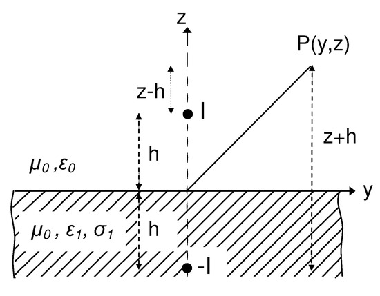
Figure 1.
Sketch of a line source of current above a homogeneous ground.
The line is situated above the ground at height h, and the material medium is characterized by the dielectric permittivity and electrical conductivity , while the magnetic permeability is taken to be everywhere that of free-space . Under the hypothesis that the observation point lies in the near-field region of the line source, it is reasonable to assume that the line supports a nearly uniform current [1], i.e., . Due to the symmetry of the problem, the total electric field generated in the air space has only one component in the axial direction, whose integral representation is well known and given by [10]
where
and
are, respectively, the Sommerfeld Integrals describing the direct and reflected fields, being the zeroth-order Hankel function of the second kind, and . The aim of this paper is to derive exact series representations for and the magnetic field components, the latter arising from applying Faraday’s law. To this goal, it is first convenient to use the identity
and split into two terms, that is the ideal reflected field contribution (induced by a negative image current) plus a term due to the imperfect conductivity of the ground. It reads
with
and where account has been taken of (2). The integral may be evaluated by proceeding as follows. After setting and
we replace the quantity , where is a non-negative real constant to be determined, with its Taylor expansion about = 0, in a similar fashion as in [5]. It yields
and, as a consequence, (6) becomes
being = . Under the assumption that > 0, the second integral on the right-hand side of (9) converges regardless of the value chosen for the non-negative arbitrary constant . This happens because, as becomes sufficiently large, the exponential factor approaches , which rapidly decays with increasing . Since may be assumed to be as small as desired, we now take the limit of (9) as . It is not difficult to prove that, subject to this condition, the odd coefficients () become null. On the other hand, the limit of the even coefficients reads
and, as a consequence, (9) may be expressed as
where the -derivatives of , that is the derivatives of , are to be made explicit. After letting let r = , from the differential properties of the Bessel functions [26] it follows that
where the argument of the Hankel functions, that is , has been omitted for notational simplicity, and with
It should be noted that the number of terms on the right-hand sides of (12) is for even l, and for odd l. Hence, it is equal to unity plus the integer part of , denoted by . Next, use of the tabulated result [26]
into (12) leads to the expression
and
Finally, substituting (2) and (15) into (11) provides
with
and hence, the total axial electric field component (1) may be rewritten as
The non-null magnetic field components may be obtained from by applying Faraday’s law, as follows
In fact, differentiating (17) with respect to leads to write
and, as a consequence, (20) is turned into
On the other hand, since it holds
and, therefore,
the explicit expression for the -field reads
3. Results
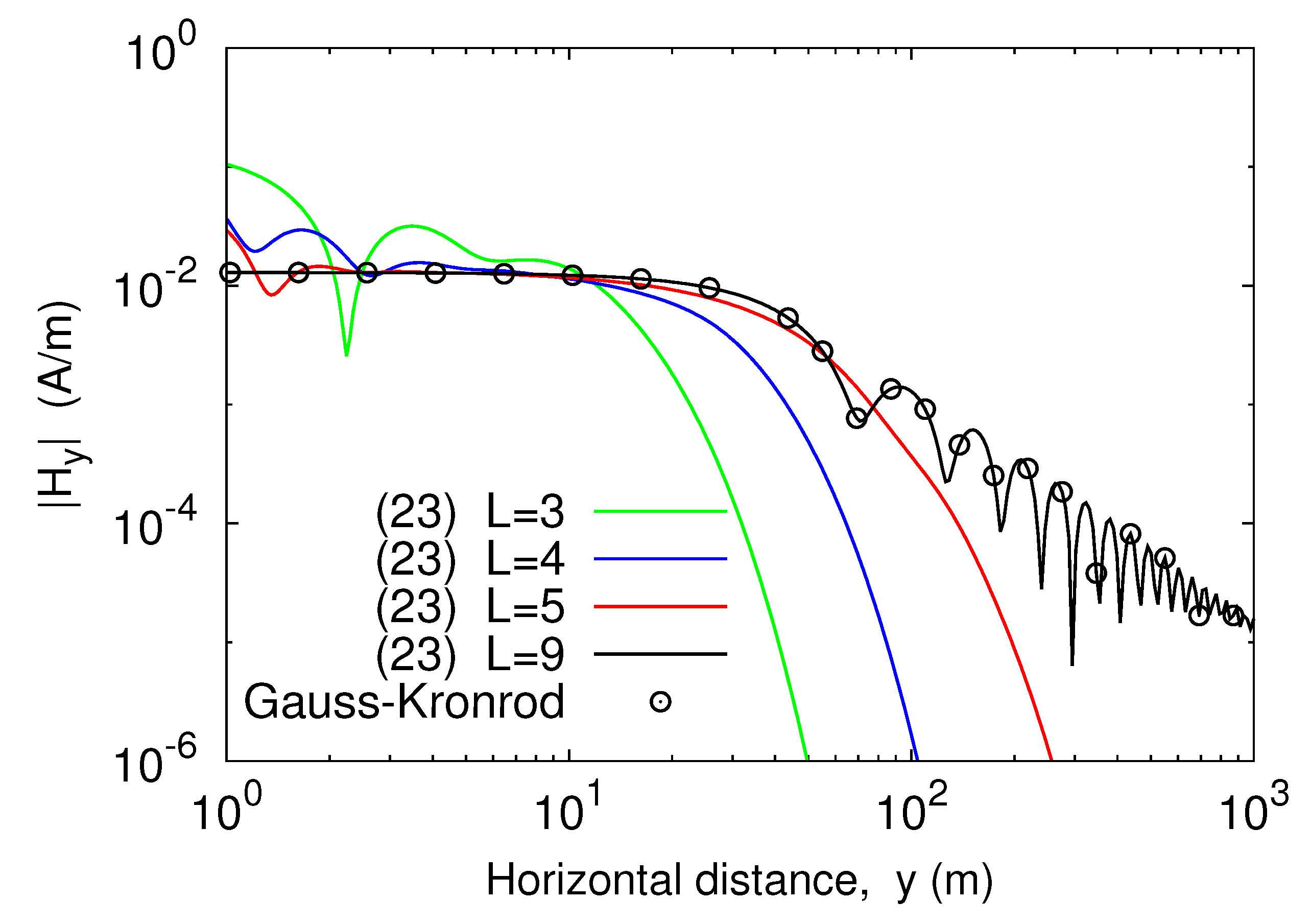
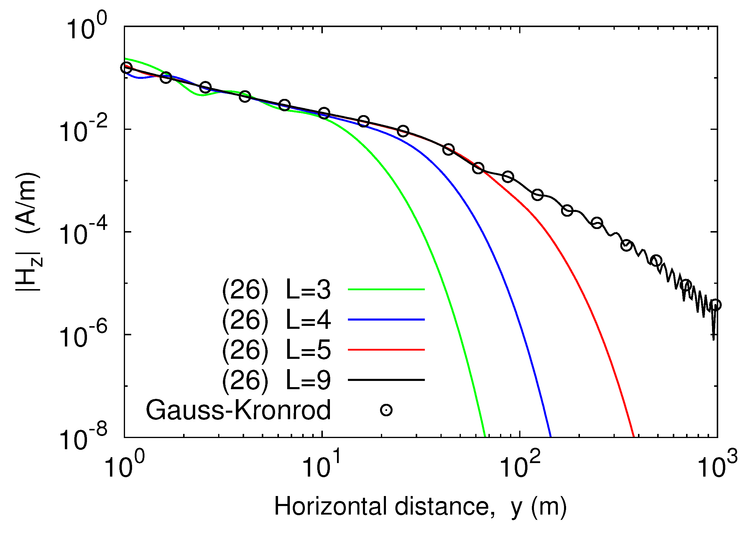
As validation of the theoretical development, expressions (23) and (26) were used to calculate the magnetic field components that an infinite line source carrying 1 A of current produced at a plane 1 m above the interface between air and a clay soil. The source was situated 4 m above the material medium, whose electrical conductivity and dielectric permittivity were taken to be equal to = 0.1 mS/m and = 40 , respectively [27]. At first, the fields were computed against the horizontal distance y from the line axis, assuming that the operating frequency was equal to 1 MHz. Four y-profiles were generated, each one corresponding to a different value for the truncation index L of the outer infinite sum in (18). The results of the computations, shown in Figure 2 and Figure 3, were compared with those arising from numerically evaluating the integral representations for the magnetic field components, namely [28]
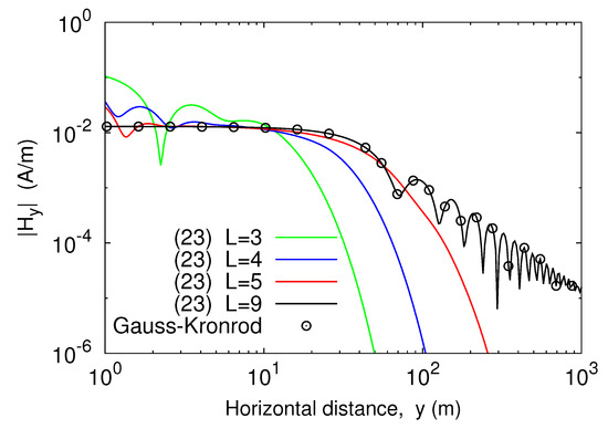
Figure 2.
Amplitude of against the horizontal distance from the line source.
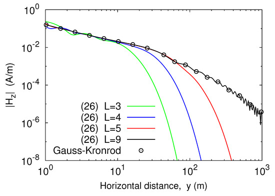
Figure 3.
Amplitude of against the horizontal distance from the line source.
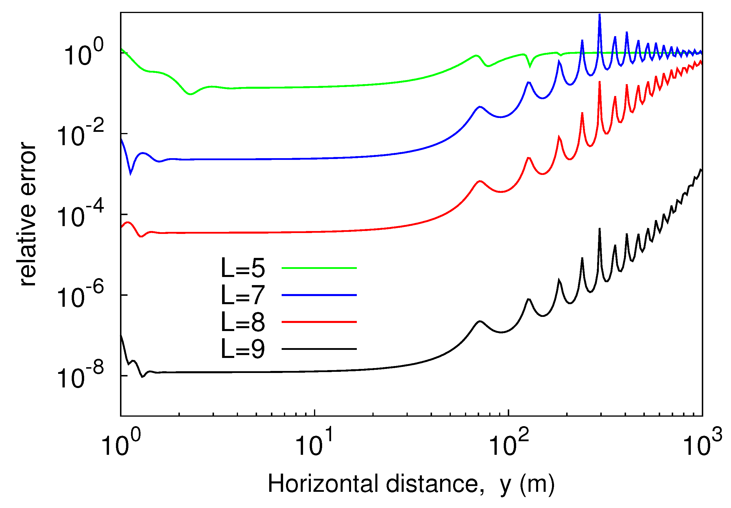
Numerical integration was carried out by applying a Gauss–Kronrod G7-K15 scheme, originating from the combination of a seven-point Gauss rule with a 15-point Kronrod rule. From the analysis of the plotted curves it emerged that increasing the truncation index L improved the accuracy of the result of the computation. In fact, if L grew the curves provided by (23) and (26) approached the outcomes from numerical quadrature, and close agreement was achieved when L = 9 in both the situations. Thus, the proposed series-form solution converged to the exact solution. This was confirmed by the curves plotted in Figure 4, which show the relative error of the outcomes from (23) as compared to numerical integration data. As is seen, the error monotonically decreased as L increased. On the other hand, for a fixed value of L the error was not substantially affected by a variation of the distance y as long as the latter was smaller than 50 m. Thereafter, the relative error grew and exhibited an oscillating behavior, pretty similar for all the considered values of the truncation index of the outer sum in (18). However, even with the rapid increase as the distance y increased, for the error did not exceed in the considered interval.
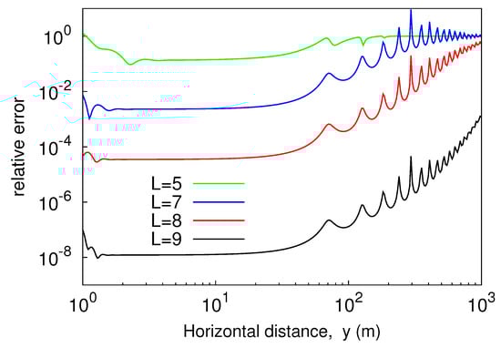
Figure 4.
Relative error of (23) as compared to G7-K15 scheme, plotted versus y.
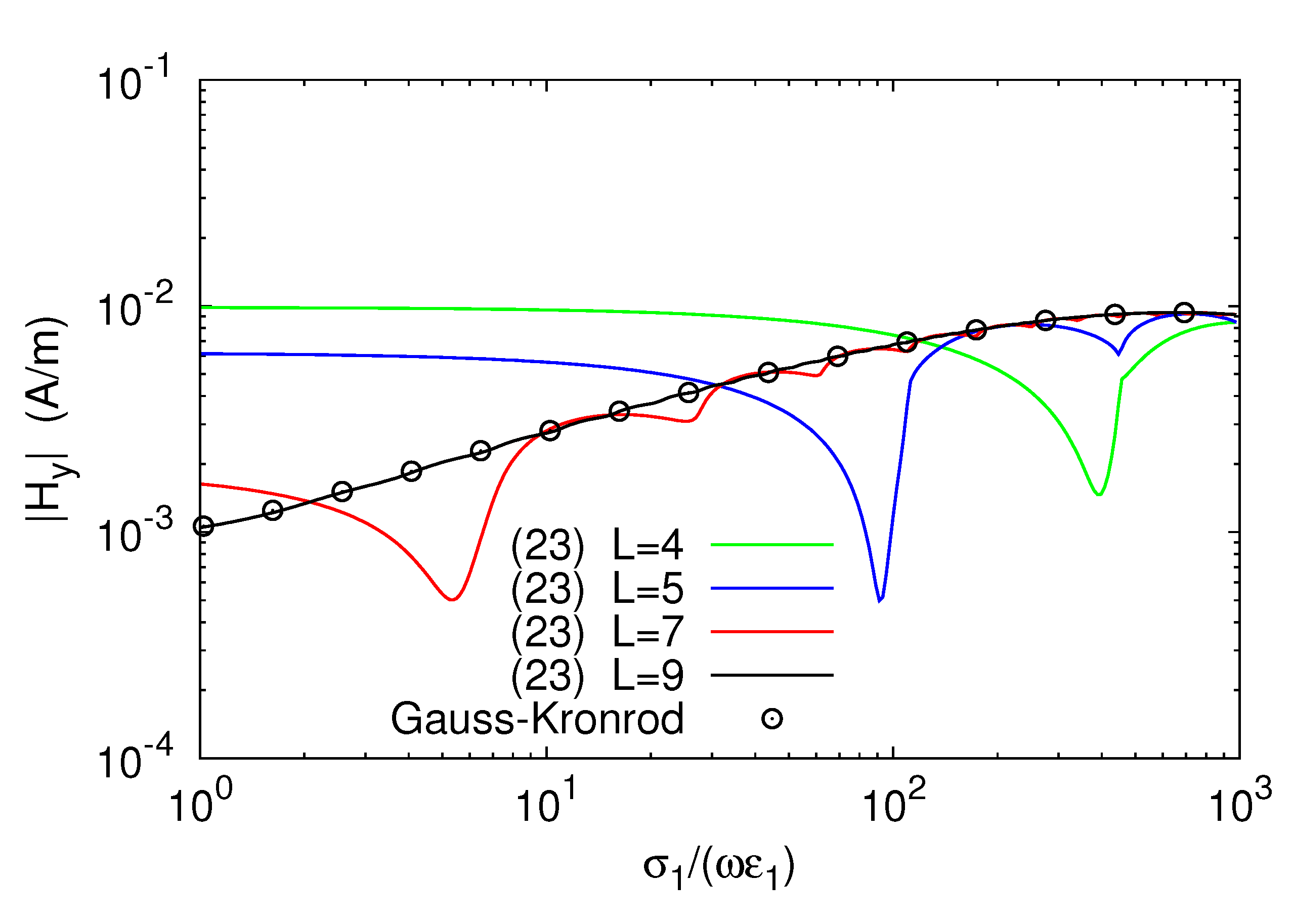
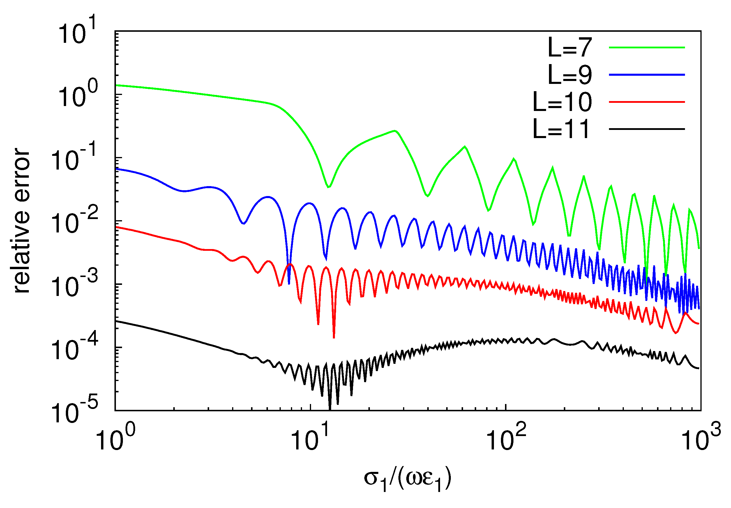
The accuracy of the result of the computation also depended on the values of the electromagnetic parameters of the lossy ground and, for instance, better accuracy was observed for larger values of the electrical conductivity . This aspect is illustrated by Figure 5 and Figure 6, which show, respectively, profiles of versus the ratio , and the relative error resulting from using (23) instead of G7-K15 scheme. Here, it is assumed that the source carried 1 A and operated at 100 kHz, and that = 20 , h = 5 m, y = 10 m, and z = 1 m. As is seen, the sequence of profiles of generated by the partial sums in (23) converged to the curve provided by the G7-K15 scheme, and perfect agreement between the analytical and numerical data was again obtained for L = 9. Furthermore, convergence was faster in the good-conductor limit (), where it sufficed to use a sum constituted by seven terms to produce sufficiently accurate results. This does not necessarily imply that the relative error generated by each partial sum in (23) always decreased as the conductivity grew. In fact, as pointed out by Figure 6, the error fluctuated around a decreasing mean value rather than being monotonically decreasing.
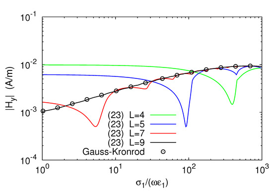
Figure 5.
Amplitude of against the normalized conductivity of the ground .
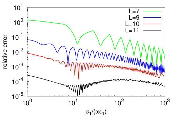
Figure 6.
Relative error of (23) as compared to G7-K15 scheme, plotted against .
The proposed method made it possible to achieve time savings compared to G7-K15 numerical scheme, while maintaining the same accuracy as the latter. In fact, on a single-core 2.2 GHz processor, the average CPU time taken by (23) to generate the profile of associated with L = 9 in Figure 5 was equal to 157 ms, while about 9 s were taken by numerical integration of (27) to produce the same outcome. This means that, limited to the considered example, the proposed approach was about 57 times faster than Gaussian integration, and, as a consequence, the numerical complexity of the former was significantly smaller than that exhibited by the latter. For the sake of completeness, the time costs of (23) corresponding to the remaining values of L depicted in Figure 5 are indicated in Table 1.

Table 1.
CPU time comparisons for the calculation of .
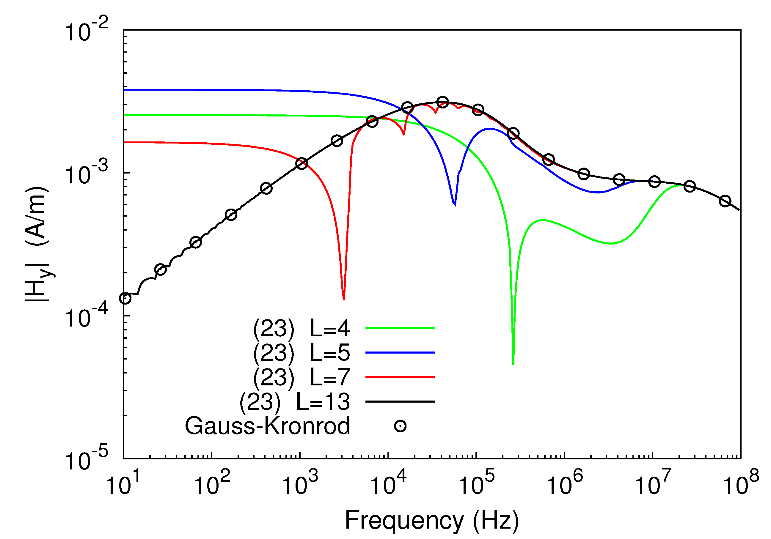
Finally, one would ask whether the proposed solution may still be used when both h and z approach zero, since it has been obtained starting from expression (9), whose integrals on the right-hand side, strictly speaking, converged only for = . This point is clarified by Figure 7, which shows the amplitude–frequency spectrum of the -field that a unit-current line source generated at a point placed 30 m apart from it, assuming that both the source and the observation point lay on a homogeneous ground with = 20 mS/m and = 10 . As is evident from the analysis of the plotted curves, the trends arising from the sequence of partial sums in (23) still converged to the curve resulting from numerical integration of (27), even if the number of terms of (23) required to approach the numerical data grew as frequency decreased.
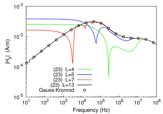
Figure 7.
Amplitude-frequency spectrum of , resulting from using both (23) and the G7-K15 scheme.
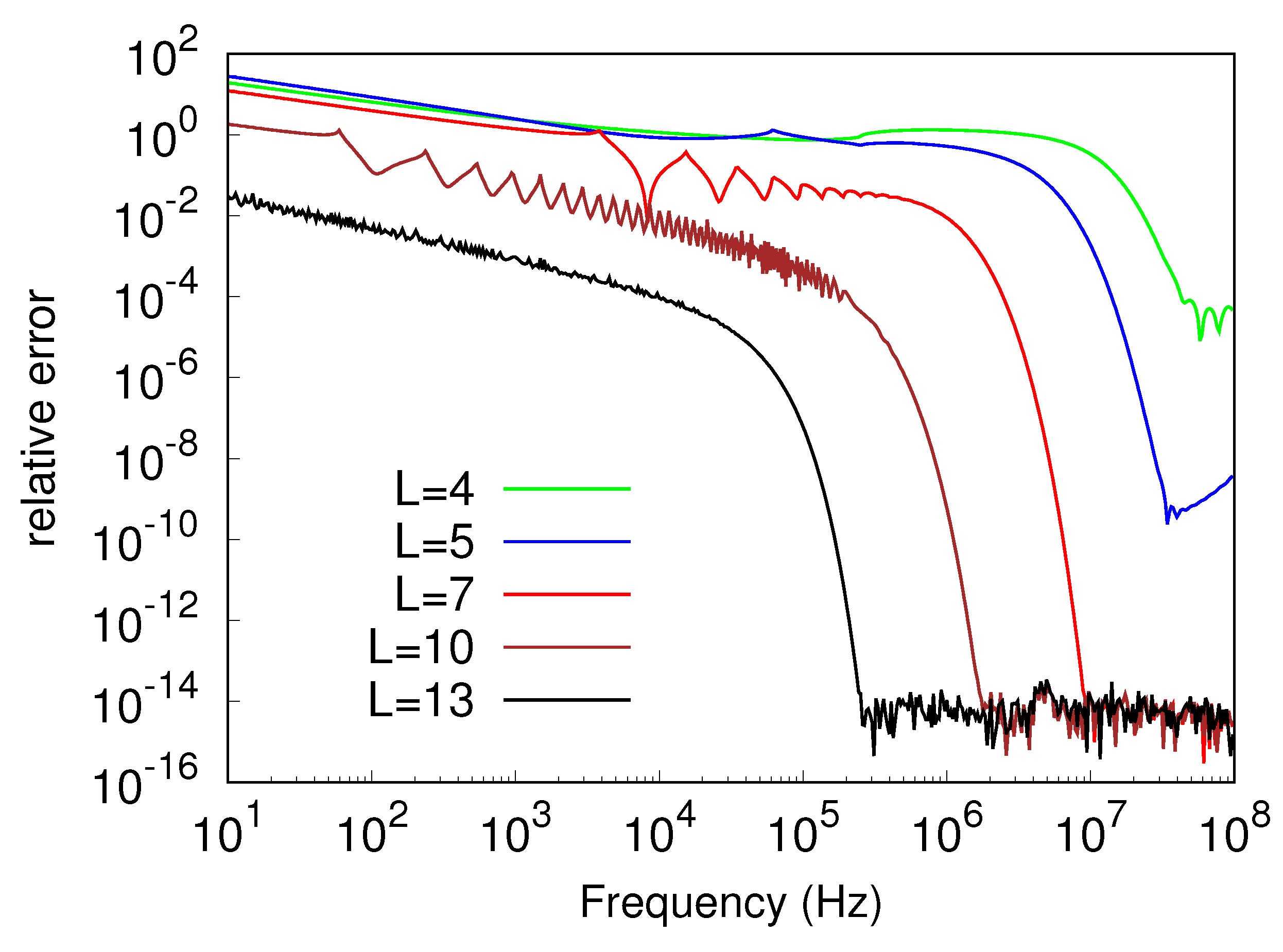
Hence, the rate of convergence of (23) depended on frequency, and convergence was faster at higher frequencies. This aspect is further investigated in Figure 8, which depicts the relative error of the outcomes of (23) plotted in Figure 7, as compared to the data arising from the G7-K15 rule. The curves of Figure 8 point out that, for a fixed L, the accuracy of the result of the computation significantly worsened when entering the low-frequency range. At the same time, they confirmed that the accuracy could always be enhanced by increasing L. This implies that, all over the considered frequency range, it holds [29]
where the symbol denotes the sequence of partial sums that originates from (23), as a result of truncating the infinite sum in (18), and where p and q are the order of convergence (OC) of the sequence and the asymptotic error constant (AEC), respectively. It is easily understood that the parameters p and q depend on the operating frequency, and that the knowledge of their values permits to acquire further information on the rate of convergence. As an example, Table 2 illustrates Lth order estimates of the OC and the AEC for the sequence corresponding to 1 kHz in Figure 7. The estimates were calculated using the well-known expressions [29]
whose limits as approach p and q [29]. As pointed out by Table 2, with increasing L, and this means that the sequence converges linearly. Moreover, convergence is accelerated by the small values of the ’s, which further reduce the remainder at any additional iteration of the sequence.
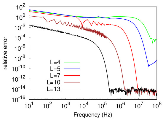
Figure 8.
Relative error of (23) as compared to G7-K15 scheme, plotted against frequency.
Table 2.
Estimated OC and AEC for the sequence .
4. Conclusions
This paper has presented a rigorous analytical approach for evaluating the time-harmonic EM field components generated in the air space by an infinite current line source located above a homogeneous lossy ground. The approach consists of expanding the non-analytic part of the integrand of the correction term in the integral expression for the axial electric field into a power series of the z-directed propagation coefficient in air. This leads to express the axial electric field as a sum of derivatives of the Sommerfeld Integral describing the direct field, which may be analytically evaluated. As a result, the electric field is given as a sum of cylindrical Hankel functions, with coefficients depending on the position of the field point relative to the line source and its ideal image. Then, explicit expressions for the magnetic field components are also derived by applying Faraday’s law. The obtained solution is not subject to simplifying assumptions, and hence is valid even when the high-frequency effects due to the displacement currents in both the air and the soil are no longer negligible. Numerical simulations have been carried out to show that the proposed approach exhibits good accuracy, while taking significantly less computation time than conventional numerical quadrature schemes used to evaluate Sommerfeld-type integrals.
Funding
This research received no external funding.
Conflicts of Interest
The author declares no conflict of interest.
References
- Alanen, E.; Lindell, I. Image calculation of electromagnetic field from power lines above a dissipative ground. Arch. Elektrotech. 1985, 68, 259–265. [Google Scholar] [CrossRef]
- Rachidi, F.; Tkachenko, S. Electromagnetic Field Interaction with Transmission Lines: From Classical Theory to HF Radiation Effects; WIT Press: Southampton, UK, 2008; Volume 5. [Google Scholar]
- Spiegel, R.J. Numerical determination of induced currents in humans and baboons exposed to 60-Hz electric fields. IEEE Trans. Electromagn. Compat. 1981, EMC-23, 382–390. [Google Scholar] [CrossRef]
- Wait, J.R. Theory of wave propagation along a thin wire parallel to an interface. Radio Sci. 1972, 7, 675–679. [Google Scholar] [CrossRef]
- Wait, J.R.; Spies, K.P. On the image representation of the quasi-static fields of a line current source above the ground. Can. J. Phys. 1969, 47, 2731–2733. [Google Scholar] [CrossRef]
- Olsen, R.G.; Young, J.L.; Chang, D.C. Electromagnetic wave propagation on a thin wire above earth. IEEE Trans. Antennas Propag. 2000, 48, 1413–1419. [Google Scholar] [CrossRef]
- Rachidi, F. A review of field-to-transmission line coupling models with special emphasis to lightning-induced voltages on overhead lines. IEEE Trans. Electromagn. Compat. 2012, 54, 898–911. [Google Scholar] [CrossRef]
- Ametani, A.; Miyamoto, Y.; Baba, Y.; Nagaoka, N. Wave propagation on an overhead multiconductor in a high-frequency region. IEEE Trans. Electromagn. Compat. 2014, 56, 1638–1648. [Google Scholar] [CrossRef]
- Micu, D.D.; Czumbil, L.; Christoforidis, G.C.; Papadopoulos, T. Semi-infinite integral implementation in the development steps of Interfstud electromagnetic interference software. In Proceedings of the IEEE 2012 47th International Universities Power Engineering Conference (UPEC), London, UK, 4–7 September 2012; pp. 1–6. [Google Scholar]
- Papakanellos, P.J.; Kaklamani, D.I.; Capsalis, C.N. Analysis of an infinite current source above a semi-infinite lossy ground using fictitious current auxiliary sources in conjunction with complex image theory techniques. IEEE Trans. Antennas Propag. 2001, 49, 1491–1503. [Google Scholar] [CrossRef]
- Wise, W.H. Propagation of HF currents in ground return circuits. Proc. Inst. Elect. Eng. 1934, 22, 522–527. [Google Scholar]
- Kikuchi, H. Wave propagation along an infinite wire above ground at high frequencies. Proc. Electrotech. J. 1956, 2, 73–78. [Google Scholar]
- Dorin, C.; Marilena, U.; Codruta, R. Electromagnetic coupling phenomena of overhead power lines in low and high frequency. In Proceedings of the 2003 IEEE International Symposium on Electromagnetic Compatibility, EMC’03, Istanbul, Turkey, 11–16 May 2003; Volume 2, pp. 1178–1181. [Google Scholar]
- Degauque, P.; Laly, P.; Degardin, V.; Lienard, M. Power line communication and compromising radiated emission. In Proceedings of the IEEE SoftCOM 2010, 18th International Conference on Software, Telecommunications and Computer Networks, Split, Croatia, 23–25 September 2010; pp. 88–91. [Google Scholar]
- Pagani, P.; Ney, M.; Zeddam, A. Application of Time Reversal to Power Line Communications for the Mitigation of Electromagnetic Radiation. In Electromagnetic Time Reversal: Application to EMC and Power Systems; Rachidi, F., Rubinstein, M., Paolone, M., Eds.; Wiley Online Library: New York, NY, USA, 2017; Chapter 5; pp. 169–187. [Google Scholar]
- Sunde, E.D. Earth Conduction Effects in Transmission Systems; Dover: New York, NY, USA, 1968. [Google Scholar]
- Pistol’kors, A. On the theory of a wire parallel to the plane interface between two media. Radiotek 1953, 8, 8–18. [Google Scholar]
- Kuester, E.F.; Chang, D.C.; Olsen, R.G. Modal theory of long horizontal wire structures above the earth—Part I: Excitation. Radio Sci. 1978, 13, 605–613. [Google Scholar] [CrossRef]
- Judkins, R.; Nordell, D. Discussion of Electromagnetic Effects of Overhead Transmission Lines Practical Problems, Safeguards and Methods of Calculation. IEEE Trans. Power Apparatus Syst. 1974, PAS-93, 892–902. [Google Scholar]
- Kostenko, M. Mutual impedance of earth-return overhead lines taking into account the skin-effect. Elektritchestvo 1955, 10, 29–34. [Google Scholar]
- Chang, D.C.; Olsen, R.G. Excitation of an infinite antenna above a dissipative earth. Radio Sci. 1975, 10, 823–831. [Google Scholar] [CrossRef]
- Olsen, R.G.; Kuester, E.F.; Chang, D.C. Modal theory of long horizontal wire structures above the earth—Part II: Properties of discrete modes. Radio Sci. 1978, 13, 615–623. [Google Scholar] [CrossRef]
- Déri, Á.; Tevan, G. Mathematical verification of Dubanton’s simplified calculation of overhead transmission line parameters and its physical interpretation. Arch. Elektrotech. 1981, 63, 191–198. [Google Scholar] [CrossRef]
- Tevan, G.; Deri, A. Some remarks about the accurate evaluation of the Carson integral for mutual impedances of lines with earth return. Arch. Elektrotech. 1984, 67, 83–90. [Google Scholar] [CrossRef]
- Mohsen, A.; Shafai, L. On the image representation of the fields of a line current source above finitely conducting earth. Can. J. Phys. 1981, 59, 117–121. [Google Scholar] [CrossRef]
- Abramowitz, M.; Stegun, I.A. Handbook of Mathematical Functions: With Formulas, Graphs, and Mathematical Tables; Courier Corporation: Massachusetts, MA, USA, 1964; Volume 55. [Google Scholar]
- Palacky, G.J. Resistivity characteristics of geologic targets. In Electromagnetic Methods in Applied Geophysics; Nabighian, M.N., Ed.; Society of Exploration Geophysicists: Tulsa, OK, USA, 1988; Chapter 3; Volume 1, pp. 52–129. [Google Scholar] [CrossRef]
- Ward, S.H.; Hohmann, G.W. Electromagnetic theory for geophysical applications. In Electromagnetic Methods in Applied Geophysics; Nabighian, M.N., Ed.; Society of Exploration Geophysicists: Tulsa, OK, USA, 1988; Chapter 4; Volume 1, pp. 130–311. [Google Scholar] [CrossRef]
- Householder, A.S. The Numerical Treatment of a Single Nonlinear Equation; McGraw-Hill: New York, NY, USA, 1970. [Google Scholar]

Publisher’s Note: MDPI stays neutral with regard to jurisdictional claims in published maps and institutional affiliations. |
© 2020 by the author. Licensee MDPI, Basel, Switzerland. This article is an open access article distributed under the terms and conditions of the Creative Commons Attribution (CC BY) license (http://creativecommons.org/licenses/by/4.0/).