Abstract
We propose a new end-to-end scene recognition framework, called a Recurrent Memorized Attention Network (RMAN) model, which performs object-based scene classification by recurrently locating and memorizing objects in the image. Based on the proposed framework, we introduce a multi-task mechanism that contiguously attends on the different essential objects in a scene image and recurrently performs memory fusion of the features of object focused by an attention model to improve the scene recognition accuracy. The experimental results show that the RMAN model has achieved better classification performance on the constructed dataset and two public scene datasets, surpassing state-of-the-art image scene recognition approaches.
1. Introduction
Scene recognition is one of the important directions in image classification, as scene recognition technology can be applied to a broad range of applications, such as image and video retrieval, target recognition and detection, robotics applications, image enhancement, etc. Since the Massachusetts Institute of Technology (MIT) held the first Scene Understanding Symposium in 2006, scene image recognition has attracted widespread attention from the researchers all over the world. Generally speaking, scene images often contain multiple target objects that are combined in space to form a scene. For example, a scene of tennis game consists of caddie, tennis player, racket, referee, etc., while tall buildings, streets, people flow, and vehicles constitute a scene of an urban area. The purpose of scene image recognition is to quickly and efficiently divide pictures into categories to which their semantics belong, so as to satisfy the requirement of classifying pictures and managing pictures. Compared with traditional image classification, the number of dataset categories in the scene recognition task is large, but the training dataset is relatively small. At the same time, due to the differences in the content of the scene itself, there are often large intra-class differences and high inter-class visual similarities for scene recognition, especially in the indoor scene classification task.
In recent years, with the rapid development of artificial intelligence and deep learning technology, more and more research institutions and enterprises began to focus on the scene recognition. They not only announced scene datasets such as Places [1], Sun 397 [2], MIT Indoor 67 [3] but also proposed effective algorithms to improve scene recognition accuracy. With the efforts of researchers, the accuracy of scene recognition is constantly improved, especially with the boom of deep learning algorithms. Although scholars have proposed many scene recognition approaches, each method is mainly aimed at a specific dataset, and its recognition performance is often unsatisfactory. With the development of deep learning algorithm, scene recognition technology has achieved great success, but the various challenges mentioned above have not been completely solved in the academic and industrial domain. Therefore, the research of scene image recognition is still a challenging topic in the field of computer vision technology.
In this paper, we propose a scene image recognition model named the Recurrent Memorized Attention Network (RMAN) model, which classifies a scene image based on the recurrently locating and memorizing objects with attention mechanism. To be specific, the RMAN model pays attention to different objects in an image through the attention localization module and employs the LSTM (Long Short-Term Memory) network to memorize the features of an object focused by the attention model and classify accordingly. This algorithm realizes end-to-end scene recognition and performs well on two public datasets and a constructed dataset. The main contributions of our work can be summarized as follows:
- (1)
- We propose a novel framework for an end-to-end scene recognition task that performs object-based scene classification by recurrently locating and memorizing objects with an attention mechanism.
- (2)
- Base on the proposed framework, we propose a multi-task mechanism that contiguously attends on the different essential objects in a scene image and recurrently performs memory fusion of the features of object focused by an attention model to improve the scene recognition accuracy.
- (3)
- We construct a new scene dataset named Scene 30, which contains 4608 color images of 30 different scene categories, including both indoor and outdoor scenes.
The rest of paper is organized as follows. Section 2 introduces the related work about scene recognition, and our proposed RMAN model for scene recognition will be illustrated in detail in Section 3. Experimental results will be presented and discussed in Section 4. Section 5 concludes the paper and discusses the future work.
2. Related Work
In general, there are two types of scene recognition techniques in the literature based on the way in which scenes are classified. The first one is a feature-based approach that classifies images based on low-level features extracted from the scene images. The second one is an object-based approach, which combines objects detected in an image to determine the category of the scene images.
2.1. Low-Level Image Feature Based Scene Recognition
The low-level feature-based scene recognition method generally extracts discriminative features from scene images as the scene representation, followed by a semantic model constructed based on this scene representation. Scene feature representation not only extracts general information from similar scene pictures but also excavates distinguishing features in different types of scenes. The current scene feature representation methods are mainly divided into two categories: manually crafted feature representation methods and deep learning-based feature representation methods. Typical manually crafted feature representations include GIST [4], OTC [5], CENTRIST [6], and mCENTRIST [7]. GIST transforms the global scene image into a high-dimensional feature vector, but it failed to explore the local structure information of the scene image, especially for indoor scenes recognition, where indoor scenes often have complex spatial distributions. Unlike global features, local features such as OTC, CENTRIST, and mCENTRIST first describe each local block and then fuse all local features together. These methods explore the structural characteristics and texture information of scene images. However, this information is far from satisfying the requirements of complex scenarios. Recently, a deep learning-based representation method represented by a Convolutional Neural Network (CNN) [8] has explored high-level semantic information of images and has achieved significant progress in scene classification accuracy. These deep models learn discriminative visual features directly from the original dataset in an end-to-end manner. Thanks to the large-scale datasets, such as Places [1], ImageNet [9], etc., and the development of computing resources, some successful and effective depth models have been continuously proposed and widely used in the field of image analysis and understanding, which include AlexNet [10], VGGNet [11], GoogLeNet [12], ResNet [13], DenseNet [14], etc. Compared with the traditional manually crafted feature representation methods, convolutional neural networks have stronger modeling and learning capabilities, and they can learn more abstract and robust visual representations.
Once the features have been extracted, the classifiers can be constructed to perform a scene recognition task. In general, scene classification methods can be divided into two categories: generative models and discriminative models. Generative models usually model the joint probabilities of training samples and employ hierarchical Bayesian methods to describe various relationships in a scene. Typical generative model classifiers include Conditional Random Field (CRF) [15], Hidden Markov Model (HMM) [16], Markov Random Field (MRF) [17], Latent Dirichlet Allocation (LDA) Model [18], and multi-binary classifier referred to as error correcting output code (ECOC) [19]. Although the generative model can deal with a small training dataset problem well, these methods all need to construct complex probability graph models, which will lead to the complicated learning process and the high computational cost. The discriminative model extracts dense descriptors in the image and then encodes them into a fixed-length vector to learn a reasonable classifier. The representative discriminant model methods include boosting, logistic regression, Support Vector Machine (SVM), and so on. Among them, SVM is widely used in scene recognition tasks [20]. In [21], the authors classify scenes images with AlexNet CNN followed with a transfer learning module to optimize the output and get a speedy progress in the applied model. Unlike generative models, a discriminant model makes it easier to learn classifier parameters.
2.2. Object-Based Scene Recognition
Combining objects detected in the image for scene recognition is a straightforward and intuitive approach, and it can assist in distinguishing very complex scenes that might otherwise prove difficult to do using standard feature-based approaches. Li [22] and Antonio [23] explored the relationship between the overall scene image and local objects, while Myung [24] and Li [25] studied the correlation of the object collection appearing in the same scene category. Wu [26] focused their attention on objects in a scene and proposed the concept of a “meta object”. An image is represented by a collection of “meta objects”, and superior performance on high-level visual recognition tasks can be achieved with simple regularized logistic regression. Cheng [27] proposed a scene-oriented Semantic Description of Object (SDO) approach in order to increase the inter-class distance and reduce the intra-class differences in scene recognition tasks. In our previous work [28], we proposed exploiting the relations between the entire image and the manually configured objects in an image with the ancillary information from the scene graph to recognize an image scene. In [29], the deep visually sensitive features obtained by feeding the pre-trained CNNs with the scene images enhanced by detected saliency are proved to be effective for scene recognition. It can be seen from these methods that in order to extract better scene features, more and more researchers focus on scene objects, and most of the models contain similar object positioning modules. However, most of these methods require high computational cost to generate candidate frames, and the overall framework is mostly not in an end-to-end manner.
In recent years, an attention model [30,31,32] has been greatly successful in the field of Natural Language Processing (NLP). The success of the attention model in the field of NLP has also promoted its development in some computer vision-related tasks, especially in the direction of fine-grained image classification. Research methods [33,34,35] have gradually evolved from the previous supervised methods to the current weakly supervised method that only employs the category label information of the image to perform fine-grained classification on the image. The attention model automatically pays attention to information of different objects in fine-grained images, such as a bird’s beak and wings, and then extracts features for classification. Inspired by this, we propose a Recurrent Memorized Attention Network (RMAN) model for scene recognition, which simulates the cognitive process in human cognition in which our eyes scan the objects in the scene, while our brain recurrently memorizes them and makes judgment.
3. Scene Recognition Based on RMAN
In this section, we propose an automatic scene recognition approach based on the RMAN model elaborately. Figure 1 demonstrates the framework of the proposed approach, which consists of three modules: feature extraction, attention localization, and recurrent memorized attention. The feature extraction module tries to extract the global representation of a scene image, which will be the preliminary step for the subsequent modules. Then, the attention localization module and recurrent memorized attention module are alternatively performed to recurrently shift the focus on the different objects in an image and integrate these objects together to characterize the scene category, which simulates the cognitive process in human cognition that keeps our eyes scanning objects in an image and merges them together in our mind until we can judge the scene category for this image. The attention localization module aims to localize the attention area of a scene image based on its global representation by constraining the loss function. The purpose of the recurrent memorized attention module is to perform memory fusion of the features of an object focused by the attention model to improve the scene recognition accuracy. The attention localization module and recurrent memorized attention module will alternate iteratively during the scene recognition process, and in each iteration, the recurrent memorized attention module will regress the parameters required for the attention localization module in the next iteration. The RMAN model will iteratively perform the above process several times to discover the attention area and memorize features of the discovered attention area for classification.
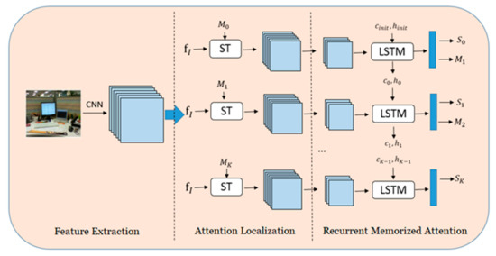
Figure 1.
Proposed framework of recurrent memorized attention network.
In what follows, we will detail each step of the proposed framework.
3.1. Feature Extraction Module
The feature extraction module is employed to extract the features from scene images, which is illustrated in Figure 2. Due to the excellent feature extraction ability for images and relatively simple structure of the VGGNet [11], we adopt the VGG-16 model pre-trained in ImageNet to obtain the global representation of the scene image and the feature of the scene image. The structure of the feature extraction module can be shown as in Figure 2. The input image size of the proposed feature extraction network is expanded to a 512 × 512 × 3, while in a typical VGG-16, it is 224 × 224 × 3, for the purpose of providing enough space for attention localization module. We employ a 3 × 3 convolution kernel with a stride step of 1 and a padding parameter with 1, and a 2 × 2 max pooling strategy. As Figure 2 shows, the original image input to the feature extraction module is 512 × 512 × 3 RGB image, which can be denoted as Ii. After two convolution operations of 64 convolution kernels, one pooling is performed, and then after two convolutions of 128 convolution kernels, one pooling is performed, which is followed by three 256 convolution kernels. After the convolution, a pooling operation is performed. Finally, a convolution operation of three 512 convolution kernels is repeated twice. We use the feature extracted from the last convolutional layer as the initial feature of the attention-positioning module, which can be denoted as fI.
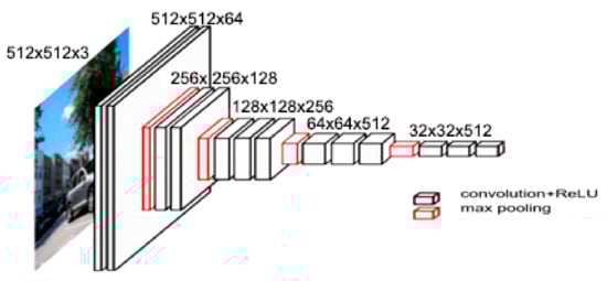
Figure 2.
The structure of the feature extraction module.
The function of the feature extraction module can be described by the following:
where Wa represents all the parameters used in the feature extraction module, and the operator * represents the convolution, pooling, and activating operation involved in the feature extraction module.
Based on the global feature fI of the scene image obtained by the feature extraction module, the deep semantic information of the scene image is captured. Similar to the idea of the Faster-RCNN model [36], we will locate the attention area based on this global feature representation, instead of extracting the attention area of the original image and sending it to the deep convolutional neural network. The advantage of the replacement of a raw image with the global feature representation for attention location is obvious, as it reduces the parameters of the network, accelerates the convergence of the network, and facilitates optimal scene classification.
3.2. Attention Localization Module
In the past few years, the framework of a visual attention-based scene recognition model has mainly depended on the local semantics expressed by the objects in the image, which can be extracted from a large number of candidate regions in the image. As a result, it requires large computational resource and increases the time for training and testing. In our proposed model, we try to embed an attention localization module in the RMAN model to locate the essential objects of the scene.
Inspired by the research work from Google Deep Mind, we employ the Spatial Transformer Networks (STN) [37] as our structure of the attention localization module. Convolutional neural network defines an extremely powerful model for scene classification, but it is still limited by the spatial invariance property of the input data in a computationally efficient manner; therefore, a new spatially deformed network structure so-called the Spatial Transformer Network (STN) is employed in our proposed framework. The Spatial Transformer (ST) is the core component of the STN, which can be embedded in the traditional convolutional neural networks as a plug-in module. It can provide the traditional convolutional convolution network with the functionality such as rotation, translation, scaling, and so on in the feature extraction stage, and we hope that with the aid of ST, the convolutional neural network can learn how to deform the deep features by itself. As a result, our proposed scene classification approach achieves good performance, as it is invariant to translation, scaling, rotation, and generic warping of objects in the image.
The specific structural diagram of the Spatial Transformer can be found in [37], which is mainly composed of three parts: Localization Net, Grid Generator, and Sampler. Assume U and V represent the deep features of the network before and after the ST transformation, respectively, and θ is the transformation parameters returned by the local network. The local network is mainly used to return the spatial transformation parameters. Its input is the features before transformation, and then, it passes through a series of hidden network layers, such as the convolutional layer, pooling layer, fully connected layer, regression layer, etc., and the output is the spatial transformation parameter. The dimension of θ depends on the specific transformation type selected by the network. If an affine transformation is selected, it is a 6-dimensional (2 × 3) vector. If a projection transformation is selected, it is a 9-dimensional (3 × 3) vector. In our model, θ is a 6-dimensional vector of 2 × 3, and it can be defined as:
where θ11 and θ22 are mainly used to control the scaling changes of the feature size, θ13 and θ23 are used to control the translation changes, and θ12 and θ21 are mainly used to control the rotation changes.
Since the essential object in the scene image basically does not need to be rotated in our dataset, the transformation matrix M in the experiment is defined as follows:
The grid generator mainly builds a sampling grid based on the transformation matrix M returned by the local network, which are the outputs obtained by sampling transformation of a set of input features. Assume that the pixel coordinates in the feature image U are (xs,ys) and the corresponding pixel coordinates in the transformed feature image V are (xt,yt), which is a spatial transformation function. The correspondence between (xs,ys) and (xt,yt) can be written as:
As illustrated in [37], the sampler uses the sampling grid and the input feature map to generate output at the same time, and it obtains the result after the input features are transformed. The above process is also called Differential Image Sampling, which is expected to be a formally differentiable image sampling method, in order to keep the entire network trainable by back-propagation, with a relatively simple bilinear difference formula to sample the true pixel value in the corresponding position.
In our proposed framework, the ST layer is mainly used for attention localization and feature extraction for the region of the essential objects. It is assumed that during the k-th iteration, we extract the features of the target region, which can be denoted as fk, from the global feature of scene image fI. The calculation process of the entire attention positioning module is as follows:
- (1)
- Initial or regress by LSTM network (described in Section 3.4) to generate the parameter matrix M required for transformation.
- (2)
- Coordinates mapping: get the coordinate grid of the corresponding fI based on the coordinates of fk.
- (3)
- Bilinear interpolation: generate a feature map fk corresponding to the attention area through bilinear interpolation.
The k-th iteration feature map fk calculated in the above module can be formulated as shown in Equation (5):
where st(∙) represents the spatial transformation function of the Spatial Transformer, which contains a coordinates mapping step and bilinear interpolation step in the above attention positioning module, and fI represents the global features of the scene image extracted by the feature extraction module. Mk is the spatial transformation matrix estimated from the previous iteration. In the first iteration of the network, we initialize M0 as
The example of coordinate mapping can be shown in Figure 3. Figure 3a shows the coordinate grid mapping between feature maps, and Figure 3b represents the coordinate grid mapping between input images. It can be seen that the Spatial Transformer (ST) can achieve the attention area localization.
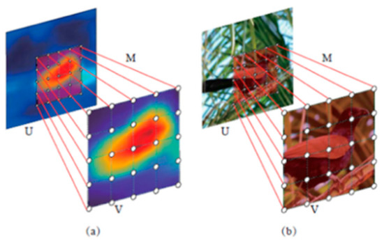
Figure 3.
Illustration of coordinate grid mapping. (a) The coordinate grid mapping between feature maps (b) The coordinate grid mapping between input images.
3.3. Recurrent Memorized Attention Module
During the training phase, the attention localization module can continuously find the attention region—that is, the box area containing essential object for a scene. How to make the network recurrently find the attention area and realize the end-to-end training is a challenge, and how to better integrate the features of the constantly generated essential object area is another challenge for us. In order to solve these problems and improve the classification accuracy of scene images, we propose a novel recurrent memorized attention model to perform memory fusion of features of object focused by the attention model. As shown in Figure 1, we employ the LSTM network structure to continuously and recurrently memorize the characteristic features of the attention area for the current stage and return the position parameters required for attention location in the next stage.
In order to prevent the curse of dimensionality of the LSTM input, for each spatial transformer in the attention location module, we follow with a convolution layer and a maximum pooling layer. The LSTM network module accepts the output of the pooling layer (denoted as ft) as the input to calculate the state of the memory unit and the hidden layer. The specific calculation is described in Equation (7):
where relu(∙) is a rectified linear function, σ represents the sigmoid activation function, tanh( ) means the hyperbolic tangent activation function, hk-1 and ck-1 represent the hidden state and memory unit of the previous iteration cycle, respectively, and ik, gk, and ok respectively denote the output of the input gate, forget gate, and output gate in the LSTM network structure. ⊙ represents point-by-point multiplication operation, and these multiplication gates can guarantee that the LSTM module remains robust and avoids the phenomenon of gradient disappearance and explosion during training.
The memory unit ck encodes the features in the previous k−1 attention areas. Our task will benefit from it in the following ways. First of all, the previous work [38,39] shows that different scene categories often show strong symbiosis in the scene graph. Therefore, it is easy to infer to which scene category the image belongs based on the currently recognized object combined with the object of the previous cycle. For example, for an image containing the object “groom”, we cannot determine whether it is a “wedding” scene category or a “wedding photo shoot” scene category, but if we add bride, groomsman, meeting room, and guest in this image, we can easily determine the scene category to which it belongs. Second, all the features of the attention area before the memory unit encoder can help us find all the relevant object areas useful for classification, while considering the feature information captured during the previous iteration and implicitly enhancing the diversity and complementarity of the attention areas. The hk in Equation (7) denotes the hidden layer state in the LSTM structure during the k-th iteration, and it will be used for the next stage of multi-task learning.
As shown in Figure 1, the final output of recurrent memorized attention module is the scene category label to which the image belongs and the spatial deformation parameter matrix Mk+1 required for the next iteration. Therefore, we need a multi-task mechanism that allows us to append a classification submodule and a position parameter regression submodule to perform classification and regression based on the hidden layer state hk of the LSTM structure. The calculation formulas are expressed as Equation (8):
where sk denotes the classification probability of the k-th attention area captured by the proposed attention localization module, and Mk+1 represents the spatial deformation parameter matrix required by the attention localization module in the next iteration. During the first iteration of network training (k = 0), the given initial spatial deformation parameter matrix is as described in Equation (6), and the matrix M in the next iteration is obtained from the LSTM structure regression in the current step. The network model will output the predicted probability of the category to which the feature belongs during each iteration. It simulates the cognitive process in human cognition, which keeps our eyes scanning objects in an image and merges them together in our mind until we can make a judgment for the scene category of this image. As a result, the accuracy of classification can be improved.
With the scene data being continuously input to the model in the training stage, the RMAN model will discover the attention area by controlling the constraints of loss for network, memorize and extract features of the discovered attention area for classification by employing the LSTM structure, and eventually reach convergence.
3.4. Process of Model Learning
In the process of training the proposed RMAN model, we need to design a suitable and effective loss function, which will constrain the network to find the attention area recurrently and to generate the optimal scene classification. In response to these two tasks, we have designed two loss functions to control the network for the recurrent discovery of attention areas and scene classification. This section will introduce the design and implementation of different loss functions in the model learning process.
As we mentioned in Section 3.3, the LSTM structure in the RMAN model outputs the classification probability of scene pictures during each iteration. In the process of model learning, we employ a multi-class Cross Entropy Loss Function to optimize the network model for classification tasks. Assume that there are totally N scene categories in the dataset, and each picture xi has its own semantic category label yi, where yi is represented as a one-hot vector; that is, each position index in the vector represents a certain scene category, and the one-hot label corresponding to picture xi is set to 1 at the position of the corresponding category, and the rest is 0. For example, in the MIT Indoor 67 public dataset, there are totally 67 categories. The scene category to which the current image belongs is church. We assume its position in the index as 3, and the corresponding label of this picture is [0,0,1, …, 0], which is a 1 × 67 vector.
Assume that during the k-th iteration of the picture xi, the classification probability predicted by the network is sk, the label of the picture is yi, and the model is set to locate three attention object regions. The classification loss function of the RMAN model is shown in Equation (9):
The above cross-entropy function characterizes the probability distribution distance between the actual output and the expected output. In the training process of RMAN model, we expect to approximate the classification output of the model as close as possible to the one-hot label of the image by minimize the loss function. In the model training phase, we employ the Stochastic Gradient Descent (SGD) method to optimize the loss function so that for each iteration, the value of the loss function is getting smaller and smaller, which will improve the classification accuracy of the scene image. The training process will be stopped when the entire loss function is converged. In the testing stage, the final classification label of the scene image xi is obtained by summing over the classification output vectors of the attention areas for each iteration and finding the index of the maximum value of the output vector.
As discussed above, the RMAN model obtains the final scene category information of the image by aggregating the classification probability of the attention area in this image. Therefore, how to accurately locate the attention area that is useful for classification has become a key problem for the RMAN model. At the stage of locating the attention area of the RMAN model, we hope that the network adaptively discovers the essential objects of the scene and thereby extracts more discriminative image features and further improves the accuracy of scene classification. We use the LSTM network structure to memorize the features of the attention area found recurrently. Of course, we can employ the loss function in the scene classification described in the previous section as the final objective function. However, the experimental results show that this strategy will bring several problems:
- (1)
- Positioning redundancy. The constraint of the loss function on the RMAN model will lead to the Spatial Transformer (ST) layer being trapped to the same area (local minimum) in the image, which results in the extracted features of essential scene object being redundant. Therefore, although the number of network iterations is increased, the essential objects area found in each iteration are actually similar or exactly same to previous one, which is contradictory to the model design as the increasement of the complexity of the network does not bring improvement to the final scene classification result.
- (2)
- Ignoring the small objects. The Spatial Transformer (ST) layer will locate relatively large objects and ignore the small objects for model classification. Actually, in the scene classification task, due to the complexity and diversity of the scene images, the small objects in the scene image often have an important role for scene recognition. For example, small objects such as “mouse” and “telephone” in an image are important to characterize the office scene category.
In order to solve above two problems, we try to enforce the Spatial Transformer module scanning the essential objects in a scene image with the following two constraints, the so-called anchor constraint and scale constraint.
- Anchor Constraint
As it is not necessary to perform rotation transformation on the image features, the simplified spatial transformation parameter matrix M is shown in Equation (3). There are four unknown variables (sx, sy, tx, ty) in an image to control the parameter of the image features; among them, variables tx and ty are used to control the image translation. When the RMAN model employs the cross-entropy loss function for optimization, the positioning redundancy problem described above will appear. In order to solve this problem, we impose constraints on the translation variables tx and ty so that the attention focuses will be continuously transferred to different parts of the image. During the initial step of the RMAN model (k = 0), we obtain the global features of the image by initializing the transformation matrix. In the subsequent iteration, the ST layer will focus on different local objects. For example, during the first iteration, the attention will first focus on the position of the center area of the image where we assume the existence of the useful objects for classification in default. Therefore, we can constrain the ST structure to scan the center area of the image. During the second iteration, we assume that the location of interest is a certain distance from the center point of the image, and in the third iteration, we assume that the location of interest is a bit far from center point of the image compared with it in the second iteration. Based on these assumptions, we can divide the entire image into three regions, as shown in Figure 4. Figure 4 illustrates that we set a center point of the image as the origin and draw a circle with a radius of 0.3 and a circle with radius of 0.6, which divides the image into three regions: the center area within a circle of radius of 0.3, the annulus area between a circle of a radius of 0.6 and a circle of a radius of 0.3, and the remaining area outside the circle of a radius of 0.6.
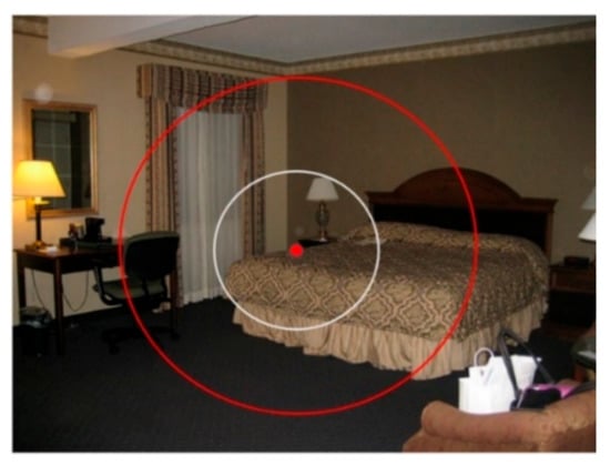
Figure 4.
Illustration of anchor constraint.
At the beginning of the learning process for the RMAN model, the spatial transformation matrix M0 is initialized according to Equation (6). The initial values of tx and ty are set to 0, which means the attention focus is located in the center area of the image. Then, in the first iteration, we constrain the translation parameters (tx, ty) to be within a circle with a radius of 0.3, and in the second iteration, we constrain the translation parameters to locate the attention focus within an annulus formed between a circle with a radius of 0.6 and a circle with a radius of 0.3. The final constraint locates the attention focus outside the circle with a radius of 0.6, where tx, ty∈[−1, 1]. Anchor constraints can be expressed as follows in Equation (10):
where
- Scale Constraint
The scale constraint is mainly designed to solve the problem in which the attention positioning module prefers large objects and ignores the small objects. Therefore, we put constraints on the scale parameters sx, sy to solve this problem.
We propose a loss function to constrain sx and sy to a range of intervals. The loss function is described by Equation (14):
where
However, the definition of above constraints cannot avoid variable sx, sy to be negative, which means that the objects in the attention area will be flipped horizontally or vertically. In order to solve the problem of spatial flipping of the positioning objects, we propose a positive constraint of scale parameters accordingly. The positive constraint attempts to control the scale parameters sx and sy to always be positive, which is shown in Equation (16):
By applying the above two constraints on the spatial transformation matrix M in the attention positioning stage, the final positioning loss function is the sum of the anchor point constraint and the scale constraint. The final positioning loss is described by Equation (17):
where and represent the weights of different loss functions. In the experiments, we set them to 0.01 and 0.1, respectively.
As a multi-tasking framework, the RMAN model classifies a scene image according to the characteristics of memorized objects. Therefore, the overall loss function of the RMAN model should include classification loss and positioning loss, which is expressed as shown in Equation (18):
Among them, in order to balance the classification and positioning loss, we set up φ = 0.1 so that scene classification is still the main task of RMAN, while considering the object positioning that assists image classification. The entire model is optimized using the Stochastic Gradient Descent (SGD) optimizer algorithm. When the whole loss function approaches a stable minimum, the training process is terminated to converge.
4. Experimental Result
In this section, we will evaluate the performance of the RMAN model on two public datasets and a constructed dataset. Before the performance evaluation, the experiment setting, the model configuration, and evaluation measures for the proposed model in scene recognition will be presented.
4.1. Dataset
The performance of the proposed method for automatic scene recognition is evaluated by the experiments on the three datasets: our constructed dataset, the so-called dataset scene 30, the MIT Indoor 67 dataset, and the SUN-397 dataset.
Scene 30: To construct Scene 30, we employ Visual Genome [40] as our source dataset, as it contains a lot of indoor and outdoor scene images with scene graphs. The constructed Scene 30 contains 4608 color images of 30 different scenes including both indoor and outdoor scenes. The number of images varies across categories with at least 50 images per category. As the images from Visual Genome are not categorized into any scene class, we manually categorize them into 30 scene classes that we predefined. The list of these 30 scene classes and the number of images included is shown in Figure 5. We split 85% of each class from the entire dataset for training and the rest as a test set. Figure 6 shows several indoor and outdoor examples from the Scene 30 dataset.
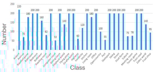
Figure 5.
Scene classes and the number of images included in Scene 30 dataset.
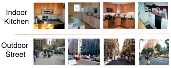
Figure 6.
Several indoor and outdoor examples from the Scene 30 dataset.
MIT Indoor 67: Unlike the Scene 30 dataset, the MIT Indoor 67 dataset contains only indoor scene images, and the scene dataset mainly covers five major categories, namely “shopping mall”, “family”, “public place”, “leisure place” and “office area”, which can be further subdivided into 67 Small scene categories, such as “Bedroom”, “Bakery”, “Church”, “Bar”, and so on. The dataset has a total of 15,620 scene pictures, and each scene category has a different number of images, but each category contains at least 100 images, and all are in JPG format. Compared with the outdoor scenes, the intra-class similarity for indoor scenes is high, so classification for indoor scenes is more difficult. MIT Indoor 67 has become the most commonly used public dataset for indoor scenes in the field of scene recognition. According to the experimental configuration protocol described by Antonio Torralba [3], which samples n positive examples and 3n negative examples for training one versus another classifier for the d category, we use 80 images in each class as the training set and the remaining images as the test set, ensuring that there are more than 20 testing samples in each class.
SUN-397: A large-scale scene dataset includes 397 distinct scene categories and 108,754 color images with at least 100 images per category, and the categories comprise different kinds of indoor and outdoor scenes with tremendous objects and alignment variance, which brings more complexity for scene recognition. According to the experimental configuration protocol described [2], we select 100 images from each category and use 50 images in each class as the training set and the remaining images as the test set.
4.2. Experimental Configuration
The machine used in the experiments in our experiments is Intel-2620 V4 CPU 2.1GHz × 8 cores, GeForce GTX TITAN X, RAM 128G, with Ubuntu 16.04 operating system, and Pytorch 0.4.1 deep learning framework.
For the three datasets in our experiment, the RAMN model employs the convolution neural network VGG-16 as the basic framework to extract the global features of the image. In the training phase, we employed a two-stage strategy to initialize the parameters of the RAMN Model. First, the VGG-16 network in the feature extraction module was pre-trained on the ImageNet, and after the fine tuning, the network was able to capture features in the scene dataset for the classification tasks. Secondly, the layer parameters of neural network in the attention localization module and recurrent memorized attention module are initialized by the Xavier algorithm [41]. After initialization, all the scene images are first uniformly deformed to the size of N × N and then randomly cropped to (N−64) × (N−64) size. Among them, the random horizontal flip strategy is also used in the training examples for data enhancement. In the experimental setup, we set N = 512; that is, the image deformation size is 512, and the random crop size is 448 × 448. We employ the Stochastic Gradient Descent (SGD) optimizer in our optimization process, with a batch size of 16 and a momentum of 0.9. The initial learning rate is set to 0.00001, and then every 30 epochs, the learning rate changes by 0.1 times as before. The network model is trained for 50 epochs, and the network model with the lowest loss on the validation set is finally retained for testing.
In the test phase, the RMAN model first deformed the scene image to a size of 512 × 512, and then cropped five areas on the deformed image and sent them to the model for testing. The five blocks are 448 × 448 in size and are positioned at the corners and center of the original image. By averaging the classification probability output during each iteration of the RAMN model, the final classification representation of the scene image can be obtained.
4.3. Results and Discussion
The classification accuracy is selected as the evaluation measurement of the proposed model. The calculation formula is shown in Equation (19).
where positive denotes the number of images that the classifier predicts is correct, and negative is the number of images that the classifier predicts is wrong.
On the Scene 30 dataset, we evaluate the classification performance of the proposed RMAN model and some state-of-the-art approaches. Table 1 shows the classification accuracy of different methods on the Scene 30 dataset. As we mentioned before, the basic framework of the feature extraction module in the RMAN model is VGG-16. Therefore, in the experiment, we introduce the model obtained by fine-tuning the pre-trained VGG-16 network as the baseline. The experimental results show that the accuracy of scene classification is improved by 6.81% with the attention localization of essential objects and recurrently memorizing the attentional objects by the RMAN model. At the same time, the performance of the RMAN mode is better than that of PlaceNet and HybridNet. In addition, the classification accuracy of the RMAN model even is better than the Constructed Knowledge Sub-Graph Learning approach [28] with the improvement of 1.03%, while the Constructed Knowledge Sub-Graph Learning approach needs the knowledge sub-graph as the ancillary information. Furthermore, in order to compare with the traditional SVM classifier, we extract the feature output of the last fully connected layer of the LSTM network as image features and optimize the SVM classifier based on it; then, we compare the scene recognition performance of the SVM classifier and that of the RAMN model with the direct SoftMax logistic regression classifier. We find that the classification accuracy of the SVM classifier is comparable to the SoftMax logistic regression classifier. It shows that the classification performance of our proposed framework can reach the performance of the optimized SVM classifier on the same feature set.

Table 1.
Comparison of RMAN model with other methods on Scene 30.
In order to verify whether the classification performance of the RMAN model benefits from recurrently discovering and memorizing the essential scene objects, we compare the accuracy of scene classification of the RMAN model after each iteration. Figure 7 shows the accuracy of scene classification corresponding to different iterations. As can be seen from the figure, in the initial iteration of the network—that is, the global feature of the image is not localized and initialized, the accuracy of scene recognition is 84.25%. After attention localization, LSTM remembers the global features and essential object features, and the classification accuracy rate increases from 84.25% to 87.43%. In the next two iterations, the accuracy increases by 1.16% and 0.73%, respectively. It can be clearly seen from the figure that after the image is recurrently processed by the RMAN model, the classification performance continues to improve. It is probably because with each iteration, the RMAN model employs the LSTM network to memorize the essential scene objects located by the attention mechanism, and each iteration combines the global image features and essential scene object features. However, as the number of iterations increases, the number of essential scene objects that can be found in the entire image may decrease, which will result in the classification accuracy being gradually saturated.
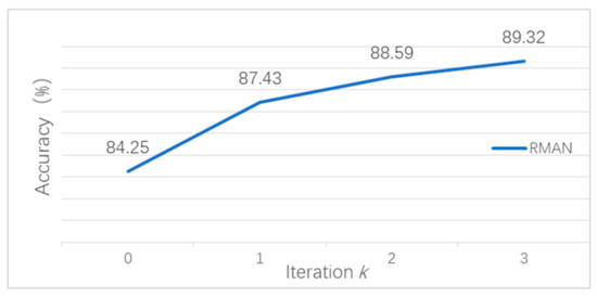
Figure 7.
Classification accuracy with a different number of iterations on the Scene 30 dataset.
In order to further evaluate the classification performance of the RMAN model on an indoor scene, we conducted experiments on the public dataset MIT Indoor 67. The experimental configuration parameters are shown in Section 4.2. Table 2 shows the classification accuracy of different approaches on MIT Indoor 67. It can be seen that MIT Indoor 67, as an indoor scene dataset, increases the difficulty of scene classification. The classification results of state-of-the-art approaches are below 80%. However, the proposed RMAN model can achieve a classification accuracy above 80%, which exceeds any state-of-the-art approaches. For example, compared with VGG-16, as can be seen from the table, the accuracy of scene recognition of the RMAN model has been increased from 75.67% to 80.60% by the recurrent attention mechanism. The accuracy of the RMAN model with SVM classifier is 81.0%, with an increase of 0.4% compared to the RMAN model with SoftMax logistic regression classifier. We analyze that in the RMAN model, the training dataset is still not big enough for the SoftMax logistic regression classifier, as it is difficult for a small training dataset to bring better classification results for a complex recurrent memory attention network. In contrast, SVM trains the classifier through marginal samples, which can be considered as the subset of the training dataset, therefore, the problem of inadequate training samples for the SoftMax logistic regression classifier may not be so serious for the SVM classifier.
Table 2.
Comparison of Recurrent Memorized Attention Network (RMAN) with other methods on MIT Indoor 67.
In order to evaluate the performance of our proposed RMAN model on the large-scale scene recognition dataset, we conducted experiments on the public dataset SUN-397. The experimental configuration parameters are same as the parameters applied for the experiment on the dataset MIT Indoor 67. As Table 3 shows, our proposed RMAN model can achieve the highest classification accuracy on the large-scale scene dataset, surpassing traditional or state-of-the-art approaches. It is probably due to the proposed recurrently memorizing mechanism for providing more spatial layout patterns, which can improve the scene recognition accuracy.
Table 3.
Comparison of RMAN with other methods on SUN-397.
By analyzing the classification performance on the Scene 30, MIT Indoor 67, and SUN 397 datasets, we can see the effectiveness of the RMAN model proposed in this paper. Under the weak supervision using only image tags, end-to-end scene recognition is achieved. At the same time, the classification accuracy of the model is better than many state-of-the-art image scene classification models, and it is more suitable for real-world applications.
5. Conclusions
This paper introduces an image scene classification approach based on a recurrent memory attention mechanism, and we propose a new end-to-end scene recognition model, the so-called RMAN model, which includes a feature extraction module, attention localization module, and recurrent memory attention module. We explain in detail how the RMAN model recurrently performs attention area localization and memorizes the features of the essential scene objects in an image. Finally, in order to verify the effectiveness of the proposed model, we perform experiments on the construction dataset Scene 30 and the two public scene datasets, MIT Indoor 67 and SUN397. The experimental results report that the RMAN model has achieved better classification performance, surpassing state-of-the-art image scene recognition approaches.
There are several possible directions for improving our work. First, the framework of extracting scene features needs to be further investigated. In the scene image recognition task, the training data are generally insufficient, while the aims of scene recognition are complex and diverse; sometimes, the intra-class differences are obvious; sometimes, the inter-class similarities are high. Therefore, how to design a suitable framework to extract suitable scene features will be a meaningful and important area of research. Second, the object feature fusion scheme needs to be improved, as it plays an important role in the classification task. Therefore, how to design a better object feature fusion method that extracts the effective part of each feature and removes redundancy will also be an important research direction.
Author Contributions
X.S. and B.B. conceived and designed the experiments; X.Z. performed the experiments; G.T. analyzed the data; X.S. wrote the paper. All authors have read and agreed to the published version of the manuscript.
Funding
This work is supported by the National Nature Science Foundation of China under Grants (No. 61872199, No. 61872424 and No. 61936005), National Key Research and Development Project (No. 2020AAA0106200), Open Projects Program of National Laboratory of Pattern Recognition and Nanjing University of Posts and Telecommunications Support Funding (Grant No. NY218001).
Conflicts of Interest
The authors declare no conflict of interest.
References
- Zhou, B.; Lapedriza, A.; Xiao, J.; Torralba, A.; Oliva, A. Learning deep features for scene recognition using places database. In Advances in Neural Information Processing Systems; The MIT Press: Cambridge, MA, USA, 2014; pp. 487–495. [Google Scholar]
- Xiao, J.; Hays, J.; Ehinger, K.A.; Oliva, A.; Torralba, A. Sun database: Large-scale scene recognition from abbey to zoo. In Proceedings of the IEEE Computer Society Conference on Computer Vision and Pattern Recognition, San Francisco, CA, USA, 13–18 June 2010; pp. 3485–3492. [Google Scholar]
- Quattoni, A.; Torralba, A. Recognizing indoor scenes. In Proceedings of the IEEE Conference on Computer Vision and Pattern Recognition, Miami, FL, USA, 20–25 June 2009; pp. 413–420. [Google Scholar]
- Oliva, A.; Torralba, A. Modeling the shape of the scene: A holistic representation of the spatial envelope. Int. J. Comput. Vis. 2001, 42, 145–175. [Google Scholar] [CrossRef]
- Margolin, R.; Zelnik-Manor, L.; Tal, A. Otc: A novel local descriptor for scene classification. In European Conference on Computer Vision; Springer: Cham, Switzerland, 2014; pp. 377–391. [Google Scholar]
- Wu, J.; Rehg, J.M. Centrist: A visual descriptor for scene categorization. IEEE Trans. Pattern Anal. Mach. Intell. 2010, 33, 1489–1501. [Google Scholar]
- Xiao, Y.; Wu, J.; Yuan, J. mCENTRIST: A multi-channel feature generation mechanism for scene categorization. IEEE Trans. Image Process. 2013, 23, 823–836. [Google Scholar] [CrossRef] [PubMed]
- LeCun, Y.; Bottou, L.; Bengio, Y.; Haffner, P. Gradient-based learning applied to document recognition. Proc. IEEE 1998, 86, 2278–2324. [Google Scholar] [CrossRef]
- Russakovsky, O.; Deng, J.; Su, H.; Krause, J.; Satheesh, S.; Ma, S.; Huang, Z.; Karpathy, A.; Khosla, A.; Bernstein, M.; et al. Imagenet large scale visual recognition challenge. Int. J. Comput. Vis. 2015, 115, 211–252. [Google Scholar] [CrossRef]
- Krizhevsky, A.; Sutskever, I.; Hinton, G.E. Imagenet classification with deep convolutional neural networks. In Advances in Neural Information Processing Systems; The MIT Press: Cambridge, MA, USA, 2012; pp. 1097–1105. [Google Scholar]
- Simonyan, K.; Zisserman, A. Very deep convolutional networks for large-scale image recognition. arXiv 2014, arXiv:1409.1556. [Google Scholar]
- Szegedy, C.; Liu, W.; Jia, Y.; Sermanet, P.; Reed, S.; Anguelov, D.; Erhan, D.; Vanhoucke, V.; Rabinovich, A. Going deeper with convolutions. In Proceedings of the IEEE Conference on Computer Vision and Pattern Recognition, Boston, MA, USA, 7–12 June 2015; pp. 1–9. [Google Scholar]
- He, K.; Zhang, X.; Ren, S.; Sun, J. Deep residual learning for image recognition. In Proceedings of the IEEE Conference on Computer Vision and Pattern Recognition, Las Vegas, NV, USA, 27–30 June 2016; pp. 770–778. [Google Scholar]
- Huang, G.; Liu, Z.; Van Der Maaten, L.; Weinberger, K.Q. Densely connected convolutional networks. In Proceedings of the IEEE Conference on Computer Vision and Pattern Recognition, Honolulu, HI, USA, 21–26 July 2017; pp. 4700–4708. [Google Scholar]
- Lafferty, J.; McCallum, A.; Pereira, F.C.N. Conditional Random Fields: Probabilistic Models for Segmenting and Labeling Sequence Data; Morgan Kaufmann: San Francisco, CA, USA, 2001. [Google Scholar]
- Stamp, M. A Revealing Introduction to Hidden Markov Models; Department of Computer Science San Jose State University: San Jose, CA, USA, 2004; pp. 26–56. [Google Scholar]
- Geman, S.; Graffigne, C. Markov random field image models and their applications to computer vision. In Proceedings of the International Congress of Mathematicians, Berkeley, CA, USA, 3–11 August 1986; Volume 1, p. 2. [Google Scholar]
- Blei, D.M.; Ng, A.Y.; Jordan, M.I. Latent dirichlet allocation. J. Mach. Learn. Res. 2003, 3, 993–1022. [Google Scholar]
- Othman, K.M.; Rad, A.B. An indoor room classification system for social robots via integration of cnn and ecoc. Appl. Sci. 2019, 9, 470. [Google Scholar] [CrossRef]
- Chen, P.H.; Lin, C.J.; Schölkopf, B. A tutorial on ν-support vector machines. Appl. Stoch. Models Bus. Ind. 2005, 21, 111–136. [Google Scholar] [CrossRef]
- Rafiq, M.; Rafiq, G.; Agyeman, R.; Jin, S.I.; Choi, G.S. Scene classification for sports video summarization using transfer learning. Sensors 2020, 20, 1702. [Google Scholar] [CrossRef]
- Li, L.J.; Socher, R.; Fei-Fei, L. Towards total scene understanding: Classification, annotation and segmentation in an automatic framework. In Proceedings of the IEEE Conference on Computer Vision and Pattern Recognition, Miami, FL, USA, 20–25 June 2009; pp. 2036–2043. [Google Scholar]
- Sudderth, E.B.; Torralba, A.; Freeman, W.T.; Willsky, A.S. Learning hierarchical models of scenes, objects, and parts. In Proceedings of the Tenth IEEE International Conference on Computer Vision (ICCV 05), Beijing, China, 17–21 October 2005; Volume 1, pp. 1331–1338. [Google Scholar]
- Choi, M.J.; Lim, J.J.; Torralba, A.; Willsky, A.S. Exploiting hierarchical context on a large database of object categories. In Proceedings of the IEEE Computer Society Conference on Computer Vision and Pattern Recognition, San Francisco, CA, USA, 13–18 June 2010; pp. 129–136. [Google Scholar]
- Li, C.; Parikh, D.; Chen, T. Automatic discovery of groups of objects for scene understanding. In Proceedings of the IEEE Conference on Computer Vision and Pattern Recognition, Providence, RI, USA, 16–21 June 2012; pp. 2735–2742. [Google Scholar]
- Wu, R.; Wang, B.; Wang, W.; Yu, Y. Harvesting discriminative meta objects with deep CNN features for scene classification. In Proceedings of the IEEE International Conference on Computer Vision, Santiago, Chile, 7–13 December 2015; pp. 1287–1295. [Google Scholar]
- Cheng, X.; Lu, J.; Feng, J.; Yuan, B.; Zhou, J. Scene recognition with objectness. Pattern Recognit. 2018, 74, 474–487. [Google Scholar] [CrossRef]
- Shao, X.; Zhang, J.; Bao, B.K.; Xia, Y. Automatic scene recognition based on constructed knowledge space learning. IEEE Access 2019, 7, 102902–102910. [Google Scholar] [CrossRef]
- Shi, J.; Zhu, H.; Yu, S.; Wu, W.; Shi, H. Scene categorization model using deep visually sensitive features. IEEE Access 2019, 7, 45230–45239. [Google Scholar] [CrossRef]
- Yin, W.; Ebert, S.; Schütze, H. Attention-based convolutional neural network for machine comprehension. arXiv 2016, arXiv:1602.04341. [Google Scholar]
- Yang, Z.; Yang, D.; Dyer, C.; He, X.; Smola, A.; Hovy, E. Hierarchical attention networks for document classification. In Proceedings of the Conference of the North American Chapter of the Association for Computational Linguistics: Human Language Technologies, San Diego, CA, USA, 12–17 June 2016; pp. 1480–1489. [Google Scholar]
- Vaswani, A.; Shazeer, N.; Parmar, N.; Uszkoreit, J.; Jones, L.; Gomez, A.N.; Kaiser, Ł.; Polosukhin, I. Attention is all you need. In Advances in Neural Information Processing Systems; The MIT Press: Cambridge, MA, USA, 2017; pp. 5998–6008. [Google Scholar]
- Lin, D.; Shen, X.; Lu, C.; Jia, J. Deep lac: Deep localization, alignment and classification for fine-grained recognition. In Proceedings of the IEEE Conference on Computer Vision and Pattern Recognition, Boston, MA, USA, 7–12 June 2015; pp. 1666–1674. [Google Scholar]
- Liu, X.; Xia, T.; Wang, J.; Yang, Y.; Zhou, F.; Lin, Y. Fully convolutional attention networks for fine-grained recognition. arXiv 2016, arXiv:1603.06765. [Google Scholar]
- Zheng, H.; Fu, J.; Mei, T.; Luo, J. Learning multi-attention convolutional neural network for fine-grained image recognition. In Proceedings of the IEEE international Conference on Computer Vision, Venice, Italy, 22–29 October 2017; pp. 5209–5217. [Google Scholar]
- Ren, S.; He, K.; Girshick, R.; Sun, J. Faster r-cnn: Towards real-time object detection with region proposal networks. In Advances in Neural Information Processing Systems; The MIT Press: Cambridge, MA, USA, 2015; pp. 91–99. [Google Scholar]
- Jaderberg, M.; Simonyan, K.; Zisserman, A. Spatial transformer networks. In Advances in Neural Information Processing Systems; The MIT Press: Cambridge, MA, USA, 2015; pp. 2017–2025. [Google Scholar]
- Xue, X.; Zhang, W.; Zhang, J.; Wu, B.; Fan, J.; Lu, Y. Correlative multi-label multi-instance image annotation. In Proceedings of the IEEE International Conference on Computer Vision, Barcelona, Spain, 6–13 November 2011; pp. 651–658. [Google Scholar]
- Wang, J.; Yang, Y.; Mao, J.; Huang, Z.; Huang, C.; Xu, W. Cnn-rnn: A unified framework for multi-label image classification. In Proceedings of the IEEE Conference on Computer Vision and Pattern Recognition, Las Vegas, NV, USA, 27–30 June 2016; pp. 2285–2294. [Google Scholar]
- Krishna, R.; Zhu, Y.; Groth, O.; Johnson, J.; Hata, K.; Kravitz, J.; Chen, S.; Kalantidis, Y.; Li, L.J.; Shamma, D.A.; et al. Visual genome: Connecting language and vision using crowdsourced dense image annotations. Int. J. Comput. Vis. 2017, 123, 32–73. [Google Scholar] [CrossRef]
- Glorot, X.; Bengio, Y. Understanding the difficulty of training deep feedforward neural networks. In Proceedings of the Thirteenth International Conference on Artificial Intelligence and Statistics, Sardinia, Italy, 13–15 May 2010; pp. 249–256. [Google Scholar]
- Chollet, F. Keras. Available online: https://github.com/keras-team/keras (accessed on 20 October 2020).
- Juneja, M.; Vedaldi, A.; Jawahar, C.V.; Zisserman, A. Blocks that shout: Distinctive parts for scene classification. In Proceedings of the IEEE Conference on Computer Vision and Pattern Recognition, Portland, OR, USA, 23–28 June 2013; pp. 923–930. [Google Scholar]
- Lin, D.; Lu, C.; Liao, R.; Jia, J. Learning important spatial pooling regions for scene classification. In Proceedings of the IEEE Conference on Computer Vision and Pattern Recognition, Columbus, OH, USA, 23–28 June 2014; pp. 3726–3733. [Google Scholar]
- Gong, Y.; Wang, L.; Guo, R.; Lazebnik, S. Multi-scale orderless pooling of deep convolutional activation features. In European Conference on Computer Vision; Springer: Cham, Switzerland, 2014; pp. 392–407. [Google Scholar]
- Sharif Razavian, A.; Azizpour, H.; Sullivan, J.; Carlsson, S. CNN features off-the-shelf: An astounding baseline for recognition. In Proceedings of the IEEE Conference on Computer Vision and Pattern Recognition Workshops, Columbus, OH, USA, 23–28 June 2014; pp. 806–813. [Google Scholar]
- Zuo, Z.; Wang, G.; Shuai, B.; Zhao, L.; Yang, Q.; Jiang, X. Learning discriminative and shareable features for scene classification. In European Conference on Computer Vision; Springer: Cham, Switzerland, 2014; pp. 552–568. [Google Scholar]


Publisher’s Note: MDPI stays neutral with regard to jurisdictional claims in published maps and institutional affiliations. |
© 2020 by the authors. Licensee MDPI, Basel, Switzerland. This article is an open access article distributed under the terms and conditions of the Creative Commons Attribution (CC BY) license (http://creativecommons.org/licenses/by/4.0/).