PV Module Fault Detection Using Combined Artificial Neural Network and Sugeno Fuzzy Logic

Abstract

This work introduces a new fault detection method for photovoltaic systems. The method identifies short-circuited modules and disconnected strings on photovoltaic systems combining two machine learning techniques. The first algorithm is a multilayer feedforward neural network, which uses irradiance, ambient temperature, and power at the maximum power point as input variables. The neural network output enters a Sugeno type fuzzy logic system that precisely determines how many faulty modules are occurring on the power plant. The proposed method was trained using a simulated dataset and validated using experimental data. The obtained results showed 99.28% accuracy on detecting short-circuited photovoltaic modules and 99.43% on detecting disconnected strings.

1. Introduction

Photovoltaic (PV) solar energy has been showing worldwide expansion, reaching an installed capacity of 627 GW [1]. Following this growth, it is essential to ensure the security and reliability of solar power plants. In this perspective, some challenging issues are associated with it, such as faults occurring on PV systems, that may impact the secure operation and the optimal energy harvesting.

The reliability of the PV system can be affected by several factors, such as weather conditions, partial shading, dust/snow accumulation on the modules, wiring losses, aging or malfunctioning of any system component [2]. Some faults could remain undetected by the operators for long periods, and it has the potential to reduce 18.9% of power production [3]. Therefore, it is essential to develop methods capable of detecting and diagnosing fault occurrence in PV systems.

Faults in PV systems can arise on the Direct Current (DC) or the Alternate Current (AC) side. It can affect the PV modules, converters, Maximum Power Point Tracking (MPPT), and storage system on the DC side. PV modules faults are crucial since it is the generation unit of a PV system. Faults occurring on this device could significantly affect the output power. In addition, it could have destructive effects on their efficiency and lifetime [2].

There are various PV module fault sources, such as mismatch, bypass diode, circuit faults, asymmetrical faults, arc faults, ground faults, and lightning. It can be temporary or permanent, depending on the cause and the period that affects the PV systems performance [4]. The circuit faults, which are the subject of this research, can be open-circuit or short-circuit. In both situations, the PV module does not contribute to power generation, so it could significantly decrease the system performance and remain undetected.

Therefore, some monitoring and diagnosis techniques have been developed in recent years. Diagnosis methods can be classified into two general groups: visual and electric. Visual methods require constant verification by an operator and some specific types of equipment. On the other hand, electrical methods use output signals such as voltage, current, and power to identify fault occurrence [5]. Furthermore, it is possible to use existing sensors and pieces of equipment, making it more viable for implementing the fault detection method.

In this context, researchers have been exploring different techniques for detecting and diagnosing faults on PV systems. Methods which apply machine learning are widely explored since it offers an alternative way for approaching complex issues. Some of these methods explore detecting the fault in advance, predictively, avoiding massive power losses and damages on PV systems [6]. However, the most common methods search for fault diagnosis in real-time.

Syafaruddin et al. [7] developed a diagnosis method using an artificial neural network (ANN). In this case, one neural net was trained for each PV module in order to identify and locate short-circuited modules. The input variables are module temperature, irradiance, and maximum power point voltage and current. The method showed promising results, although it was tested only for a six modules PV system.

Li et al. [8] also applied ANN for fault detection, using the same inputs as [7]. For training, the dataset used was extracted from simulations using MATLAB/Simulink^®. The faults detected by the method are degradation, short-circuited modules, and partial shading. However, the method was not experimentally tested. Jiang and Maskell [9] developed a technique for detection combining ANN and an analytical method. The ANN forecasts the maximum power point (MPP), using module temperature and irradiance as inputs. The algorithm identifies the fault comparing the provided MPP to the one measured. The faults approached in this method are open-circuited string/module, short-circuited module, partial shading, and malfunctioning MPPT. However, the authors did not test the method experimentally.

Akram and Lotfifard [10] trained a Probabilistic Neural Network (PNN) for detecting short-circuited and open-circuited modules on PV systems. The dataset for training the neural network was assembled by simulation using MATLAB/Simulink^® software, and its test showed a maximum error of 3.5%. Nevertheless, it was not tested experimentally, only with simulation data. Furthermore, Garoudja et al. [11] also developed a fault detection method using a PNN. Firstly, the PV module parameters are extracted in order to simulate the studied PV system. The simulation is performed using MATLAB/Simulink^® and PSIM^® and validated with experimental data. They trained the neural network using the simulated dataset, and the input variables are module temperature, irradiance, and voltage and current at the MPP. This approach detected short-circuited modules and string disconnections. The authors tested the method experimentally and compared the performance of an ANN and a PNN. The results showed an accuracy of 90.3% for the ANN and 100% for the PNN.

Chine et al. [12] created a method that combines two algorithms. The first one compares the measured output power to the simulated-on MATLAB/Simulink^® software. If the difference is more significant than the stipulated threshold, the algorithm identifies faults presence, and the signal enters the ANN. The Radial Basis Function (RBF) neural network was trained with a simulated dataset and diagnosis faults on bypass diodes, short-circuit and open-circuit modules, and partial shading. This method was experimentally tested by the authors and showed good accuracy.

Dhimish et al. [13,14] developed a fault detection for partial shading and short-circuited modules using a multilayer algorithm. The first layers use LabVIEW^® simulations and third-order polynomial function modelling. The last layer uses a fuzzy classifier to diagnose the fault type occurring on the PV system. The method was tested using experimental data, and its results showed an accuracy of 95.27% with the fuzzy layer and 98.8% with the fuzzy layer.

Dhimish et al. [15] compared a fuzzy logic system to an ANN for partial shading, short-circuited module, and malfunctioning MPPT fault detection. The authors trained the RBF neural network using a voltage and power ratio, and the same variables were used to implement the Mamdani and Sugeno fuzzy logic systems. The voltage ratio and power ratio were calculated, considering simulation results performed using MATLAB/Simulink^®. The findings showed a superior accuracy of the ANN, reaching 92.1%.

Hussain et al. [16] compared two different ANNs for developing a fault detection method. The neural networks used were RBF and Multilayer Perceptron (MLP) for detecting disconnected PV modules on a string. The input variables were power and irradiance, and the output indicates how many faulty modules are on the string. Results showed a maximum accuracy of 97.9% on the RBF neural network.

Considering the previous discussion, it is essential to develop methods capable of identifying and diagnosing the PV system’s fault. Therefore, this paper proposes a fault detection technique combining ANN and fuzzy logic to detect short-circuited modules and disconnected strings on a PV power plant. It is essential to detect this fault type since it can massively decrease power generation, and identifying it can be time-consuming, especially on large scale power plants.

A notable advantage of this work is that the proposed method is suitable and reliable once it uses pre-existing sensors, and the training dataset is obtained by simulation, not requiring long data from an existing PV system. In addition, the method does not need to compare simulated results with measured data, making it more straightforward.

The paper is briefly structured as follows. Section 2 illustrates the modelling of the PV module and explains mathematical equations needed for PV system simulation. Then, Section 3 describes the studied PV systems in this research, and also validates the model simulation using experimental data. Section 4 defines the methodology used to develop the fault detection method. In Section 5, the proposed method is validated with an experimental dataset of the studied PV systems. Finally, in Section 6, the overall conclusions are discussed.

2. PV Module Modelling

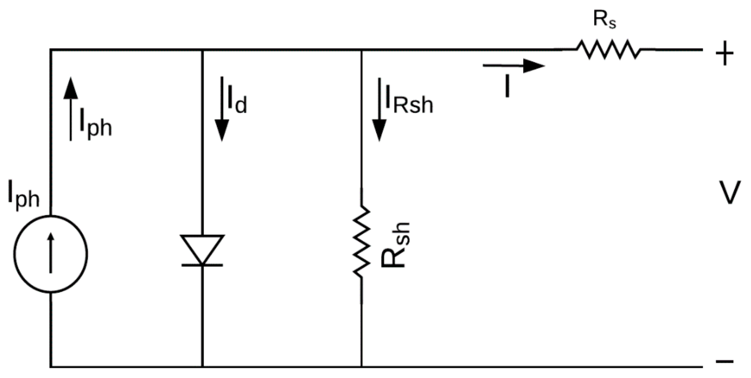
Several PV cell models are proposed in the literature [17], but for this work, the one diode model was employed, considering its simplicity. Figure 1 illustrates the equivalent circuit for the one diode model.

The circuit comprises the light-generated current (I_ph), parallel with a diode and a shunt resistance (R_sh). All these elements are series-connected to the series resistance (R_s). Analysing the circuit in Figure 1, the cell output current I can be expressed by Equation (1).

$$\mathrm{I}={\mathrm{I}}_{\mathrm{ph}}-{\mathrm{I}}_{\mathrm{d}}-{\mathrm{I}}_{\mathrm{Rsh}}$$

(1)

The I_d and I_Rsh currents represent the diode current and leakage current, respectively, and are expressed by Equations (2) and (3).

$${\mathrm{I}}_{\mathrm{d}}={\mathrm{I}}_0\left[\exp \left(\frac{{\mathrm{V}}_{\mathrm{d}}\mathrm{q}}{\mathrm{akT}}\right)-1\right]$$

(2)

$${\mathrm{I}}_{\mathrm{Rsh}}=\frac{\mathrm{V}+{\mathrm{R}}_{\mathrm{s}}\mathrm{I}}{{\mathrm{R}}_{\mathrm{sh}}}$$

(3)

Substituting the I_d and I_Rsh expression on Equation (1), the current I delivered by the PV cell is represented on Equation (4).

$$\mathrm{I}={\mathrm{I}}_{\mathrm{ph}}-{\mathrm{I}}_0\left[\exp \left(\frac{{\mathrm{V}}_{\mathrm{d}}\mathrm{q}}{\mathrm{akT}}\right)-1\right]-\frac{\mathrm{V}+{\mathrm{R}}_{\mathrm{s}}\mathrm{I}}{{\mathrm{R}}_{\mathrm{sh}}}$$

(4)

where:

I₀

Diode saturation current (A);

V_d

Diode voltage (V);

q

Electron charge ($q=1.6\times {10}^{-19}\mathrm{C}$);

a

Diode ideality factor;

k

Boltzmann constant ($k=1.38\times {10}^{-23}\mathrm{J}/\mathrm{K}$);

V

Cell output voltage (V);

T

T Cell operating temperature (K);

R_s

Series resistance (Ω);

R_sh

Shunt resistance (Ω).

The light generated current I_ph of a PV cell depends on the irradiance and the cell operating temperature expressed by Equations (5) and (6).

$${\mathrm{I}}_{\mathrm{ph}}=\left[{\mathrm{I}}_{\mathrm{phn}}+{\mathrm{k}}_{\mathrm{i}}\left(\mathrm{T}-{\mathrm{T}}_{\mathrm{n}}\right)\right]\frac{\mathrm{G}}{{\mathrm{G}}_{\mathrm{n}}}$$

(5)

$${\mathrm{I}}_{\mathrm{phn}}=\frac{{\mathrm{R}}_{\mathrm{sh}}+{\mathrm{R}}_{\mathrm{s}}}{{\mathrm{R}}_{\mathrm{sh}}}{\mathrm{I}}_{\mathrm{sc}}$$

(6)

where:

I_phn

Nominal light generated current (A);

I_sc

Short-circuit current for STC (Standard Test Conditions) (A);

k_i

Temperature coefficient for I_sc (A/K);

T_n

Cell temperature for STC (298 K);

G

Cell irradiance (W/m²);

G_n

Cell irradiance for STC (1000 W/m²).

The diode saturation current I₀ is related to the cell operating temperature and is expressed by Equation (7).

$${\mathrm{I}}_0={\mathrm{I}}_{0\mathrm{n}}{\left(\frac{{\mathrm{T}}_{\mathrm{n}}}{\mathrm{T}}\right)}^3\exp \left[\frac{{\mathrm{qE}}_{\mathrm{g}0}}{\mathrm{ak}}\left(\frac{1}{{\mathrm{T}}_{\mathrm{n}}}-\frac{1}{\mathrm{T}}\right)\right]$$

(7)

E_g0 is the bandgap energy for semiconductor and is 1.2 eV to the polycrystalline siliceous at 25 °C [18], and the I_0n is the nominal saturation current, expressed by Equation (8).

$${\mathrm{I}}_{0\mathrm{n}}=\frac{{\mathrm{I}}_{\mathrm{sc}}+{\mathrm{k}}_{\mathrm{i}}\left(\mathrm{T}-{\mathrm{T}}_{\mathrm{n}}\right)}{\exp \left\{\frac{\mathrm{q}\left[{\mathrm{V}}_{\mathrm{oc}}+{\mathrm{k}}_{\mathrm{v}}\left(\mathrm{T}-{\mathrm{T}}_{\mathrm{n}}\right)\right]}{{\mathrm{akT}}_{\mathrm{n}}}\right\}-1}$$

(8)

V_oc is the cell’s open-circuit voltage, and k_v temperature coefficient for V_oc expressed in V/K. Finally, analysing the circuit in Figure 1, the diode voltage (V_d) can be represented by Equation (9).

$${\mathrm{V}}_{\mathrm{d}}= \mathrm{V}+{\mathrm{R}}_{\mathrm{s}}\mathrm{I}$$

(9)

The one diode model characterized by Figure 1 and Equation (4) represents one single PV cell. However, in practice, a PV module comprises several connected PV cells, and a PV array comprises several connected PV modules. Thus, to analyse the I and V output characteristics of an entire PV module/array, it is necessary to include the parameters of the number of series-connected cells (N_s) and parallel-connected cells (N_p), as expressed by Equations (10) and (11).

$$\mathrm{I}={\mathrm{N}}_{\mathrm{P}}{\mathrm{I}}_{\mathrm{ph}}-{\mathrm{N}}_{\mathrm{P}}{\mathrm{I}}_0\left[\exp \left(\frac{\mathrm{q}\left(\mathrm{V}+{\mathrm{R}}_{\mathrm{s}}\mathrm{I}\right)}{{\mathrm{N}}_{\mathrm{s}}\mathrm{akT}}\right)-1\right]-\frac{\mathrm{V}+{\mathrm{R}}_{\mathrm{s}}\mathrm{I}}{{\mathrm{R}}_{\mathrm{sh}}}$$

(10)

$${\mathrm{I}}_{0\mathrm{n}}=\frac{{\mathrm{I}}_{\mathrm{sc}}+{\mathrm{k}}_{\mathrm{i}}\left(\mathrm{T}-{\mathrm{T}}_{\mathrm{n}}\right)}{\exp \left\{\frac{\mathrm{q}\left[{\mathrm{V}}_{\mathrm{oc}}+{\mathrm{k}}_{\mathrm{v}}\left(\mathrm{T}-{\mathrm{T}}_{\mathrm{n}}\right)\right]}{{\mathrm{N}}_{\mathrm{s}}{\mathrm{akT}}_{\mathrm{n}}}\right\}-1}$$

(11)

It is essential to highlight that when analysing a PV module/array, R_s and R_sh are the equivalent resistance. In addition, V_oc and I_sc value the whole PV module/array for the Standard Test Conditions (STC). Moreover, the temperature T corresponds to the cell operating temperature, not the ambient temperature. When it is not available the cell or module temperature (T_c), it is possible to assume that T is dependent on the ambient temperature (T_a) and the Nominal Operating Cell Temperature (NOCT), as expressed by Equation (12) [19].

$${\mathrm{T}}_{\mathrm{c}}={\mathrm{T}}_{\mathrm{a}}+\frac{\mathrm{G}}{800}\left(\mathrm{NOCT}-20\right)$$

(12)

Considering the model and expressions analysed, the subsection describes PV system modelling on MATLAB/Simulink^® software.

MATLAB Simulink^® Simulation

The PV module modelling was developed using the one diode model in the MATLAB/Simulink^® environment, as shown in Figure 2.

In Figure 2, the grey blocks are input variables, the pink blocks are the outputs of the PV modules, the yellow blocks are constants, and the blue blocks are masks containing previously discussed equations. Moreover, to avoid a loop error, a low pass filter was employed (see the green block in Figure 2) as a feedback transfer function, and C is the filter time constant. The filter discretizes the model solution, enabling it to solve the equation and store the correct results. The time constant C should increase with the number of cells. Thus, there will be enough time for the algorithm to solve the equation, store the result, and perform the next iteration.

The manufacturers provide most of the PV modules’ parameters. Generally, the parameters available on the panel datasheet are open-circuit voltage (V_oc), short-circuit current (I_sc), the Maximum Power Point (MPP) voltage (V_MPP), the current ate the MPP (I_MPP), and the power at MPP (P_MPP). Thus, according to Equations (10) and (11), the parameters that are not available on the PV module datasheet are the diode ideality factor (a), the series resistance (R_s), and the shunt resistance (R_sh). While some authors investigated how to estimate the ideality factor a [20,21], in the context of this work, it was considered 1 ≤ a ≤ 1.5 [18]. The ideality factor a was chosen to improve the model fitting. Furthermore, the model resistances R_s and R_sh were calculated according to Villalva’s method [18].

After modelling a PV module, it is possible to simulate an entire PV array, working under healthy or faulty conditions. The simulation enabled the development of the proposed method applied to the system described. Section 3 discusses the modelling validation.

3. Model Validation with Experimental Data

For the model validation, a comparison with experimental data is incredibly useful. It is essential to understand how the model works under different PV module models and different conditions. Thus, the proposed model was tested for two different PV systems, named here as System 1 and System 2. Section 3.1 and Section 3.2 describe the model validation for both systems.

3.1. System 1: One String System

The PV array named System 1 in this research is illustrated in Figure 3. The system is a 2.2 kWp PV power plant, and it comprises ten series-connected PV modules. The panels model is the SMT6(60)P from PowerGlaz manufacturer, installed at the Huddersfield University campus, and

Table 1. SMT6(60)P PV module parameters.

Datasheet Parameters
Parameter	Value	Parameter	Value
VOC	36.74 V	Ns	60
ISC	8.24 A	Np	1
ki	0.0042 A/K	PMPP	220 W
kV	−0.132 V/K	IMPP	7.7 A
NOCT	46 °C	VMPP	28.7 V
Calculated Parameters
Parameter	Value	Parameter	Value
Rsh (Ω)	1108.3972	Rs (Ω)	0.3930

describes its characteristics.

We simulated System 1 using the model proposed in Section 2. Then, we compared the model simulation results to measured experimental data. We observed the model results varying the irradiance G. Figure 4 illustrates the P-V (Power vs. Voltage) curves, comparing to the experimental data.

Observing Figure 4, it is possible to verify that the proposed model shows results consistent with the measured P_MPP for the experimented system.

Table 2. System 1 experimental results.

Ta (°C)	G (W/m2)	Measured PMPP (W)	Model Simulation PMPP (W)	Error (%)
16	88	185.26	186.30	0.56
16	110	238.15	236.00	−0.90
16	224	493.00	487.90	−1.03
16	329	709.11	707.20	−0.27

summarizes a comparison of measurements of System 1 and simulation results.

After verifying the proposed model accuracy, we performed simulations to build the fault detection method’s training database. A large dataset for the machine learning training is necessary to simulate faulty scenarios and healthy scenarios, varying the irradiance level and the module temperature. In system 1, the fault detection method is supposed to diagnose short-circuited PV modules. Thus, we simulated ten scenarios, disconnecting 1, 2, 3, until 9 modules. In each scenario, the irradiance was wide-ranging from 100 W/m² to 1100 W/m², and the ambient temperature from 10 °C to 40 °C. In addition, the P_MPP was measured for each case.

3.2. System 2: Four String System

The second PV system studied in this research, called System 2, is illustrated in Figure 5. The PV system is a 4.16 kW_p power plant and comprises 32 PV modules, arranged on four series-connected strings, with eight series-connected modules on each string. The panels model is the KC130GHT-2 from Kyocera manufacturer, also installed at the Huddersfield University campus, and

Table 3. KC130GHT-2 PV module parameters.

Datasheet Parameters
Parameter	Value	Parameter	Value
Voc	21.90 V	Ns	36
Isc	8.02 A	Np	1
ki	0.00318 A/K	PMPP	130 W
kv	−0.0821 V/K	IMPP	7.39 A
NOCT	47 °C	VMPP	17.6 V
Calculated Parameters
Parameter	Value	Parameter	Value
Rp (Ω)	119.232	Rs (Ω)	0.16

describes its characteristics.

We also simulated System 2 using the model proposed in Section 2. Following the same previous methodology, we compared the model simulation results to measured experimental data. We observed the model results varying the irradiance G. Figure 6 illustrates the P-V curves for System 2, comparing it to the experimental data.

Observing Figure 6, it is possible to verify that the proposed model shows results consistent with the measured P_MPP for the experimented system.

Table 4. System 1 experimental results.

Ta (°C)	G (W/m2)	Measured PMPP (W)	Model Simulation PMPP (W)	Error (%)
16	145	588.69	578.93	−1.66
16	254	1086.8	1080.75	0.56
16	300	1262.41	1286.00	−1.87
16	403	1701.63	1727.78	−1.54

summarizes a comparison of measurements of System 2 and simulation results.

After verifying the proposed model accuracy, we performed simulations to build the fault detection method’s training database. In System 2, the fault detection method is supposed to diagnose strings disconnection fault. Thus, we modelled four scenarios, disconnecting 1, 2, and 3 strings. In each scenario, the irradiance was wide-ranging from 100 W/m² to 1100 W/m², and the ambient temperature from 10 °C to 40 °C. Furthermore, the P_MPP was measured for each case. With the simulated dataset, it is possible to develop the fault detection method for System 1 and 2, discussed in Section 4.

4. Fault Detection Method

The proposed fault detection method identifies short-circuited modules on System 1 and disconnected strings on System 2, indicating how many PV modules or strings are under the faulty condition. The input variables should be the irradiance (G), ambient temperature (Ta), and the measured power at the MPP (P_MPP). The only electrical variable, in this case, is the P_MPP, which makes the fault detection quite tricky. The same output power could represent various situations, including healthy and faulty conditions. Figure 7 compares two P–V curves of System 1 under different conditions to exemplify this situation.

Observing Figure 7, we can see that even under entirely different conditions, the measured P_MPP could be quite similar. Therefore, any fault detection method needs to deal with this similarity on the database, mostly if it uses only the maximum power point (P_MPP) as electrical variable. Seeking to deal with this issue, we proposed combining two algorithms, as illustrated in Figure 8.

The first algorithm is an ANN using as input variables the irradiance G, the module temperature T_c, and the measured power at the MPP (P_MPP). The neural network output enters a fuzzy logic classifier that detects how many PV modules are under short-circuit fault or strings are disconnected. It is essential to highlight that the method’s objective is to give the operator the exact number of short-circuited PV modules or disconnected strings on the system. Therefore, using a fuzzy classifier is essential to enable the method to deal with the similarities in the output power and still give the correct number of faults occurring on the PV system.

Table 5. Faults indicated by the detection method.

	Short-Circuited PV Modules	Fault	Output
System 1	0	F0	0
	1	F1	1
	2	F2	2
	3	F3	3
	…	…	…
	9	F9	9
	Disconnected Strings	Fault	Output
System 2	0	F0	0
	1	F1	1
	2	F2	2
	3	F3	3

exemplifies the faults indicated by the detection method.

System 1 comprises ten panels, so if there are ten faulty PV modules, the entire system is disconnected. Therefore, this faulty condition does not correspond to short-circuited PV modules but system failure. So, observing Table 5, the proposed method identifies 0 (normal operation) to 9 short-circuited PV modules for System 1. The ANNs and fuzzy logic details for each system are described in Section 4.1 and Section 4.2.

4.1. Artificial Neural Network

The ANN of the fault detection method applied to the studied system is a Multilayer Perceptron (MLP) neural network. On an MLP network, each layer has a weight matrix W, a bias vector b, and an output vector Y, as illustrated in Figure 9, where f(.) is the used activation function. The outputs of the hidden layer are defined by Equations (13) and (14) [22].

$${}_{}{}^{1}Y={}_{}{}^{1}f\left({}_{}{}^{2}w\times X+{}_{}{}^{1}b\right)$$

(13)

$${}_{}{}^{2}Y={}_{}{}^{2}f\left({}_{}{}^{2}w\times {}_{}{}^{1}Y+{}_{}{}^{2}b\right)$$

(14)

In general, MLP networks can be applied to linear or nonlinear models. Usually, it is associated with sigmoid, tansigmoid, or linear activation functions. They are often used because they provide nonzero derivatives regarding input signals and exhibits smoothness and asymptotic properties. The linear activation function is employed to approximate a continuous function in the output layer of MLP networks. There is no formal rule for choosing the number of hidden layers of neurons on it, though the number of neurons in the hidden layer impacts the network performance. A large number of neurons in the hidden layers will make the training process slow [22].

We developed the MLP using MATLAB^® software. Figure 10 represents the structure of the MLP applied to the fault detection method, and

Table 6. System 1 and 2 MLP training settings.

Artificial Neural Network (ANN) Setup
Number of input variables	3 (G, T, PMPP)
Number of output variables	1
Number of layers	2
Number of neurons	(10, 1)
Training Process	Supervised
Training algorithm	Levenberg-Marquardt
Activation function	(tansigmoid, linear)
Training	70%
Validation	15%
Test	15%
Type of division of samples	random

describes its settings.

The training process was supervised, meaning that we provided a set of input/output data of appropriate network behaviour. We divided randomly 70% of the samples for training, 15% for validation, and 15% for testing. Thus, we enabled the validation of the desired topology. The training algorithm chosen is Levenberg-Marquardt, considering it is a faster algorithm for networks of moderate sizes.

The training dataset was obtained, as discussed in Section 3.1 and Section 3.2. For System 1, it comprises 147 samples for each simulated scenario, a total of 1470 samples. For System 2, the dataset comprises 588 samples and 147 samples for each simulated scenario. We compiled the samples in a crescent order of output power (P_MPP), along with the respective irradiance (G) and ambient temperature (T_a).

Hence, values varying from 0 to the number of possible faults occurring on the array for the targets were assumed. Therefore, for System 1, the targets assumed ranges from 0 to 9.99, with a step 0.0068 according to the number of samples on each scenario. Thus, in training, the algorithm can understand that even for the same P_MPP, it could represent more than one faulty situation.

For System 2, the targets assumed ranges from 0 to 3.99. For instance, if two faulty PV modules occur on System 1, the ANN targets vary from 2 to 2.99. It is worth highlighting that an ANN output of 2.9 is not more critical or closer to three faulty PV modules than a 2.4 result. Both output values mean that there are two short-circuited PV modules in the system (in the case of System 1). The range in the output values is necessary to avoid incorrect fault detection in those cases of output power (P_MPP) are too similar even in different conditions.

Thus, each fault condition corresponds to a range of outputs values on the ANN. The training process took six epochs for both ANNs. The regression coefficients are R1 = 0.99996 and R2 = 0.99848 for System 1 and System 2 ANNs, respectively. These coefficients mean that the trained networks’ outputs closely represent those used as training data.

The output signal is not an absolute number since each faulty condition corresponds to a range of output values, so the fuzzy logic system classifies and can determine precisely how many faults are occurring on the PV system [23].

4.2. Fuzzy Logic System

In this study, the second algorithm, combined with the ANN, is responsible for giving the operator the exact number of faulty conditions in a PV system. Considering that each faulty condition corresponds to a range of the ANN results, it could be simply trunked to the integer value by an algorithm. However, we observed that due to similarities in the P_MPP, as previously discussed in Section 4, the ANN output not always follows the expected linearity. So, in some cases, the ANN output values are out of the range for the given faulty condition.

Therefore, considering the ANN results, a fuzzy logic system interface can precisely determine how many faulty PV modules or disconnected strings are on the examined PV system since the operator can easily set the range of the membership functions.

The implemented fuzzy logic is a Sugeno type, developed on MATLAB^®, using the software’s default fuzzy inference rules. We chose the Takagi–Sugeno–Kang fuzzy inference system considering the linear relation between the inputs and outputs [24]. Figure 11 and

Table 7. Fuzzy logic classifier settings.

Fuzzy Logic System Setup	System 1	System 2
Name	Classifier	Classifier
Type	Sugeno	Sugeno
Inputs/Outputs	[1 1]	[1 1]
Number of Input Membership Functions	10	4
Number of Output Membership Functions	10	4
Number of Rules	10	4
And Method	prod	prod
Or Method	probor	probor
ImpMethod	prod	prod
AggMethod	sum	sum
DefuzzMethod	wtaver	wtaver
Input Labels	ANNoutput	ANNoutput
Output Labels	Fault	Fault
Input Range	[−1 10]	[−1 10]
Output Range	[0 1]	[0 1]
Input Membership Function Types	trimf, trapmf	trimf, trapmf
Output Membership Function Types	constant	constant

shows its characteristics.

The ANN output is not an absolute number, and it enters the fuzzy classifier as an input variable. The fuzzy inference system is responsible for giving the precise number of short-circuited PV modules for System 1 and disconnected strings for System 2. Therefore, the output membership functions are constants, and

Table 8. Fuzzy classifier input and output membership functions.

	Input Membership Functions		Output Membership Functions
	Labels	Parameters	Labels	Parameters
System 1	F0	[−1 −1 0 0.5]	Fault_0	[0 0 0 0]
	F1	[0.5 1 2]	Fault_1	[1 0 0 0]
	F2	[1.5 2 3]	Fault_2	[2 0 0 0]
	F3	[2.5 3 3.9]	Fault_3	[3 0 0 0]
	F4	[3.5 4 5]	Fault_4	[4 0 0 0]
	F5	[4.5 5 6]	Fault_5	[5 0 0 0]
	F6	[5.5 6 7]	Fault_6	[6 0 0 0]
	F7	[6.5 7 8]	Fault_7	[7 0 0 0]
	F8	[7.5 8 9]	Fault_8	[8 0 0 0]
	F9	[8.5 9 10 10]	Fault_9	[9 0 0 0]
System 2	F0	[−1 −1 0 0.5]	Fault_0	[0 0 0 0]
	F1	[0.5 1 2]	Fault_1	[1 0 0 0]
	F2	[1.5 2 3]	Fault_2	[2 0 0 0]
	F3	[2.5 3 3.9]	Fault_3	[3 0 0 0]

describes the input and output membership function (MF) settings.

The fuzzy logic system rules are based on IF/THEN statements [25]. For the proposed fuzzy classifier, the rules are briefly listed in

Table 9. Fuzzy classifier rules.

	Fuzzy Rules
System 1	1. If (ANNoutput is F0) then (Fault is Fault_0) (1)
	2. If (ANNoutput is F1) then (Fault is Fault_1) (1)
	3. If (ANNoutput is F2) then (Fault is Fault_2) (1)
	4. If (ANNoutput is F3) then (Fault is Fault_3) (1)
	5. If (ANNoutput is F4) then (Fault is Fault_4) (1)
	6. If (ANNoutput is F5) then (Fault is Fault_5) (1)
	7. If (ANNoutput is F6) then (Fault is Fault_6) (1)
	8. If (ANNoutput is F7) then (Fault is Fault_7) (1)
	9. If (ANNoutput is F8) then (Fault is Fault_8) (1)
	10. If (ANNoutput is F9) then (Fault is Fault_9) (1)
System 2	1. If (ANNoutput is F0) then (Fault is Fault_0) (1)
	2. If (ANNoutput is F1) then (Fault is Fault_1) (1)
	3. If (ANNoutput is F2) then (Fault is Fault_2) (1)
	4. If (ANNoutput is F3) then (Fault is Fault_3) (1)

.

After refining the algorithms, it is attainable to test the proposed method. The following section, Section 5, discusses the testing results with experimental data.

5. Results and Discussion

In order to evaluate the effectiveness of the proposed fault detection method, the same simulated scenarios were experimentally tested. Section 5.1 and Section 5.2 describe the experimental setup and the method validation for both systems.

5.1. System 1 Experimental Setup and Method Validation

As discussed in Section 3, the PV plant comprises ten series-connected modules. The PV modules were disconnected from the string, creating all ten simulated scenarios, exemplifying the experimental setup shown in Figure 12.

During the experiments, the PV modules were disconnected for the entire day to collect enough data for testing the method. However, in real situations, a faulty condition may occur not necessarily for the whole day, just for a period. The experimental tests were performed for two weeks. Figure 13 and Figure 14 depict the results. During the experiments, the irradiance (G), ambient temperature (T_a), and peak power (P_MPP) parameters were measured. The ambient temperature was constant, approximately 16 °C, on all examined days.

Analysing Figure 13 and Figure 14 shows that the output power decreases significantly when a faulty situation occurs. Comparing a day with normal operation (Day 1 in Figure 13) to a faulty day (Day 7 in Figure 14), we can see that the MPP power does not follow the irradiance increase during the day, highlighting the faulty situation.

The extracted results enabled testing the proposed fault detection method. Firstly, we tested combining the ANN with a simple algorithm that truncated the ANN output to an integer value. The algorithm is responsible for giving the exact number of faulty PV modules. The truncating ranges follow the training ANN output targets (see Section 4.1). Figure 15 shows the measured faulty PV modules vs. the fault detection results using the ANN combined with a truncating algorithm.

Observing Figure 15, we can conclude that combining the ANN with a simple truncating algorithm is not accurate. The critical results are on one and four faulty PV modules. Thus, combining the proposed ANN to a truncating algorithm is not suitable for fault detection.

Following, we can analyse the results of the proposed method combining the ANN and fuzzy logic system. Figure 16 shows the measured faulty PV modules vs. the neuro-fuzzy fault detection results. There is undoubtedly a significant correlation between the data points. Hence, it proves the correctness of the developed fuzzy-based system explained earlier in Section 4.2.

The proposed method was validated using 2779 experimental samples, comprising all faulty simulated faulty situations. The lower accuracy was 98.27% for the 3 Faulty case. The weather conditions of intermittent irradiance (see Figure 13) during the experiment can justify this situation. The higher precision is observed for 0, 1, 8, and 9 Faulty cases, which achieved 100% accuracy. After all, from the results obtained, all the examined faulty conditions were accurately detected. The proposed method showed a remarkable accuracy of 99.28% for short-circuited fault detection in the studied PV system.

5.2. System 2 Experimental Setup and Method Validation

As discussed in Section 3.2, the PV plant comprises 32 PV modules, arranged on four strings. The strings were disconnected one at a time, using the combiner circuit box, as illustrated in Figure 5. Therefore, the experimental tests evaluated the fault case of one string disconnected. Figure 17 shows the results of 8 days of experimental tests.

During the experiments, the PV strings were disconnected for the entire day to store enough data for testing the method. We collect data from the irradiance (G), ambient temperature (T_a), and peak power (P_MPP). The ambient temperature was constant, approximately 16 °C, in all examined days.

Analysing Figure 17, we can observe that the output power decreases disconnected one string. Comparing a day with normal operation (Day 1) to a one disconnected string (Day 5), we observed that the MPP power does not follow the irradiance increase during the day, highlighting the faulty situation.

The extracted results enabled testing the proposed fault detection method. For System 2, we also tested combining the ANN with a truncating algorithm. In this case, the algorithm is responsible for truncate the ANN output and indicate the exact number of disconnected strings on the system. Figure 18 shows the measured faulty PV modules vs. the fault detection results using the ANN combined with a truncating algorithm.

Analysing Figure 18, we can conclude that combining the ANN with a simple truncating algorithm is not accurate for System 2, just like what happened to System 1. Thus, combining the proposed ANN to a truncating algorithm is not suitable for fault detection.

Following, we can analyse the results of the proposed method combining the ANN and fuzzy logic system. Figure 19 shows the measured faulty PV modules vs. the neuro-fuzzy fault detection results for System 2. Following System 1 results, there is undoubtedly a significant correlation between the data points, hence the accuracy of the developed fuzzy-based system explained earlier in Section 4.2.

For System 2, the proposed method was validated using 3927 measured samples: it comprises regular operation and one string disconnected. The tests with the experimental dataset showed an accuracy of 99.43% identifying string disconnection. These findings allow us to conclude that the proposed method is remarkably useful in detecting fault conditions on PV systems. After validating the proposed model, Section 6 discussed the overall conclusion of this research.

6. Conclusions

This paper proposes a reliable and straightforward method for fault detection on PV systems, detecting short-circuited PV modules, and string disconnection. The method comprises two machine learning algorithms. The first one is an ANN, and the second a fuzzy logic inference system. The ANN is a multilayer feedforward neural network, and the training process used a simulated dataset. Therefore, it makes the method applicable to any PV plant, and also does not require long datasets from pre-existing systems. The input variables are irradiance, ambient temperature, and power at the maximum power point. The ANN output enters a Sugeno type fuzzy logic classifier, precisely determining how many short-circuited PV modules are on the given PV array.

The proposed method was validated using experimental data from two different PV systems installed at the Huddersfield University campus. The first one, named here as System 1, comprises a 2.2 kWp PV system. The obtained results for System 1 showed a remarkable accuracy of 99.28%. The second system, named System 2, is a 4.16 kW_p PV system. The obtained results, in this case, showed an accuracy of 99.43%.

These findings allowed us to conclude that the proposed method, combing ANN, and fuzzy logic systems, is accurate for detecting short-circuited PV modules and disconnected strings. In addition, it is worth highlighting that the proposed method does not require installing any different sensors than those that already exist on a large PV power plant, and it is possible to apply it to any PV system. Thus, this makes it easier to implement the proposed method.

References

1. Snapshot of Global Photovoltaic Markets; Report IEA-PVPS T1-37:2020; International Energy Agency: Brussels, Belgium, 2020.
2. Ghaffarzadeh, N.; Azadian, A. A Comprehensive Review and Performance Evaluation in Solar (PV) Systems Fault Classification and Fault Detection Techniques. J. Sol. Energy Res. 2019, 4, 252–272. [Google Scholar]
3. Pillai, D.S.; Blaabjerg, F.; Rajasekar, N. A Comparative Evaluation of Advanced Fault Detection Approaches for PV Systems. IEEE J. Photovolt. 2019, 9, 513–527. [Google Scholar] [CrossRef]
4. Madeti, S.R.; Singh, S.N. A Comprehensive Study on Different Types of Faults and Detection Techniques for Solar Photovoltaic System. Sol. Energy 2017, 158, 161–185. [Google Scholar] [CrossRef]
5. Dhimish, M.; Chen, Z. Novel Open-Circuit Photovoltaic Bypass Diode Fault Detection Algorithm. IEEE J. Photovolt. 2019, 9, 1819–1827. [Google Scholar] [CrossRef] [Green Version]
6. Leva, S.; Mussetta, M.; Ogliari, E. PV Module Fault Diagnosis Based on Microconverters and Day-Ahead Forecast. IEEE Trans. Ind. Electron. 2019, 66, 3928–3937. [Google Scholar] [CrossRef]
7. Syafaruddin; Karatepe, E.; Hiyama, T. Controlling of artificial neural network for fault diagnosis of photovoltaic array. In Proceedings of the 16th International Conference on Intelligent System Applications to Power Systems, Hersonissos, Greece, 25–28 September 2011; pp. 1–6. [Google Scholar]
8. Li, Z.; Wang, Y.; Zhou, D.; Wu, C. An Intelligent Method for Fault Diagnosis in Photovoltaic Array. In Proceedings of the International Conference on Electrical and Information Technologies (ICEIT), Rabat, Morocco, 15–18 November 2017; pp. 10–16. [Google Scholar]
9. Jiang, L.L.; Maskell, D.L. Automatic Fault Detection and Diagnosis for Photovoltaic Systems Using Combined Artificial Neural Network and Analytical Based Methods. In Proceedings of the International Joint Conference on Neural Networks, Killarney, Ireland, 12–17 July 2015. [Google Scholar]
10. Akram, M.N.; Lotfifard, S. Modeling and Health Monitoring of DC Side of Photovoltaic Array. IEEE Trans. Sustain. Energy 2015, 6, 1245–1253. [Google Scholar] [CrossRef]
11. Garoudja, E.; Chouder, A.; Kara, K.; Silvestre, S. An Enhanced Machine Learning Based Approach for Failures Detection and Diagnosis of PV Systems. Energy Convers. Manag. 2017, 151, 496–513. [Google Scholar] [CrossRef] [Green Version]
12. Chine, W.; Mellit, A.; Lughi, V.; Malek, A.; Sulligoi, G.; Massi Pavan, A. A Novel Fault Diagnosis Technique for Photovoltaic Systems Based on Artificial Neural Networks. Renew. Energy 2016, 90, 501–512. [Google Scholar] [CrossRef]
13. Dhimish, M.; Holmes, V.; Mehrdadi, B.; Dales, M.; Mather, P. Photovoltaic Fault Detection Algorithm Based on Theoretical Curves Modelling and Fuzzy Classification System. Energy 2017, 140, 276–290. [Google Scholar] [CrossRef]
14. Dhimish, M.; Holmes, V.; Mehrdadi, B.; Dales, M. Multi-Layer Photovoltaic Fault Detection Algorithm. High Volt. 2017, 2, 244–252. [Google Scholar] [CrossRef]
15. Dhimish, M.; Holmes, V.; Mehrdadi, B.; Dales, M. Comparing Mamdani Sugeno fuzzy logic and RBF ANN network for PV fault detection. Renew. Energy 2018, 117, 257–274. [Google Scholar] [CrossRef] [Green Version]
16. Hussain, M.; Dhimish, M.; Titarenko, S.; Mather, P. Artificial Neural Network Based Photovoltaic Fault Detection Algorithm Integrating Two Bi-Directional Input Parameters. Renew. Energy 2020, 155, 1272–1292. [Google Scholar] [CrossRef]
17. Benghanem, M.S.; Alamri, S.N. Modeling of Photovoltaic Module and Experimental Determination of Serial Resistance. J. Taibah Univ. Sci. 2009, 2, 94–105. [Google Scholar] [CrossRef]
18. Villalva, M.G.; Gazoli, J.R.; Filho, E.R. Comprehensive Approach to Modeling and Simulation of Photovoltaic Arrays. IEEE Trans. POWER Electron. 2009, 24, 1198–1208. [Google Scholar] [CrossRef]
19. Khatib, T.; Elmenreich, W. Modeling of Photovoltaic Systems Using MATLAB, 1st ed.; John Wiley & Sons: Hoboken, NJ, USA, 2016; Volume 3, ISBN 9781119118107. [Google Scholar]
20. Bayhan, H.; Bayhan, M. A Simple Approach to Determine the Solar Cell Diode Ideality Factor Under Illumination. Sol. Energy 2011, 85, 769–775. [Google Scholar] [CrossRef]
21. Meyer, E.L. Extraction of Saturation Current and Ideality Factor from Measuring Voc and Isc of Photovoltaic Modules. Int. J. Photoenergy 2017, 2017, 9. [Google Scholar] [CrossRef] [Green Version]
22. Siddique, N.; Adeli, H. Computational Intelligence Computational Intelligence Synergies of Fuzzy Logic, Neural Networks and Evolutionary Computing, 1st ed.; John Wiley & Sons: New Delhi, India, 2013; ISBN 9781118337844. [Google Scholar]
23. Dhimish, M.; Badran, G. Photovoltaic Hot-Spots Fault Detection Algorithm Using Fuzzy Systems. IEEE Trans. Device Mater. Reliab. 2019, 19, 671–679. [Google Scholar] [CrossRef] [Green Version]
24. Engelbrecht, A.P. Computational Intelligence: An Introduction, 2nd ed.; Jonh Wiley & Sons, Ltd.: Chichester, UK, 2007; Volume 1. [Google Scholar]
25. Dhimish, B.M.; Holmes, V.; Mehrdadi, B.; Dales, M.; Mather, P. Detecting Defective Bypass Diodes in Photovoltaic Modules using Mamdani Fuzzy Logic System. Glob. J. Res. Eng. Electr. Electron. Eng. 2017, 17, 33–42. [Google Scholar]
Figure 1. Photovoltaic (PV) cell equivalent circuit.
Electronics 09 02150 g001
Figure 2. MATLAB/Simulink® PV module model.
Electronics 09 02150 g002
Figure 3. Schematic of System 1.
Electronics 09 02150 g003
Figure 4. Power vs. voltage (P–V) curves for System 1 (a) G = 88 W/m2, (b) G = 110 W/m2, (c) G = 224 W/m2, and (d) G = 329 W/m2.
Electronics 09 02150 g004
Figure 5. Schematic of System 2.
Electronics 09 02150 g005
Figure 6. P–V curves for System 1 (a) G = 145 W/m2, (b) G = 254 W/m2, (c) G = 300 W/m2, and (d) G = 403 W/m2.
Electronics 09 02150 g006
Figure 7. Comparative P–V curves of System 1 between different faulty situations.
Electronics 09 02150 g007
Figure 8. Fault detection method schematic.
Electronics 09 02150 g008
Figure 9. Basic Multilayer Perceptron (MLP) Structure.
Electronics 09 02150 g009
Figure 10. System 1 and 2 MLP structure.
Electronics 09 02150 g010
Figure 11. The developed fuzzy logic system (a) System 1 and (b) System 2.
Electronics 09 02150 g011
Figure 12. Experimental setup.
Electronics 09 02150 g012
Figure 13. System 1 experimental results on week 1 for irradiance G and PMPP.
Electronics 09 02150 g013
Figure 14. System 1 experimental results on week 2 for irradiance G and PMPP.
Electronics 09 02150 g014
Figure 15. System 1 results using the ANN combined with a truncating algorithm.
Electronics 09 02150 g015
Figure 16. System 1 results using the neuro-fuzzy proposed method.
Electronics 09 02150 g016
Figure 17. System 2 experimental results for irradiance G and PMPP.
Electronics 09 02150 g017
Figure 18. System 2 results using the ANN combined with a truncating algorithm.
Electronics 09 02150 g018
Figure 19. System 2 results using the neuro-fuzzy proposed method.
Electronics 09 02150 g019