Optimizing the Number of Fog Nodes for Finite Fog Radio Access Networks under Multi-Slope Path Loss Model

Abstract

Fog Radio Access Network (F-RAN) is a promising technology to address the bandwidth bottlenecks and network latency problems, by providing cloud-like services to the end nodes (ENs) at the edge of the network. The network latency can further be decreased by minimizing the transmission delay, which can be achieved by optimizing the number of Fog Nodes (FNs). In this context, we propose a stochastic geometry model to optimize the number of FNs in a finite F-RAN by exploiting the multi-slope path loss model (MS-PLM), which can more precisely characterize the path loss dependency on the propagation environment. The proposed approach shows that the optimum probability of being a FN is determined by the real root of a polynomial equation of a degree determined by the far-field path loss exponent (PLE) of the MS-PLM. The results analyze the impact of the path loss parameters and the number of deployed nodes on the optimum number of FNs. The results show that the optimum number of FNs is less than $7\%$ of the total number of deployed nodes for all the considered scenarios. It also shows that optimizing the number of FNs achieves a significant reduction in the average transmission delay over the unoptimized scenarios.

1. Introduction

Fog computing is considered as an enabler of the Internet of Things (IoT) and a key technology for fifth-generation (5G) and beyond networks. Fog computing is an extension of the cloud computing paradigm, wherein the distributed computing and storage resources across the network are exploited to support the functionalities of a centralized cloud data center [1,2,3,4]. The key benefits that the fog computing paradigm provides in bringing the cloud computing functionalities closer to the end-nodes (ENs) at the edge of the network are lower network latency and the elimination of the possible bandwidth bottlenecks [5,6,7].

Fog radio access networks (F-RANs) enable the processing of some application data at the fog nodes (FNs) (i.e., latency-aware data), that are transmitted via wireless links by the ENs to the FNs, while the non-latency-aware data are forwarded for processing at the cloud data center [8]. Recent survey studies pointed out that the network latency of F-RAN is a crucial issue and its reduction can be regarded as an open research direction [1,5,8,9,10,11,12]. One approach to reducingthe network latency of F-RAN is through minimizing the transmission delay, bymaximizing the average data rate, which depends on the instantaneous received signal-to-interference-plus-noise-ratio (SINR). In wireless systems, the SINR is characterized in a probabilistic manner as a random variable, this is owing to the fact that it is mainly influenced by the path loss, which is a random variable that represents the large-scale fading, in which the received signal attenuation is expressed as an inverse power-law function of the inter-node distance with an exponent known as the path loss exponent (PLE) [13]. The random nature of the path loss in wireless networks is raising from the inescapable random spatial configuration of the nodes’ locations and consequently the inter-node distances. Hence, stochastic modeling of the node locations in the matter of stochastic geometry as a spatial point process is essential [14]. Homogeneous Poisson Point Process (PPP), which is a stationary and isotropic point process, is commonly used to model the spatial distribution of the nodes in the wireless networks for the sake of mathematical tractability [15,16,17]. However, PPP is unsuitable to model the F-RAN because the F-RAN covers local deployment area, thus, the network characteristic is often not isotropic nor stationary. Moreover, the total number of deployed nodes in the F-RAN is finite and the numbers of nodes in disjoint regions are not independent, whereas PPP is an independent and infinite process [18,19,20]. In such cases, it is proper to model the spatial distribution of the nodes as a binomial point process (BPP) since it is finite, isotropic, stationery and conveys dependent arrangement of the nodes in the disjoint regions [21,22,23].

As aforementioned, the spatial configuration of the nodes impacts the F-RAN performance and hence the transmission delay of the system. In this context, [24] has proven that in a given BPP spatially distributed finite number of nodes in a F-RAN, there is an optimum number of nodes that can be elected as FNs to maximize the system average data rate and in turn to minimize the transmission delay. The problem of determining the optimum number of FNs, including the considered network and the optimization approach in [24] is quite different from the problem of optimizing the number of cluster-heads for wireless sensor networks presented in [25,26,27,28,29,30]. The optimization approach in [24] considers the single-slope path loss model (SS-PLM), wherein the entire propagation distance experiences a single constant PLE (i.e., slope). The utilization of SS-PLM in the performance analysis of wireless networks is widely used in the literature. This is mainly due to analytical convenience and mathematical tractability. However, the SS-PLM does not perfectly reflect the dependency of the PLE on the propagated distance, which leads to impractical results in clustered networks and millimetre wave wireless networks that are vital technologies for 5G systems [31]. Though, the propagation environment can be more precisely characterized using multi-slope path loss models (MS-PLMs), in which different link distances experience different PLEs. Stressing the significance of using MS-PLMs in performance analysis of wireless networks [32,33,34], this paper utilizes MS-PLM to deliver a more precise framework regarding optimizing the number of FNs.

In this paper, we propose a stochastic geometry model to minimize the transmission delay in BPP F-RANs by determining the optimum number of FNs that maximizes the average data rate using MS-PLM. Our work differs from [24] since we utilized the MS-PLM. Moreover, in [24] the FNs are assumed to be circularly connected to form a mesh network, while we assumed that the FNs are randomly scattered in the deployment area and their maximum radius is chosen to make the fog network cover the entire deployment area. Our main contributions in this paper are:

• Considering a finite BPP FRAN, we formulate an objective function to minimize the transmission delay of the network by maximizing the average network data rate. A closed-form expression of the objective function using SS-PLM has been derived.
• We prove that there is an optimum value of the probability of being a FN, and thus, of the number of FN that minimizes the derived objective function that utilizes SS-PLM. We derive closed-form expressions of the optimum probability and the optimum number of FNs for the special cases of the PLE of the links between the ENs and the FNs are equal to 2 and 4.
• We derive a closed-form expression of the objective function to minimize the transmission delay by utilizing the dual-slope path loss model (DS-PLM), which is appropriate for any values of the PLEs for uplinks from the ENs to the FNs and the links formed by the FNs and the cloud center. We prove that there is a unique global value of the probability of being a FN that minimizes it. Closed-form expressions of the optimum probability and the optimum number of FNs have been derived for the special cases when the far-field PLE of the links between the ENs and the FNs are equal to 2 and 4.
• A closed-form expression of the objective function to minimize the transmission delay under the N-slope path loss model (NS-PLM) has been derived.
• We analyze the impacts of the DS-PLM parameters and the number of deployed nodes on the optimum number of FNs.

The rest of this paper is organized as follows. In Section 2, we presented the system model, including the network topology and the key assumptions besides the considered path loss models. The problem formulation is delivered in Section 3. Section 4 presents the mathematical framework for optimizing the number of FNs. The numerical results are discussed in Section 5. The limitations and future work directions are presented in Section 6. Finally, the concluding remarks are provided in Section 7.

2. System Model

In this section, we first present the network topology and the key assumptions, followed by the considered path loss models in this paper.

2.1. Network Topology and the Key Assumptions

We consider a F-RAN system model illustrated in Figure 1, wherein there is a fixed number of nodes n, which are independent and identically distributed according to BPP in $b\left(\mathit{o},R\right)$, where $b\left(\mathit{o},R\right)$ represents a 2-dimensional ball with radius R centered at the origin $\mathit{o}$. We assumed that the cloud resides at the origin, and the ENs can forward the data to the cloud through the FNs via wireless links. Moreover, we assumed that the links x from the EN to the FN and y between the FN and the cloud experience different PLEs. This is due to the fact that the PLE is dependent on the propagation environment, antenna heights, and operating frequency [35].

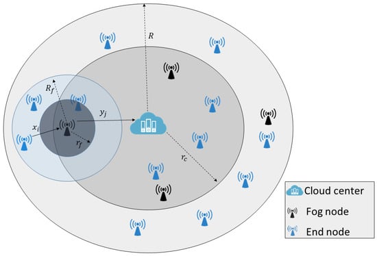
Figure 1. Illustration of the F-RAN model.

We also assumed that all nodes inherently have capabilities of being a FN and can be activated as a FN with a probability p, or deactivated and downgraded to be an EN with probability $1-p$. Consequently, the number of FNs is $n_1=np$ and the number of ENs is $n_0=n(1-p)$. Since the number of FNs is determined by p, it is clear that our problem of optimizing the number of FNs is equivalent to optimizing p, which minimizes the transmission delay.

Note that optimizing the transmission delay w.r.t. the distance automatically optimizes the propagation delay, thus it is omitted. Moreover, as the uplink IoT data are generally transmitted in short data packets, the processing delay of the packet overhead is very small compared with the transmission delay. Also, the FNs can be provided with extra processing capabilities to handle the data traffic at the peak hour, thus the processing delay is assumed to be ignorable.

2.2. Propagation Model

This paper considers both small-scale and large-scale fading. For small-scale fading, a Rayleigh fading channel is assumed, i.e., the small-scale channel gain h follows an exponential distribution with unit mean $h\stackrel{d}{\sim }exp\left(1\right)$. Whereas, the large-scale fading is assumed to be characterized by the inverse power-law path loss models. In the inverse power-law path loss models, the impacts of the environment (outdoor, indoor, rural, urban, suburban, etc.) on the path loss is reflected by the value of the PLE [36,37,38,39]. The path loss models of interest are defined as follows.

Definition 1

(SS-PLM). The standard SS-PLM is given by

$${\ell }_1\left(x\right)=x^{-{\alpha }_x}$$

(1)

where $(x>0)$ denotes the length of the wireless link in meters, and ${\alpha }_x$ stands for the PLE of the link x, which is commonly approximated by a constant in the range of 2 to 5, depending on the propagation environment and the carrier frequency [31].

The limitations of the SS-PLM lead to the consideration of the DS-PLM because it better reflects the PLE dependence on the physical environment in clustered networks and millimetre wave networks.

Definition 2

(DS-PLM). The DS-PLM is defined by [31,34] as;

$${\ell }_2\left(x\right)=\left\{\begin{array}{cc}{x}^{-{\alpha }_{x\left(0\right)}}\hfill & ,x\le r\hfill \\ \eta x^{-{\alpha }_{x\left(1\right)}}\hfill & ,x>r\hfill \end{array}\right.$$

(2)

where $(r>0)$ stands for the critical distance, also known as the break-point distance because the PLE (i.e., slope) changes at it, ${\alpha }_{x\left(0\right)}$ and ${\alpha }_{x\left(1\right)}$ such that $0\le {\alpha }_{x\left(0\right)}\le {\alpha }_{x\left(1\right)}$ are the PLEs of the near- and far-fields, respectively, and $\eta \stackrel{▵}{=}{r}^{\left({\alpha }_{x\left(1\right)}-{\alpha }_{x\left(0\right)}\right)}$ is a factor to maintain the continuity of the path loss.

It should be noted that the critical distance is dependent on the antenna height and the environment, such that it increases with the increase in the antenna height and decreases with the high blocking environment. Generally, it is approximated as the average line-of-sight (LoS) distance of the communication link, whereas the near-field PLE is used to approximate the LoS link regime, and the non-line-of-sight (NLoS) link regime beyond the critical distance is approximated by the far-field PLE [32]. The DS-PLM can be extended to NS-PLM as follows.

Definition 3

(NS-PLM). The NS-PLM is given by [31]

$${\ell }_N({\left\{{\alpha }_{x\left(m\right)}\right\}}_{m=0}^{N-1};x)={\eta }_{\left(m\right)}{x}^{-{\alpha }_{x\left(m\right)}}$$

(3)

for $x\in [r_{(m-1)},r_{\left(m\right)})$, where the 0-th continuity factor is ${\eta }_{\left(0\right)}=1$, the m-th continuity factor can be calculated as ${\eta }_{\left(m\right)}={\prod }_{i=1}^m{r_{\left(m\right)}}^{{\alpha }_{x\left(m\right)}-{\alpha }_{x(m-1)}}$, ${\alpha }_{x\left(m\right)}$ is the m-th PLE such that $0\le {\alpha }_{x\left(0\right)}\le {\alpha }_{x\left(1\right)}\le \cdots \le {\alpha }_{x(N-1)}$, and $r_{\left(m\right)}$ stands for the m-th critical distance such that $0\le r_{\left(0\right)}\le r_{\left(1\right)}\le \cdots \le r_{(N-2)}$.

In the rest of the paper, the notations $r_c$ and $r_f$ are used to denote the critical distances of the cloud and the FN, respectively.

3. Problem Formulation

In the considered system model depicted in Figure 1, we assume that the ENs’ transmitted data in the uplink phase is partially processed at the FN and a portion of it (i.e., non-latency sensitive ones) is relayed to the cloud data center. In other words, if a packet of S bits is delivered via the wireless link to the FN, the FN will process D bits of it, whereas the other $S-D$ bits are forwarded via a wireless link to the cloud data center to perform the necessary processing and computation there. The transmission delay $\tau$ of the considered system model can be calculated as

$$\tau =\frac{S}{{\mathcal{R}}_{fog}}+\frac{S-D}{{\mathcal{R}}_{cloud}}$$

(4)

where the data rate at the FN ${\mathcal{R}}_{fog}$ is given by

$${\mathcal{R}}_{fog}=\mathcal{W}{log}_2\left(1+{\gamma }_{fog}\right)$$

(5)

and the data rate at the cloud ${\mathcal{R}}_{cloud}$ is expressed as

$${\mathcal{R}}_{cloud}=\mathcal{W}{log}_2\left(1+{\gamma }_{cloud}\right)$$

(6)

where $\mathcal{W}$ denotes the link bandwidth. Note that we assumed all the links to have the same bandwidth, and ${\gamma }_{fog}$ and ${\gamma }_{cloud}$ denote SINR of the uplinks at the FN and the cloud, respectively. The SINR of the uplink connecting the i-th EN (i.e., $i=1,2,\cdots ,n_0$) and it’s associated FN (i.e., the j-th FN; $j=1,2,\cdots ,n_1$) is calculated as

$${\gamma }_{fog}^{\left(i\right)}=\frac{P_i{h}_i\ell \left(x_i\right)}{{\sigma }^2+I_{fog}}$$

(7)

where $P_i$ stands for the transmit power of the i-th EN, $h_i$ is the channel gain of the link between the i-th EN and the j-th FN, $x_i$ is the separation distance between the i-th EN and the j-th FN, $\ell \left(x_i\right)$ represents the path loss at a separation distance of $x_i$, ${\sigma }^2$ is the noise power, and $I_{fog}$ is the aggregated interference at the FN, which is originated by the simultaneous transmissions of the other ENs.

The SINR of the uplink from the j-th FN to the cloud data center is given by

$${\gamma }_{cloud}^{\left(j\right)}=\frac{P_j{h}_j\ell \left(y_j\right)}{{\sigma }^2+I_{cloud}}$$

(8)

where $P_j$ denotes the transmit power of the j-th FN, $h_j$ is the channel gain of the link between the j-th FN and the cloud, $y_j$ is the separation distance between the j-th FN and the cloud, $\ell \left(y_j\right)$ is the path loss at a separation distance of $y_j$, and $I_{cloud}$ denotes the aggregated interference at the cloud due to the simultaneous transmissions of the FNs.

For the sake of simplicity, we assumed that the system is noise limited (i.e., $I_{fog}=I_{cloud}=0$) owing to the interference might be perfectly mitigated or because of the pseudo-wired abstraction if wireless links are millimeter waves [40,41].

As stated earlier, our goal is to minimize the transmission delay $\tau$ of the system, hence, the objective function for a single EN (i.e., the i-th EN) transmitting packets through the j-th FN to the cloud can be formulated as

$${\mathcal{J}}_{ij}=min\left(\frac{S}{\mathcal{W}{log}_2\left(1+{\gamma }_{fog}^{\left(i\right)}\right)}+\frac{S-D}{\mathcal{W}{log}_2\left(1+{\gamma }_{cloud}^{\left(j\right)}\right)}\right)$$

(9)

Since $\mathcal{W}$, S, and $S-D$ have constant values they can be omitted as they do not impress the optimization. Consequently, the objective function can be written as

$${\mathcal{J}}_{ij}=min\left(\frac{1}{{log}_2\left(1+{\gamma }_{fog}^{\left(i\right)}\right)}+\frac{1}{{log}_2\left(1+{\gamma }_{cloud}^{\left(j\right)}\right)}\right)$$

(10)

In view of the fact that the logarithm is a monotonic function, the objective function can be rewritten as

$${\mathcal{J}}_{ij}=min\left(\frac{{\sigma }^2}{P_i{h}_i\ell \left(x_i\right)}+\frac{{\sigma }^2}{P_j{h}_j\ell \left(y_j\right)}\right)$$

(11)

Taking the expectation, (11) becomes

$${\widehat{\mathcal{J}}}_{ij}=min\left(\frac{{\sigma }^2}{P_i}E\left[\frac{1}{h_i\ell \left(x_i\right)}\right]+\frac{{\sigma }^2}{P_j}E\left[\frac{1}{h_j\ell \left(y_j\right)}\right]\right)$$

(12)

Here $P_i$ and $P_j$ do not affect the optimization, provided that the receiver has prior knowledge about their values. Also, ${\sigma }^2$ does not influence the optimization process since it can be estimated by the receiver. Moreover, since the channel gains represent the small-scale fading, which is independent of the path loss, the terms containing them can be rewritten as $E\left[1/h_i\ell \left(x_i\right)\right]=E\left[1/h_i\right]E\left[1/\ell \left(x_i\right)\right]$ and $E\left[1/h_j\ell \left(y_j\right)\right]=E\left[1/h_j\right]E\left[1/\ell \left(y_j\right)\right]$, noting that $E\left[1/h_i\right]=E\left[1/h_j\right]$ and equals to a constant value. Thus, they have no impact on the optimization. Therefore, (12) reduces to

$${\widehat{\mathcal{J}}}_{ij}=min\left(E\left[\frac{1}{\ell \left(x_i\right)}\right]+E\left[\frac{1}{\ell \left(y_j\right)}\right]\right)$$

(13)

In the light of the fact that there are $n_0$ ENs and $n_1$ FNs, generalizing (13) for $n_0$ ENs and $n_1$ FN leads to

$$\mathcal{J}=min\left(\sum _{i=1}^{n_0}E\left[\frac{1}{\ell \left(x_i\right)}\right]+\sum _{j=1}^{n_1}E\left[\frac{1}{\ell \left(y_j\right)}\right]\right)$$

(14)

Equation (14) shows that the objective function of the system depends on the reciprocal of the expected value of the path loss for the individual links, which are influenced by the PLEs and the spatial distribution of the nodes. In the following section, we present the mathematical approach of optimizing the number of FNs for the path loss models considered in Section 2.2.

4. The Framework for Optimizing the Number of FNs

In this section, we use the stochastic geometry tool to evaluate the optimum number of FNs in a finite F-RAN. Considering that the number of FN is determined by p, the problem is transformed into optimizing p. Then, (14) can be rewritten as

$$\mathcal{J}=\underset{p}{min}\left(\sum _{i=1}^{n_0}E\left[\frac{1}{\ell \left(x_i\right)}\right]+\sum _{j=1}^{n_1}E\left[\frac{1}{\ell \left(y_j\right)}\right]\right)$$

(15)

Since there are $n_1$ FNs, ${\sum }_{i=1}^{n_0}E\left[1/\ell \left(x_i\right)\right]$ can be reformulated as

$$\sum _{i=1}^{n_0}E\left[\frac{1}{\ell \left(x_i\right)}\right]=n_1\sum _{i=1}^{{\tilde{n}}_0}E\left[\frac{1}{\ell \left(x_i\right)}\right]$$

(16)

where ${\tilde{n}}_0$ denotes the average number of ENs that are associated with a single FN, and it is given by

$${\tilde{n}}_0=\frac{n_0}{n_1}=\frac{1-p}{p}$$

(17)

Accordingly, we assumed that the FNs are located at the centers of identical 2-dimensional balls ${\chi }_j$ (i.e., $b({\chi }_j,R_f);j=1,2,\cdots ,n_1$) that are scattered to cover the entire deployment area, such that each ball contains on average ${\tilde{n}}_0$ ENs. Thus, the radius of the area controlled by a single FN $R_f$ can be obtained by

$${\lambda }_{n_0}{A}_{R_f}=\frac{n_0}{n_1}$$

(18)

where ${\lambda }_{n_0}=n_0/\pi R^2$ is the EN density, and $A_{R_f}=\pi R_f^2$ is the area of $b({\chi }_j,R_f)$, hence, we have

$$R_f=\frac{R}{\sqrt{n_1}}=\frac{R}{\sqrt{np}}$$

(19)

In the following subsections, we derive the objective function regarding optimizing the number of FNs for SS-PLM, DS-PLM, and NS-PLM.

4.1. Single-Slope

The objective function utilizing SS-PLM can be written as

$$\begin{array}{cc}\hfill {\mathcal{J}}_1& =\underset{p}{min}\left(n_1\sum _{i=1}^{{\tilde{n}}_0}E\left[\frac{1}{{\ell }_1\left(x_i\right)}\right]+\sum _{j=1}^{n_1}E\left[\frac{1}{{\ell }_1\left(y_j\right)}\right]\right)\hfill \\ \hfill & =\underset{p}{min}\left(n_1\sum _{i=1}^{{\tilde{n}}_0}E\left[\frac{1}{x_i^{-{\alpha }_x}}\right]+\sum _{j=1}^{n_1}E\left[\frac{1}{y_j^{-{\alpha }_y}}\right]\right)\hfill \\ \hfill & =\underset{p}{min}\left(n_1\sum _{i=1}^{{\tilde{n}}_0}E\left[x_i^{{\alpha }_x}\right]+\sum _{j=1}^{n_1}E\left[y_j^{{\alpha }_y}\right]\right)\hfill \end{array}$$

(20)

According to [18], the ${\alpha }_x$-th moment of the distance between the center of the 2-dimensional ball $b({\chi }_j,R_f)$ that encloses ${\tilde{n}}_0$ nodes and the i-th nearest BPP node is given by

$$E\left[x_i^{{\alpha }_x}\right]=\frac{R_f^{{\alpha }_x}{i}^{\left[{\alpha }_x/2\right]}}{{\left({\tilde{n}}_0+1\right)}^{\left[{\alpha }_x/2\right]}}$$

(21)

where ${\zeta }^{\left[\kappa \right]}=\mathsf{\Gamma }(\zeta +\kappa )/\mathsf{\Gamma }\left(\zeta \right)$ is the Pochhammer function notation (sometimes called the raising factorial), and $\mathsf{\Gamma }\left(\zeta \right)=(\zeta -1)!$ denotes the gamma function.

Generalizing (21) for ${\tilde{n}}_0$ ENs, this yields

$$\sum _{i=1}^{{\tilde{n}}_0}E\left[x_i^{{\alpha }_x}\right]=\frac{R_f^{{\alpha }_x}}{{\left({\tilde{n}}_0+1\right)}^{\left[{\alpha }_x/2\right]}}\sum _{i=1}^{{\tilde{n}}_0}{i}^{\left[{\alpha }_x/2\right]}$$

(22)

Using mathematical induction, we have

$$\sum _{i=1}^{{\tilde{n}}_0}{i}^{\left[{\alpha }_x/2\right]}=\frac{{\tilde{n}}_0}{1+{\alpha }_x/2}{\left({\tilde{n}}_0+1\right)}^{\left[{\alpha }_x/2\right]}$$

(23)

Substituting (23) into (22), the following closed-form is obtained

$$\sum _{i=1}^{{\tilde{n}}_0}E\left[x_i^{{\alpha }_x}\right]=\frac{R_f^{{\alpha }_x}{\tilde{n}}_0}{1+{\alpha }_x/2}$$

(24)

Analogously, since the FNs are scattered according to BPP in $b\left(\mathit{o},R\right)$, we have

$$\sum _{j=1}^{n_1}E\left[y_j^{{\alpha }_y}\right]=\frac{R^{{\alpha }_y}{n}_1}{1+{\alpha }_y/2}$$

(25)

Therefore, the objective function utilizing SS-PLM can be expressed as

$$\begin{array}{cc}\hfill {\mathcal{J}}_1& =\underset{p}{min}\left(\frac{n_0{R}_f^{{\alpha }_x}}{1+{\alpha }_x/2}+\frac{n_1{R}^{{\alpha }_y}}{1+{\alpha }_y/2}\right)\hfill \\ \hfill & =\underset{p}{min}\left(\frac{n(1-p){\left(\frac{R}{\sqrt{np}}\right)}^{{\alpha }_x}}{1+{\alpha }_x/2}+\frac{np{R}^{{\alpha }_y}}{1+{\alpha }_y/2}\right)\hfill \end{array}$$

(26)

Lemma 1.

The objective function utilizing SS-PLM in (26) is strictly convex, and hence there is a unique global value of p that minimizes it.

Proof. 

The convexity of the objective function can be proven by the second derivative test. The second derivative of ${\mathcal{J}}_1$ w.r.t p is;

$$\frac{{\partial }^2{\mathcal{J}}_1}{\partial p^2}=\frac{n{\alpha }_x{\left(\frac{R}{\sqrt{np}}\right)}^{{\alpha }_x}}{2+{\alpha }_x}\left(\frac{2+(1-p)(({\alpha }_x/2)-1)}{p^2}\right)$$

(27)

one can observe that the second derivative is positive for $0<p<1$. Therefore, ${\mathcal{J}}_1$ is strictly convex and hence there is a unique optimum value of p that minimizes it. □

The global value of p that minimizes ${\mathcal{J}}_1$ can be obtained by solving for the real root in the range $0<p<1$ of

$$\frac{\partial {\mathcal{J}}_1}{\partial p}=0$$

(28)

which can be rewritten after performing some operations as the following polynomial equation of the degree $\left(1+{\alpha }_x/2\right)$

$$p^{\left(1+{\alpha }_x/2\right)}+c_{1}p+c_0=0$$

(29)

where

$$c_0=\frac{-{\alpha }_x\left(1+{\alpha }_y/2\right)R^{{\alpha }_x-{\alpha }_y}}{2\left(1+{\alpha }_x/2\right)n^{{\alpha }_x/2}}$$

(30)

and

$$c_1=\frac{\left({\alpha }_x-2\right)\left(1+{\alpha }_y/2\right)R^{{\alpha }_x-{\alpha }_y}}{2\left(1+{\alpha }_x/2\right)n^{{\alpha }_x/2}}$$

(31)

The optimum value of p and $n_1$ for the special cases of ${\alpha }_x=2$ and ${\alpha }_x=4$ are presented in Corollaries 1 and 2, respectively.

Corollary 1.

The optimum value of p and $n_1$ utilizing SS-PLM at ${\alpha }_{x\left(1\right)}=2$ are

$$p=\sqrt{-c_0}$$

(32)

and

$$n_1=n\sqrt{-c_0}$$

(33)

respectively.

Proof. 

When ${\alpha }_x=2$, Equation (29) becomes a quadratic equation, and $c_1=0$. Hence, the optimum value of p is computed as the square root of the constant $-c_0$.  □

Corollary 2.

When ${\alpha }_x=4$, the closed-form expression of the optimum value of p and $n_1$ utilizing SS-PLM can be calculated by

$$p=-\frac{1}{3}\left(u_2+\frac{u_0}{u_2}\right)$$

(34)

and

$$n_1=-\frac{n}{3}\left(u_2+\frac{u_0}{u_2}\right)$$

(35)

respectively, where

$$u_0=-3c_1$$

(36)

$$u_1=27c_0$$

(37)

and

$$u_2=\sqrt[3]{\frac{u_1+\sqrt{u_1^2-4u_0^3}}{2}}$$

(38)

Proof. 

Equation (29) is a cubic equation when ${\alpha }_x=4$. Therefore, the optimum value of p is the cubic equation’s root given in (34).  □

4.2. Dual-Slope

When DS-PLM is utilized, the objective function can be expressed as

$${\mathcal{J}}_2=\underset{p}{min}\left(n_1\sum _{i=1}^{{\tilde{n}}_0}E\left[\frac{1}{{\ell }_2\left(x_i\right)}\right]+\sum _{j=1}^{n_1}E\left[\frac{1}{{\ell }_2\left(y_j\right)}\right]\right)$$

(39)

Bearing in mind that DS-PLM has different PLEs for the range of distances less than and higher than the critical radius of the FN $r_f$. Therefore, ${\sum }_{i=1}^{{\tilde{n}}_0}E\left[1/{\ell }_2\left(x_i\right)\right]$ can be expressed as

$$\begin{array}{cc}\hfill \sum _{i=1}^{{\tilde{n}}_0}E\left[\frac{1}{{\ell }_2\left(x_i\right)}\right]& =\sum _{i=1}^{{\tilde{n}}_{0\left(0\right)}}E\left[\frac{1}{x_i^{-{\alpha }_{x\left(0\right)}}}\right]+\sum _{i={\tilde{n}}_{0\left(0\right)}+1}^{{\tilde{n}}_0}E\left[\frac{1}{\eta x_i^{-{\alpha }_{x\left(1\right)}}}\right]\hfill \\ \hfill & =\sum _{i=1}^{{\tilde{n}}_{0\left(0\right)}}E\left[x_i^{{\alpha }_{x\left(0\right)}}\right]+r_f^{{\alpha }_{x\left(0\right)}-{\alpha }_{x^{\left(1\right)}}}\sum _{i={\tilde{n}}_{0\left(0\right)}+1}^{{\tilde{n}}_0}E\left[x_i^{{\alpha }_{x\left(1\right)}}\right]\hfill \end{array}$$

(40)

where ${\tilde{n}}_{0\left(0\right)}$ is the expected number of ENs that reside inside $r_f$.

$${\tilde{n}}_{0\left(0\right)}={\lambda }_{n_0}{A}_{r_f}=n(1-p){\left(\frac{r_f}{R}\right)}^2$$

(41)

where $A_{r_f}=\pi r_f^2$ is the area enclosed by $b({\chi }_j,r_f)$. Since ${\tilde{n}}_{0\left(0\right)}$ ENs are scattered according to BPP within $b({\chi }_j,r_f)$, identity (24) can be used to obtain the following closed-form expression

$$\sum _{i=1}^{{\tilde{n}}_{0\left(0\right)}}E\left[x_i^{{\alpha }_{x\left(0\right)}}\right]=\frac{r_f^{{\alpha }_{x\left(0\right)}}{\tilde{n}}_{0\left(0\right)}}{1+{\alpha }_{x\left(0\right)}/2}$$

(42)

whereas the ${\alpha }_{x\left(1\right)}$-th moment of the distance from the center of the ball $b({\chi }_j,R_f)$ to the i-th node that is located beyond $r_f$ can be obtained by

$$E\left[x_i^{{\alpha }_{x\left(1\right)}}\right]={\int }_{r_f}^{R_f}{x}^{{\alpha }_{x\left(1\right)}}{f}_{X_i}\left(x\right|X_{{\tilde{n}}_{0\left(0\right)}}=r_f)dx$$

(43)

where the distance distribution function is given by [18]

$$f_{X_i}\left(x\right|X_{{\tilde{n}}_{0\left(0\right)}}=r_f)=\frac{2x}{R_f^2-r_f^2}\frac{{(1-q)}^{{\tilde{n}}_0-i}{q}^{i-{\tilde{n}}_{0\left(0\right)}-1}}{\beta ({\tilde{n}}_0-i+1,i-{\tilde{n}}_{0\left(0\right)})}$$

(44)

where $\beta (a,b)=\mathsf{\Gamma }\left(a\right)\mathsf{\Gamma }\left(b\right)/\mathsf{\Gamma }(a+b)$ is the beta function, and $q=(x^2-r_f^2)/(R_f^2-r_f^2)$.

Then, we have

$$\begin{array}{cc}\hfill E\left[x_i^{{\alpha }_{x\left(1\right)}}\right]& ={\int }_{r_f}^{R_f}\frac{2x^{{\alpha }_{x\left(1\right)}+1}}{R_f^2-r_f^2}\frac{{(1-q)}^{{\tilde{n}}_0-i}{q}^{i-{\tilde{n}}_{0\left(0\right)}-1}}{\beta ({\tilde{n}}_0-i+1,i-{\tilde{n}}_{0\left(0\right)})}dx\hfill \\ \hfill & =\frac{r_f^{{\alpha }_{x\left(1\right)}}}{\beta ({\tilde{n}}_0-i+1,i-{\tilde{n}}_{0\left(0\right)})}{\int }_0^1{q}^{i-{\tilde{n}}_{0\left(0\right)}-1}{(1-q)}^{{\tilde{n}}_0-i}{\left(1-\left(1-{\left(\frac{R_f}{r_f}\right)}^2\right)q\right)}^{{\alpha }_{x\left(1\right)}/2}dq\hfill \\ \hfill & =r_f^{{\alpha }_{x\left(1\right)}}{}_2{\mathrm{F}}_1\left(\begin{array}{ccc}-{\alpha }_{x\left(1\right)}/2& & i-{\tilde{n}}_{0\left(0\right)}\\ & {\tilde{n}}_0-{\tilde{n}}_{0\left(0\right)}+1\end{array};1-{\left(\frac{R_f}{r_f}\right)}^2\right)\hfill \end{array}$$

(45)

where ${}_2{\mathrm{F}}_1\left(\begin{array}{ccc}a& & b\\ & c\end{array};z\right)$ stands for Gauss hypergeometric function.

Generalizing (45) for (${\tilde{n}}_0-{\tilde{n}}_{0\left(0\right)}$) ENs, then using the series representation of ${}_2{\mathrm{F}}_1$ yields:

$$\begin{array}{cc}\hfill \sum _{i={\tilde{n}}_{0\left(0\right)}+1}^{{\tilde{n}}_0}E\left[x_i^{{\alpha }_{x\left(1\right)}}\right]& =\sum _{i={\tilde{n}}_{0\left(0\right)}+1}^{{\tilde{n}}_0}{r}_f^{{\alpha }_{x\left(1\right)}}{}_2{\mathrm{F}}_1\left(\begin{array}{ccc}-{\alpha }_{x\left(1\right)}/2& & i-{\tilde{n}}_{0\left(0\right)}\\ & {\tilde{n}}_0-{\tilde{n}}_{0\left(0\right)}+1\end{array};1-{\left(\frac{R_f}{r_f}\right)}^2\right)\hfill \\ \hfill & =\sum _{i={\tilde{n}}_{0\left(0\right)}+1}^{{\tilde{n}}_0}{r}_f^{{\alpha }_{x\left(1\right)}}\sum _{k=0}^{\infty }\frac{{(-{\alpha }_{x\left(1\right)}/2)}^{\left[k\right]}{(i-{\tilde{n}}_{0\left(0\right)})}^{\left[k\right]}}{{({\tilde{n}}_0-{\tilde{n}}_{0\left(0\right)}+1)}^{\left[k\right]}}\frac{{\left(1-{\left(\frac{R_f}{r_f}\right)}^2\right)}^k}{k!}\hfill \\ \hfill & =r_f^{{\alpha }_{x\left(1\right)}}\sum _{k=0}^{\infty }\frac{{(-{\alpha }_{x\left(1\right)}/2)}^{\left[k\right]}{\sum }_{i=1}^{{\tilde{n}}_0-{\tilde{n}}_{0\left(0\right)}}{i}^{\left[k\right]}}{{({\tilde{n}}_0-{\tilde{n}}_{0\left(0\right)}+1)}^{\left[k\right]}}\frac{{\left(1-{\left(\frac{R_f}{r_f}\right)}^2\right)}^k}{k!}\hfill \end{array}$$

(46)

Using identity (23), we have

$$\begin{array}{cc}\hfill \sum _{i={\tilde{n}}_{0\left(0\right)}+1}^{{\tilde{n}}_0}E\left[x_i^{{\alpha }_{x\left(1\right)}}\right]& =r_f^{{\alpha }_{x\left(1\right)}}({\tilde{n}}_0-{\tilde{n}}_{0\left(0\right)})\sum _{k=0}^{\infty }\frac{{(-{\alpha }_{x\left(1\right)}/2)}^{\left[k\right]}}{k+1}\frac{{\left(1-{\left(\frac{R_f}{r_f}\right)}^2\right)}^k}{k!}\hfill \\ \hfill & =r_f^{{\alpha }_{x\left(1\right)}}({\tilde{n}}_0-{\tilde{n}}_{0\left(0\right)})\sum _{k=0}^{\infty }\frac{\mathsf{\Gamma }(k+1){(-{\alpha }_{x\left(1\right)}/2)}^{\left[k\right]}}{\mathsf{\Gamma }(k+2)}\frac{{\left(1-{\left(\frac{R_f}{r_f}\right)}^2\right)}^k}{k!}\hfill \\ \hfill & =r_f^{{\alpha }_{x\left(1\right)}}({\tilde{n}}_0-{\tilde{n}}_{0\left(0\right)}){}_2{\mathrm{F}}_1\left(\begin{array}{ccc}-{\alpha }_{x\left(1\right)}/2& & 1\\ & 2\end{array};1-{\left(\frac{R_f}{r_f}\right)}^2\right)\hfill \end{array}$$

(47)

It can be verified that,

$${}_2{\mathrm{F}}_1\left(\begin{array}{ccc}-{\alpha }_{x\left(1\right)}/2& & 1\\ & 2\end{array};1-{\left(\frac{R_f}{r_f}\right)}^2\right)=\frac{\left(1-{\left(\frac{R_f}{r_f}\right)}^{\left(2+{\alpha }_{x\left(1\right)}\right)}\right)}{\left(1-{\left(\frac{R_f}{r_f}\right)}^2\right)\left(1+{\alpha }_{x\left(1\right)}/2\right)}$$

(48)

Then, we obtain

$$\sum _{i={\tilde{n}}_{0\left(0\right)}+1}^{{\tilde{n}}_0}E\left(x_i^{{\alpha }_{x\left(1\right)}}\right)=\frac{r_f^{{\alpha }_{x\left(1\right)}}({\tilde{n}}_0-{\tilde{n}}_{0\left(0\right)})\left(1-{\left(\frac{R_f}{r_f}\right)}^{\left(2+{\alpha }_{x\left(1\right)}\right)}\right)}{\left(1-{\left(\frac{R_f}{r_f}\right)}^2\right)\left(1+{\alpha }_{x\left(1\right)}/2\right)}$$

(49)

therefore, the closed-form expression of ${\sum }_{i=1}^{{\tilde{n}}_0}E\left[1/{\ell }_2\left(x_i\right)\right]$ can be expressed as

$$\sum _{i=1}^{{\tilde{n}}_0}E\left[\frac{1}{{\ell }_2\left(x_i\right)}\right]=r_f^{{\alpha }_{x\left(0\right)}}\left(\frac{{\tilde{n}}_{0\left(0\right)}}{1+{\alpha }_{x\left(0\right)}/2}+\frac{({\tilde{n}}_0-{\tilde{n}}_{0\left(0\right)})\left(1-{\left(\frac{R_f}{r_f}\right)}^{\left(2+{\alpha }_{x\left(1\right)}\right)}\right)}{\left(1-{\left(\frac{R_f}{r_f}\right)}^2\right)\left(1+{\alpha }_{x\left(1\right)}/2\right)}\right)$$

(50)

Since there is a single cloud center, following the same steps of deriving (50), the closed-form expression of ${\sum }_{j=1}^{n_1}E\left[1/{\ell }_2\left(y_j\right)\right]$ can be obtained as

$$\sum _{j=1}^{n_1}E\left[\frac{1}{{\ell }_2\left(y_j\right)}\right]=r_c^{{\alpha }_{y\left(0\right)}}\left(\frac{n_{1\left(0\right)}}{1+{\alpha }_{y\left(0\right)}/2}+\frac{(n_1-n_{1\left(0\right)})\left(1-{\left(\frac{R}{r_c}\right)}^{\left(2+{\alpha }_{y\left(1\right)}\right)}\right)}{\left(1-{\left(\frac{R}{r_c}\right)}^2\right)\left(1+{\alpha }_{y\left(1\right)}/2\right)}\right)$$

(51)

where ${\alpha }_{y\left(0\right)}$ and ${\alpha }_{y\left(1\right)}$ are the PLEs before and beyond $r_c$, respectively, and $n_{1\left(0\right)}$ is the expected number of FNs that lay inside $b\left(\mathit{o},r_c\right)$, which can be calculated as

$$n_{1\left(0\right)}={\lambda }_{n_1}{A}_{r_c}=np{\left(\frac{r_c}{R}\right)}^2$$

(52)

where ${\lambda }_{n_1}=n_1/\pi R^2$, which denotes the FN density, and $A_{r_c}=\pi r_c^2$, which stands for the area of $b(\mathit{o},r_c)$.

Then, the objective function that utilizes DS-PLM can be expressed as

$${\mathcal{J}}_2=\underset{p}{min}\left(\begin{array}{c}{n}_1{r}_f^{{\alpha }_{x\left(0\right)}}\left(\frac{{\tilde{n}}_{0\left(0\right)}}{1+{\alpha }_{x\left(0\right)}/2}+\frac{({\tilde{n}}_0-{\tilde{n}}_{0\left(0\right)})\left(1-{\left(\frac{R_f}{r_f}\right)}^{\left(2+{\alpha }_{x\left(1\right)}\right)}\right)}{\left(1-{\left(\frac{R_f}{r_f}\right)}^2\right)\left(1+{\alpha }_{x\left(1\right)}/2\right)}\right)\hfill \\ +r_c^{{\alpha }_{y\left(0\right)}}\left(\frac{n_{1\left(0\right)}}{1+{\alpha }_{y\left(0\right)}/2}+\frac{(n_1-n_{1\left(0\right)})\left(1-{\left(\frac{R}{r_c}\right)}^{\left(2+{\alpha }_{y\left(1\right)}\right)}\right)}{\left(1-{\left(\frac{R}{r_c}\right)}^2\right)\left(1+{\alpha }_{y\left(1\right)}/2\right)}\right)\hfill \end{array}\right)$$

(53)

Substituting the values of $n_1$, $n_{1\left(0\right)}$, ${\tilde{n}}_0$, ${\tilde{n}}_{0\left(0\right)}$, and $R_f$ into (53), we obtain

$${\mathcal{J}}_2=\underset{p}{min}\left(\begin{array}{c}\frac{np(1-p)r_f^{{\alpha }_{x\left(0\right)}}}{Q}\left(\frac{1}{\left(1+{\alpha }_{x\left(0\right)}/2\right)}-\frac{\left(1-{\left(\frac{Q}{p}\right)}^{\left(1+{\alpha }_{x\left(1\right)}/2\right)}\right)}{\left(1+{\alpha }_{x\left(1\right)}/2\right)}\right)\hfill \\ +\frac{np{r}_c^{{\alpha }_{y\left(0\right)}}}{W}\left(\frac{1}{\left(1+{\alpha }_{y\left(0\right)}/2\right)}-\frac{\left(1-W^{\left(1+{\alpha }_{y\left(1\right)}/2\right)}\right)}{\left(1+{\alpha }_{y\left(1\right)}/2\right)}\right)\hfill \end{array}\right)$$

(54)

where $Q=R^2/n{r}_f^2$ and $W=R^2/r_c^2$.

Lemma 2.

There is a unique optimum global value of p in the range $0<p<1$ such that $p<R^2/\left(n{r}_f^2\right)$ (i.e., $R_f>r_f$) that minimizes (54).

Proof. 

To prove that (54) is strictly convex in the range of p as specified in Lemma 2, the second derivative test is used. The second derivative of (54) w.r.t. p is

$$\frac{{\partial }^2{\mathcal{J}}_2}{\partial p^2}=\frac{2n{r}_f^{{\alpha }_{x\left(0\right)}}}{Q}\left(\begin{array}{c}\left(\frac{{\alpha }_{x\left(1\right)}}{2}{\left(\frac{Q}{p}\right)}^{\left(1+{\alpha }_{x\left(1\right)}/2\right)}\left(\frac{\left(1-p\right)}{2p}+\frac{1}{\left(1+{\alpha }_{x\left(1\right)}/2\right)}\right)\right)\hfill \\ -\left(\frac{1}{\left(1+{\alpha }_{x\left(0\right)}/2\right)}-\frac{1}{\left(1+{\alpha }_{x\left(1\right)}/2\right)}\right)\hfill \end{array}\right)$$

(55)

After performing some mathematical operations on (55), we have;

$${\left(\frac{Q}{p}\right)}^{\left(1+{\alpha }_{x\left(1\right)}/2\right)}\left(\frac{\left(1+{\alpha }_{x\left(1\right)}/2\right)\left(1-p\right)}{2p}+1\right)-\left(\frac{1-\left({\alpha }_{x\left(0\right)}/{\alpha }_{x\left(1\right)}\right)}{1+{\alpha }_{x\left(0\right)}/2}\right)>0$$

(56)

It can be observed that inequality in (56) is satisfied since the first term of the left-hand side is always greater than one for any value of p in its specified range, while the second term is less than one. Therefore, (54) is strictly convex in the specified range, and hence there is a unique global optimum value of p, which minimizes (54). □

The global optimum value of p is the real root in the specified range in Lemma 2 of:

$$\frac{\partial {\mathcal{J}}_2}{\partial p}=0$$

(57)

which can be rewritten after some simple algebraic operations as:

$$p^{\left(2+{\alpha }_{x\left(1\right)}/2\right)}+a_2{p}^{\left(1+{\alpha }_{x\left(1\right)}/2\right)}+a_{1}p+a_0=0$$

(58)

where

$$a_0=Q^{\left(1+{\alpha }_{x\left(1\right)}/2\right)}\left(\frac{\left(1+{\alpha }_{x\left(0\right)}/2\right)\left({\alpha }_{x\left(1\right)}/2\right)}{{\alpha }_{x\left(1\right)}-{\alpha }_{x\left(0\right)}}\right)$$

(59)

$$a_1=Q^{\left(1+{\alpha }_{x\left(1\right)}/2\right)}\left(\frac{\left(1+{\alpha }_{x\left(0\right)}/2\right)\left(1-{\alpha }_{x\left(1\right)}/2\right)}{{\alpha }_{x\left(1\right)}-{\alpha }_{x\left(0\right)}}\right)$$

(60)

and

$$a_2=\frac{\left(1+{\alpha }_{x\left(0\right)}/2\right)\left(1+{\alpha }_{x\left(1\right)}/2\right)}{n\left({\alpha }_{x\left(1\right)}-{\alpha }_{x\left(0\right)}\right)}\frac{r_c^{{\alpha }_{y\left(0\right)}+2}}{r_f^{{\alpha }_{x\left(0\right)}+2}}\left(\frac{\left(1-W^{\left(1+{\alpha }_{y\left(1\right)}/2\right)}\right)}{\left(1+{\alpha }_{y\left(1\right)}/2\right)}-\frac{1}{\left(1+{\alpha }_{y\left(0\right)}/2\right)}\right)-\frac{1}{2}$$

(61)

Note that (58) is a polynomial equation of the degree ($2+{\alpha }_{x\left(1\right)}/2$), which can be solved numerically, by factorization, using algebraic geometry, or any other possible method. For example, the well-known Graeffe’s method of solving polynomial equations can be used to compute all the roots of (29) and (58), where the computational complexity estimation indicates that all the roots can be computed using $O({\theta }^{2}log\theta (\theta log\theta +log(1/ϵ)))$ arithmetic operations, where $\theta$ is the degree of the polynomial and $ϵ>0$ is the relative output error bound [42]. In the following corollaries, we provide closed-form expressions of the optimum values of p and $n_1$ for the special cases of the far-field PLEs of the links between the ENs and the FN are ${\alpha }_{x\left(1\right)}=2$ and ${\alpha }_{x\left(1\right)}=4$.

Corollary 3.

When ${\alpha }_{x\left(1\right)}=2$, the closed-form expression of the optimum values of p and $n_1$ can be obtained by

$$p=-\frac{1}{3}\left(a_2+b_2+\frac{b_0}{b_2}\right)$$

(62)

as consequence, the optimum number of FNs is given as

$$n_1=-\frac{n}{3}\left(a_2+b_2+\frac{b_0}{b_2}\right)$$

(63)

where

$$b_0=a_2^2$$

(64)

$$b_1=2a_2^3+27a_0$$

(65)

and

$$b_2=\sqrt[3]{\frac{b_1+\sqrt{b_1^2-4b_0^3}}{2}}$$

(66)

Proof. 

Substituting ${\alpha }_{x\left(1\right)}=2$ into (58), it reduces to a cubic equation. Hence, the optimum value of p is obtained as in (62) by solving for the real root in the specified range of p in Lemma 2.  □

Corollary 4.

When ${\alpha }_{x\left(1\right)}=4$, the optimum value of p can be expressed as

$$p=-\frac{a_2}{4}-g_5+\frac{1}{2}\sqrt{-4g_5^2-2g_0+{\displaystyle \frac{g_1}{g_5}}}$$

(67)

accordingly, the optimum number of FNs can be computed by:

$$n_1=n\left(-\frac{a_2}{4}-g_5+\frac{1}{2}\sqrt{-4g_5^2-2g_0+{\displaystyle \frac{g_1}{g_5}}}\right)$$

(68)

where

$$g_0=\frac{-3a_2^2}{8}$$

(69)

$$g_1=\frac{a_2^3}{8}+a_1$$

(70)

$$g_2=-3a_2{a}_1+12a_0$$

(71)

$$g_3=27\left(a_2^2{a}_0+a_1^2\right)$$

(72)

$$g_4=\sqrt[3]{\frac{g_3+\sqrt{g_3^2-4g_2^3}}{2}}$$

(73)

and

$$g_5=\frac{1}{2}\sqrt{\frac{1}{3}\left(-2g_0+g_4+\frac{g_2}{g_4}\right)}$$

(74)

Proof. 

Equation (58) becomes a quartic equation when ${\alpha }_{x\left(1\right)}=4$. Therefore, the optimum value of p given by (67) is the real root of the quartic equation in the range stated in Lemma 2.  □

4.3. N-Slope

The objective funcyion utilizing DS-PLM can be extended to NS-PLM as in Lemma 3.

Lemma 3.

The objective function that utilizes NS-PLM can be formulated as

$${\mathcal{J}}_{\mathcal{N}}=\underset{p}{min}\left(\begin{array}{c}{n}_1\left(\frac{{\tilde{n}}_{0\left(0\right)}{r}_{f\left(0\right)}^{{\alpha }_{x\left(0\right)}}}{1+{\alpha }_{x\left(0\right)}/2}+\sum _{m=1}^{N-1}{r}_{f\left(m\right)}^{{\alpha }_{x\left(m\right)}}{\eta }_{f\left(m\right)}({\tilde{n}}_{0\left(m\right)}-{\tilde{n}}_{0(m-1)}){}_2{\mathrm{F}}_1\left(\begin{array}{ccc}-{\alpha }_{x\left(m\right)}/2& & 1\\ & 2\end{array};{\nu }_f\right)\right)\hfill \\ +\frac{n_{1\left(0\right)}{r}_{c\left(0\right)}^{{\alpha }_{y\left(0\right)}}}{1+{\alpha }_{y\left(0\right)}/2}+\sum _{m=1}^{N-1}{r}_{c\left(m\right)}^{{\alpha }_{y\left(m\right)}}{\eta }_{c\left(m\right)}(n_{1\left(m\right)}-n_{1(m-1)}){}_2{\mathrm{F}}_1\left(\begin{array}{ccc}-{\alpha }_{y\left(m\right)}/2& & 1\\ & 2\end{array};{\nu }_c\right)\hfill \end{array}\right)$$

(75)

where $r_{f\left(m\right)}$ and $r_{c\left(m\right)}$; $m=0,1,..N-2$ are the $m-th$ critical distance of the FN and the cloud, respectively. Furthermore, $r_{f(N-1)}=R/\sqrt{n_1}$ and $r_{c(N-1)}=R$ are the maximum radius of the FN and the cloud, respectively. The parameters ${\eta }_{f\left(m\right)}$ and ${\eta }_{c\left(m\right)}$ are the fog and cloud path loss model continuity factors. Whereas ${\tilde{n}}_{0\left(m\right)}$ denotes the expected number of ENs inside $b({\chi }_j,r_{f\left(m\right)})$ such that ${\tilde{n}}_{0(N-1)}=n_0/n_1$, and $n_{1\left(m\right)}$ is the expected number of FNs that reside in $b(\mathit{o},r_{c\left(m\right)})$ where $n_{1(N-1)}=n_1$, ${\nu }_f=1-{\left(r_{f\left(m\right)}/r_{f(m-1)}\right)}^2$ and ${\nu }_c=1-{\left(r_{c\left(m\right)}/r_{c(m-1)}\right)}^2$.

Proof. 

The objective function utilizing NS-PLM can be derived by following the same steps of deriving ${\mathcal{J}}_2$, where $E\left[x_i^{{\alpha }_{x\left(m\right)}}\right]$ can be obtained by setting the integral limits in (54) from $r_{f(m-1)}$ to $r_{f\left(m\right)}$.  □

The optimum number of FNs for NS-PLM can be calculated by solving for the real root of the first derivative of the objective function or using any numerical method when the closed-form of the root cannot be obtained due to the complexity.

5. Numerical Results

Here, we present the numerical results of optimizing the number of FNs in a finite BPP F-RAN. We studied the impacts of the DS-PLM parameters on the optimum number of FNs, including the PLEs of near- and far-fields, and the critical distance. Also, the impact of the number of nodes scattered in the deployment area is analysed.

We consider a disk-shaped deployment area of a radius $R=5$ km, in which the cloud data center is located at the center, and the nodes are uniformly scattered according to BPP. In order to analyse the impacts of the network parameters on the optimum number of FNs, we plot the objective function in (54) w.r.t. p for various values of the considered parameter. Moreover, Matlab simulations were performed, in which a noise spectral density of $-174$ dBm/Hz and a bandwidth of $\mathcal{W}=1$ GHz are assumed, to study the average transmission delay of an EN that transmits a packet size of $S=1$ kbit to the FN, which in turn forwards $50\%$ of it to the cloud. The average delay for a single EN is obtained by averaging after performing 1 million iterations for both optimized and unoptimized number of FNs cases. In the optimized case, we fixed the number of FNs to be equal to the optimum number in all the iterations. Whereas in the unoptimized case, a random number of FNs (such that $0<n_1<n$) is generated for each iteration. Note that the y axis in all figures in this section is in log scale.

In Figure 2, we illustrate the objective function that utilizes SS-PLM for ${\alpha }_x={\alpha }_y=4$. The figure reveals that our optimization approach, which assumes that the FNs are scattered to cover the deployment area, achieves lower optimum probabilities of being a FN, and hence a few FNs are required to optimize the performance compared with the approach presented in [24], which assumes that the FNs constitute a circular mesh around the cloud data center.

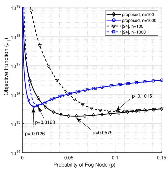
Figure 2. The objective function vs. p utilizing SS-PLM at ${\alpha }_x={\alpha }_y=4$.

The relationship between the PLEs of the uplink from the EN to the FN and the objective function is illustrated in Figure 3. Wherein we plot the objective function versus p for various combinations of the near- and far-field PLEs of the wireless uplink from the EN to the FN. It can be observed that the objective function curves have a unique minimum point, which represents the optimum value of the probability of being a FN, which in turn specifies the optimum number of FNs. The values of the optimum p, $n_1$, and the average number of ENs per each FN that corresponds to Figure 3 are given in Table 1. The results show that when the links from the ENs to the FNs experience low PLEs (i.e., ${\alpha }_{x\left(0\right)}=2$ and ${\alpha }_{x\left(1\right)}=3$), a small percentage of the nodes, which is 3.39% (i.e., about 17 nodes), needs to be upgraded to FNs to optimize the transmission delay in the considered F-RAN. In this case, it is noteworthy to highlight that the increase in the number of FNs will not improve the performance because more FNs will be located at the edge of the network, and thus the direct links between them and the cloud will experience higher path losses due to the larger distance to the cloud compared with the distance to the closest FN, which in turn degrade the performance. In the second case, when the far-field PLE of the links from the ENs to the cloud increases (i.e., ${\alpha }_{x\left(1\right)}=4$), the farthest nodes from the FNs will experience higher path losses, hence a larger number of FNs compared with the first case is required to improve the performance, which is about 34 FNs. However, as the links to the FNs experience severe path losses due to the higher PLE of the near-field (i.e., ${\alpha }_{x\left(0\right)}=3$), the value of p that optimizes the transmission delay leaps to 0.2169 (i.e., about 108 FNs) with about 3.61 ENs on average being associated with each FN. Hence, in the non-latency sensitive IoT systems, the direct communication between the ENs and the cloud might be more efficient and cost-saving due to the cost of the large number of FNs that need extra computational capabilities. Hence, a trade-off between the delay and the cost should be done in this case. Moreover, it is noteworthy to point out that as links to the FNs experience lower path losses, additional computational capabilities should be provided to the FNs since a larger number of ENs will be associated with each FN.

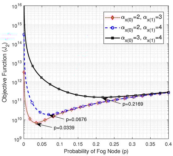
Figure 3. The objective function vs. p at $n=500$, ${\alpha }_{y\left(0\right)}=2$, ${\alpha }_{y\left(1\right)}=3$, $r_f=100m$, and $r_c=500m$.

Table 1. The optimum value of p, $n_1$, and $n_0/n_1$ at $n=500$, ${\alpha }_{y\left(0\right)}=2$, ${\alpha }_{y\left(1\right)}=3$, $r_f=100m$, and $r_c=500m$.

${\mathit{\alpha }}_{\mathit{x}\mathbf{\left(}\mathbf{0}\mathbf{\right)}}$	${\mathit{\alpha }}_{\mathit{x}\mathbf{\left(}\mathbf{1}\mathbf{\right)}}$	p	${\mathit{n}}_{\mathbf{1}}$	${\mathit{n}}_{\mathbf{0}}\mathbf{/}{\mathit{n}}_{\mathbf{1}}$
2	3	0.0339	16.97 ≈ 17	28.50
2	4	0.0676	33.78 ≈ 34	13.79
3	4	0.2169	108.46 ≈ 108	3.61

Figure 4 demonstrates the simulated transmission delays of the aforementioned cases. The figure shows that the average transmission delay for a data packet increases as the links to the FNs experience higher path loss as a result of the lower achievable data rates. Furthermore, the transmission delay decreases as the transmission power increases. This is due to the higher SINRs and thus higher data rates. Though, the figure depicts that optimizing the number of FNs reduces the transmission delay to be in the range of $1\times {10}^{-4}$ to $1\times {10}^{-6}$ of its value in the unoptimized cases.

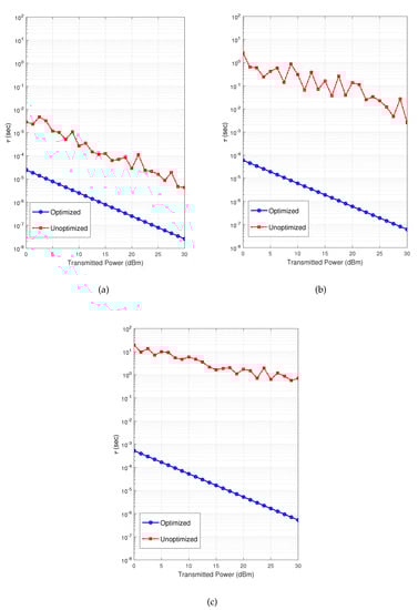
Figure 4. The transmission delay vs. transmission power at $n=500$, ${\alpha }_{y\left(0\right)}=2$, ${\alpha }_{y\left(1\right)}=3$, $r_f=100m$, and $r_c=500m$; (a) ${\alpha }_{x\left(0\right)}=2$, ${\alpha }_{x\left(1\right)}=3$; (b) ${\alpha }_{x\left(0\right)}=2$, ${\alpha }_{x\left(1\right)}=4$; (c) ${\alpha }_{x\left(0\right)}=3$, ${\alpha }_{x\left(1\right)}=4$.

The impact of the PLEs of the link from the FN to the cloud on the objective function is shown in Figure 5. The figure shows that the optimum value of p decreases as the links to the cloud experience higher PLEs, which is the opposite of the behavior observed in Figure 3 toward increasing the PLEs of the links between the ENs and the FNs. This can be explained by the fact that the higher PLEs results in a higher path loss of the links between the FNs and the cloud. Thus, the path loss of the direct links between some of the FNs and the cloud will be higher than the path loss if those nodes utilize other FNs to communicate with the cloud. Therefore, downgrading those FNs to ENs results in lower average transmission delay. Table 2 provides the values of the optimum p, $n_1$ and $n_0/n_1$ for the curves in Figure 5. The table indicates that when the links between the FNs and the cloud are subjected to higher path loss, a higher number of ENs are associated with each FN, which requires more computational capabilities and a larger bandwidth to be allocated to the FNs.

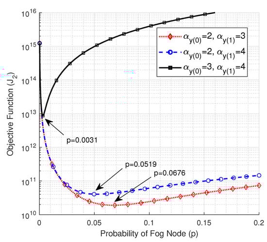
Figure 5. The objective function vs. p at $n=500$, ${\alpha }_{x\left(0\right)}=2$, ${\alpha }_{x\left(1\right)}=4$, $r_f=100m$, and $r_c=500m$.

Table 2. The optimum value of p, $n_1$, and $n_0/n_1$ at $n=500$, ${\alpha }_{x\left(0\right)}=2$, ${\alpha }_{x\left(1\right)}=4$, $r_f=100m$, and $r_c=500m$.

${\mathit{\alpha }}_{\mathit{y}\mathbf{\left(}\mathbf{0}\mathbf{\right)}}$	${\mathit{\alpha }}_{\mathit{y}\mathbf{\left(}\mathbf{1}\mathbf{\right)}}$	p	${\mathit{n}}_{\mathbf{1}}$	${\mathit{n}}_{\mathbf{0}}\mathbf{/}{\mathit{n}}_{\mathbf{1}}$
2	3	0.0676	33.78 ≈ 34	13.79
2	4	0.0519	25.97 ≈ 26	18.27
3	4	0.0031	1.57 ≈ 2	321.58

Figure 6 investigates the impact of the critical radius of the FN on the optimum number of FNs. The figure maintains that when the critical radius of the FN increases, the optimum value of p decreases, hence the fewer number of FNs are required to optimize the average transmission delay. This is owing to the larger number of ENs that reside within the critical radius where their links to the FN will be subjected to the low near-field PLE, which results in a lower average path loss that requires fewer FNs to optimize the performance.

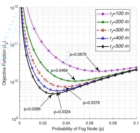
Figure 6. The objective function vs. p at $n=500$, ${\alpha }_{x\left(0\right)}=2$, ${\alpha }_{x\left(1\right)}=4$, ${\alpha }_{y\left(0\right)}=2$, ${\alpha }_{y\left(1\right)}=3$, and $r_c=500m$.

The impact of the critical radius of the cloud on the optimum number of FNs is illustrated in Figure 7. The figure shows that the optimum value of p, and as a consequence, the optimum number of FNs decreases with an increase in the critical radius of the cloud. The observed behavior is owing to the fact that as the critical radius of the cloud increases, more FNs reside within it with a lower path loss due to the low PLE of the near-field, which results in a lower transmission delay through those nodes. Thus, some of the FNs beyond $r_c$ are degraded to be ENs because their transmission delays through other FNs in the extended radius are less than transmission delays of the direct links between them and the cloud.

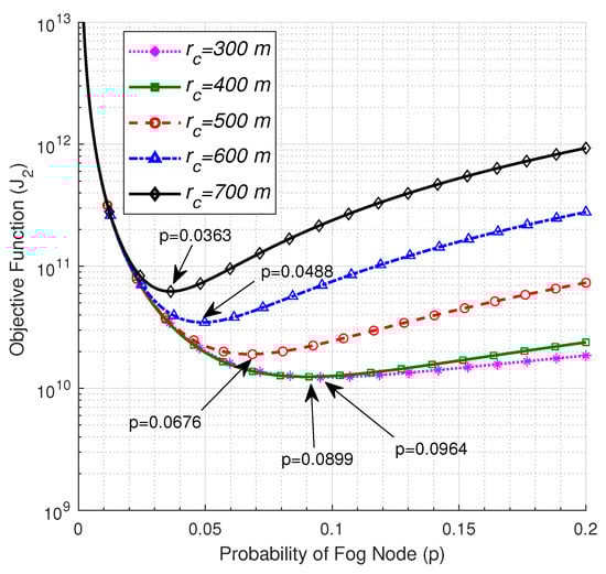
Figure 7. The objective function vs. p at $n=500$, ${\alpha }_{x\left(0\right)}=2$, ${\alpha }_{x\left(1\right)}=4$, ${\alpha }_{y\left(0\right)}=2$, ${\alpha }_{y\left(1\right)}=3$, and $r_f=100m$.

Figure 8 and Table 3 show the impact of the number of deployed nodes on the optimum number of FNs. We observe that increasing the number of deployed nodes n results in a decrease in the optimum value of p, which is due to the higher probability that there is a FN in the vicinity of the EN because of the lower probable separation distances between the nodes, and thus the lower probability that the node can be selected as a FN. Given that a lower probability of the FNs implies a higher number of ENs that are controlled by each FN, it means that higher computation and bandwidth resources are needed to be assigned to the FNs.

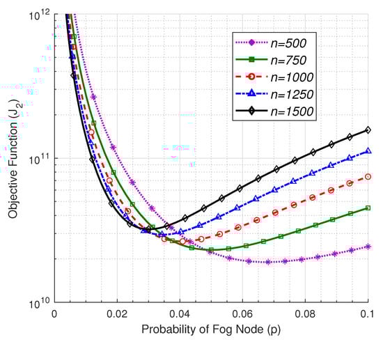
Figure 8. The objective function vs. p at ${\alpha }_{x\left(0\right)}=2$, ${\alpha }_{x\left(1\right)}=4$, ${\alpha }_{y\left(0\right)}=2$, ${\alpha }_{y\left(1\right)}=3$, $r_f=100m$, and $r_c=500m$.

Table 3. The optimum value of p, $n_1$, and $n_0/n_1$ at ${\alpha }_{x\left(0\right)}=2$, ${\alpha }_{x\left(1\right)}=4$, ${\alpha }_{y\left(0\right)}=2$, ${\alpha }_{y\left(1\right)}=3$, $r_f=100m$, and $r_c=500m$.

n	p	${\mathit{n}}_{\mathbf{1}}$	${\mathit{n}}_{\mathbf{0}}\mathbf{/}{\mathit{n}}_{\mathbf{1}}$
500	0.0676	33.7 ≈ 34	13.79
750	0.0502	37.65 ≈ 38	18.92
1000	0.0406	40.64 ≈ 41	23.63
1250	0.0345	43.13 ≈ 43	27.99
1500	0.0302	45.24 ≈ 45	32.11

6. Limitations and Future Work

The main objective of this paper is to optimize the number of FNs that minimize the transmission delay for uplink finite F-RAN. However, due to the small values of the propagation and processing delays compared to the transmission delay, both of them are omitted. Moreover, the impacts of the interference on the delay is not investigated for the sake of analytical tractability. In future studies, the impacts of interference, other sources of delay, and the mobility of the nodes on the optimum number of FNs for F-RAN will be investigated. However, such systems are very complex and thus the convexity of the optimization problem cannot be assured, nor a closed-form expression of optimum solution can be obtained. Therefore, finding the optimum solution using the heuristic optimization algorithms, such as Red Fox and Slime Mould, machine learning, or deep learning is highlighted as an open research direction.

7. Concluding Remarks

In this paper, we proposed a framework using stochastic geometry tool and exploiting MS-PLM to minimize the transmission delay in finite F-RANs by optimizing the number of FNs. We showed that the optimum number of FNs can be obtained by solving for the real root of a polynomial equation, the degree of which is determined by the far-field PLE of the link from the ENs to the FNs. Our simulation results show a significant reduction in the transmission delay gained by optimizing the number of FNs. Also, the impacts of the path loss parameters on the number of FNs have been analyzed. The results show that a small percentage of the deployed nodes are required to be selected as FNs to optimize the delay when the links to the FN experience a low path loss. Thus, additional bandwidth and computational capabilities are required at the FNs. However, this percentage increases as the PLEs of the links become higher. The results demonstrate that a larger number of FNs are needed to optimize the performance when the path loss of links to the FNs are higher than the path loss of the links to the cloud. Therefore, in these circumstances, centralized cloud networks can achieve better performance. The impact of the critical distance was also studied, which shows that the optimum number of FNs decreases when the critical distance increases. We also observe that the networks with densely deployed nodes require less percentage of them to be upgraded to FNs in order to minimize the transmission delay.

In general, the proposed approach can be applied to optimize the number of FNs in any IoT F-RAN, including NB-IoT and CAT-M1 networks, if the nodes selected as FNs are provided with higher computational and bandwidth resources. Finally, due to the accuracy attained by utilizing MS-PLM, our results provide a better insight into the design of F-RANs for more efficient utilization of FNs and virtualization of the cloud.

References

- Mouradian, C.; Naboulsi, D.; Yangui, S.; Glitho, R.H.; Morrow, M.J.; Polakos, P.A. A Comprehensive Survey on Fog Computing: State-of-the-Art and Research Challenges. IEEE Commun. Surv. Tutor. 2018, 20, 416–464. [Google Scholar] [CrossRef]
- Aleisa, M.A.; Abuhussein, A.; Sheldon, F.T. Access Control in Fog Computing: Challenges and Research Agenda. IEEE Access 2020, 8, 83986–83999. [Google Scholar] [CrossRef]
- Prokhorenko, V.; Ali Babar, M. Architectural Resilience in Cloud, Fog and Edge Systems: A Survey. IEEE Access 2020, 8, 28078–28095. [Google Scholar] [CrossRef]
- Habibi, P.; Farhoudi, M.; Kazemian, S.; Khorsandi, S.; Leon-Garcia, A. Fog Computing: A Comprehensive Architectural Survey. IEEE Access 2020, 8, 69105–69133. [Google Scholar] [CrossRef]
- Omoniwa, B.; Hussain, R.; Javed, M.A.; Bouk, S.H.; Malik, S.A. Fog/Edge Computing-Based IoT (FECIoT): Architecture, Applications, and Research Issues. IEEE Internet Things J. 2019, 6, 4118–4149. [Google Scholar] [CrossRef]
- Martinez, I.; Hafid, A.S.; Jarray, A. Design, Resource Management and Evaluation of Fog Computing Systems: A Survey. IEEE Internet Things J. 2020, 1-1. [Google Scholar] [CrossRef]
- Aslanpour, M.S.; Gill, S.S.; Toosi, A.N. Performance evaluation metrics for cloud, fog and edge computing: A review, taxonomy, benchmarks and standards for future research. Internet Things 2020, 12, 100273. [Google Scholar] [CrossRef]
- Habibi, M.A.; Nasimi, M.; Han, B.; Schotten, H.D. A Comprehensive Survey of RAN Architectures Toward 5G Mobile Communication System. IEEE Access 2019, 7, 70371–70421. [Google Scholar] [CrossRef]
- Naha, R.K.; Garg, S.; Georgakopoulos, D.; Jayaraman, P.P.; Gao, L.; Xiang, Y.; Ranjan, R. Fog Computing: Survey of Trends, Architectures, Requirements, and Research Directions. IEEE Access 2018, 6, 47980–48009. [Google Scholar] [CrossRef]
- Mukherjee, M.; Shu, L.; Wang, D. Survey of Fog Computing: Fundamental, Network Applications, and Research Challenges. IEEE Commun. Surv. Tutor. 2018, 20, 1826–1857. [Google Scholar] [CrossRef]
- Ni, J.; Zhang, K.; Lin, X.; Shen, X.S. Securing Fog Computing for Internet of Things Applications: Challenges and Solutions. IEEE Commun. Surv. Tutor. 2018, 20, 601–628. [Google Scholar] [CrossRef]
- Lin, H.; Zeadally, S.; Chen, Z.; Labiod, H.; Wang, L. A survey on computation offloading modeling for edge computing. J. Netw. Comput. Appl. 2020, 169, 102781. [Google Scholar] [CrossRef]
- Andrews, J.G.; Ganti, R.K.; Haenggi, M.; Jindal, N.; Weber, S. A primer on spatial modeling and analysis in wireless networks. IEEE Commun. Mag. 2010, 48, 156–163. [Google Scholar] [CrossRef]
- Haenggi, M.; Andrews, J.G.; Baccelli, F.; Dousse, O.; Franceschetti, M. Stochastic geometry and random graphs for the analysis and design of wireless networks. IEEE J. Sel. Areas Commun. 2009, 27, 1029–1046. [Google Scholar] [CrossRef]
- Azimi-Abarghouyi, S.M.; Makki, B.; Haenggi, M.; Nasiri-Kenari, M.; Svensson, T. Stochastic Geometry Modeling and Analysis of Single- and Multi-Cluster Wireless Networks. IEEE Trans. Commun. 2018, 66, 4981–4996. [Google Scholar] [CrossRef]
- Afshang, M.; Dhillon, H.S. Fundamentals of Modeling Finite Wireless Networks Using Binomial Point Process. IEEE Trans. Wirel. Commun. 2017, 16, 3355–3370. [Google Scholar] [CrossRef]
- Trinh, D.P.; Jeong, Y.; Shin, H. MIMO Capacity in Binomial Field Networks. IEEE Access 2017, 5, 12545–12551. [Google Scholar] [CrossRef]
- Srinivasa, S.; Haenggi, M. Distance Distributions in Finite Uniformly Random Networks: Theory and Applications. IEEE Trans. Veh. Technol. 2010, 59, 940–949. [Google Scholar] [CrossRef]
- Naghshin, V.; Rabiei, A.M.; Beaulieu, N.C.; Maham, B. Accurate Statistical Analysis of a Single Interference in Random Networks with Uniformly Distributed Nodes. IEEE Commun. Lett. 2014, 18, 197–200. [Google Scholar] [CrossRef]
- Chen, Y.; Zhu, J.; Shen, Y.; Jiang, X. Modeling the success transmission rate in Aloha MANETs with Binomial point process. In Proceedings of the 2015 Eighth International Conference on Mobile Computing and Ubiquitous Networking (ICMU), Hakodate, Japan, 20–22 January 2015; pp. 36–41. [Google Scholar] [CrossRef]
- Guo, J.; Durrani, S.; Zhou, X. Outage Probability in Arbitrarily-Shaped Finite Wireless Networks. IEEE Trans. Commun. 2014, 62, 699–712. [Google Scholar] [CrossRef]
- Tukmanov, A.; Ding, Z.; Boussakta, S.; Jamalipour, A. On the Broadcast Latency in Finite Cooperative Wireless Networks. IEEE Trans. Wirel. Commun. 2012, 11, 1307–1313. [Google Scholar] [CrossRef][Green Version]
- Afshang, M.; Dhillon, H.S. k-Coverage Probability in a Finite Wireless Network. In Proceedings of the 2017 IEEE Wireless Communications and Networking Conference (WCNC), San Francisco, CA, USA, 19–22 March 2017; pp. 1–6. [Google Scholar] [CrossRef]
- Balevi, E.; Gitlin, R.D. Optimizing the Number of Fog Nodes for Cloud-Fog-Thing Networks. IEEE Access 2018, 6, 11173–11183. [Google Scholar] [CrossRef]
- Heinzelman, W.R.; Chandrakasan, A.; Balakrishnan, H. Energy-efficient communication protocol for wireless microsensor networks. In Proceedings of the 33rd Annual Hawaii International Conference on System Sciences, Maui, HI, USA, 7 January 2000; Volume 2, p. 10. [Google Scholar] [CrossRef]
- Loscri, V.; Morabito, G.; Marano, S. A two-levels hierarchy for low-energy adaptive clustering hierarchy (TL-LEACH). In IEEE Vehicular Technology Conference; IEEE: Piscataway, NJ, USA, 2005; Volume 62, p. 1809. [Google Scholar]
- Younis, O.; Fahmy, S. Distributed clustering in ad-hoc sensor networks: A hybrid, energy-efficient approach. In IEEE INFOCOM 2004; IEEE: Piscataway, NJ, USA, 2004; Volume 1, p. 640. [Google Scholar]
- Youssef, A.; Younis, M.; Youssef, M.; Agrawala, A. WSN16-5: Distributed formation of overlapping multi-hop clusters in wireless sensor networks. In IEEE Globecom 2006; IEEE: Piscataway, NJ, USA, 2006; pp. 1–6. [Google Scholar]
- Youssef, M.; Youssef, A.; Younis, M. Overlapping Multihop Clustering for Wireless Sensor Networks. IEEE Trans. Parallel Distrib. Syst. 2009, 20, 1844–1856. [Google Scholar] [CrossRef]
- Bandyopadhyay, S.; Coyle, E.J. An energy efficient hierarchical clustering algorithm for wireless sensor networks. In IEEE INFOCOM 2003. Twenty-second Annual Joint Conference of the IEEE Computer and Communications Societies (IEEE Cat. No. 03CH37428); IEEE: Piscataway, NJ, USA, 2003; Volume 3, pp. 1713–1723. [Google Scholar]
- Zhang, X.; Andrews, J.G. Downlink Cellular Network Analysis With Multi-Slope Path Loss Models. IEEE Trans. Commun. 2015, 63, 1881–1894. [Google Scholar] [CrossRef]
- Munir, H.; Hassan, S.A.; Pervaiz, H.; Ni, Q.; Musavian, L. Resource Optimization in Multi-Tier HetNets Exploiting Multi-Slope Path Loss Model. IEEE Access 2017, 5, 8714–8726. [Google Scholar] [CrossRef]
- Gilani, S.Q.; Hassan, S.A.; Pervaiz, H.; Ahmed, S.H. Performance Analysis of Flexible Duplexing-enabled Heterogeneous Networks Exploiting Multi Slope Path Loss Models. In Proceedings of the 2019 International Conference on Computing, Networking and Communications (ICNC), Honolulu, HI, USA, 18–21 February 2019; pp. 724–728. [Google Scholar] [CrossRef]
- Yang, Y.; Sung, K.W.; Park, J.; Kim, S.; Kim, K.S. Cooperative transmissions in ultra-dense networks under a bounded dual-slope path loss model. In Proceedings of the 2017 European Conference on Networks and Communications (EuCNC), Oulu, Finland, 12–15 June 2017; pp. 1–6. [Google Scholar] [CrossRef]
- He, R.; Zhong, Z.; Ai, B.; Ding, J.; Guan, K. Analysis of the Relation Between Fresnel Zone and Path Loss Exponent Based on Two-Ray Model. IEEE Antennas Wirel. Propag. Lett. 2012, 11, 208–211. [Google Scholar] [CrossRef]
- Al-Samman, A.M.; Abd Rahman, T.; Al-Hadhrami, T.; Daho, A.; Hindia, M.N.; Azmi, M.H.; Dimyati, K.; Alazab, M. Comparative Study of Indoor Propagation Model Below and Above 6 GHz for 5G Wireless Networks. Electronics 2019, 8, 44. [Google Scholar] [CrossRef]
- Majed, M.B.; Rahman, T.A.; Aziz, O.A.; Hindia, M.N.; Hanafi, E. Channel Characterization and Path Loss Modeling in Indoor Environment at 4.5, 28, and 38 GHz for 5G Cellular Networks. Int. J. Antennas Propag. 2018, 2018, 9142367. [Google Scholar] [CrossRef]
- Hindia, M.N.; Al-Samman, A.M.; Bin Abd Rahman, T. Investigation of large-scale propagation for outdoor-parking lot environment for 5G wireless communications. In Proceedings of the 2016 IEEE 3rd International Symposium on Telecommunication Technologies (ISTT), Kuala Lumpur, Malaysia, 28–30 November 2016; pp. 14–18. [Google Scholar] [CrossRef]
- Hindia, M.; Al-Samman, A.; Rahman, T.; Yazdani, T. Outdoor large-scale path loss characterization in an urban environment at 26, 28, 36, and 38 GHz. Phys. Commun. 2018, 27, 150–160. [Google Scholar] [CrossRef]
- Lyu, K.; Rezki, Z.; Alouini, M. Accounting for Blockage and Shadowing at 60-GHz mmWave Mesh Networks: Interference Matters. In Proceedings of the 2018 IEEE International Conference on Communications (ICC), Kansas City, MO, USA, 20–24 May 2018; pp. 1–6. [Google Scholar] [CrossRef]
- Singh, S.; Mudumbai, R.; Madhow, U. Interference Analysis for Highly Directional 60-GHz Mesh Networks: The Case for Rethinking Medium Access Control. IEEE ACM Trans. Netw. 2011, 19, 1513–1527. [Google Scholar] [CrossRef]
- Pan, V. Algebraic complexity of computing polynomial zeros. Comput. Math. Appl. 1987, 14, 285–304. [Google Scholar] [CrossRef][Green Version]
Publisher’s Note: MDPI stays neutral with regard to jurisdictional claims in published maps and institutional affiliations. |
© 2020 by the authors. Licensee MDPI, Basel, Switzerland. This article is an open access article distributed under the terms and conditions of the Creative Commons Attribution (CC BY) license (http://creativecommons.org/licenses/by/4.0/).