Abstract
Smart grid technology is the next step to the evolution of classical power grids, providing robustness, reliability, and security throughout the network, enabling real-time management and control. To achieve these goals, distributed computing (microgrid concept) and intelligent control algorithms, tailored to the nature and needs of the network under study, are necessary. To deal with the vast diversity of power grids, being able to capture the dynamics of any given network, and create tools for network analysis, apparatus testing, and power grid management, an automatic design framework for real-time power system simulators is needed. In this article, a prototype of this approach is presented, employing Field Programmable Gate Array (FPGA) platforms due to their reconfigurability that enables low-power, low-latency, and high-performance designs, as a first attempt towards an open source platform, compatible with the majority of hardware design suites. It comprises two major parts: (i) a user-oriented section, built in Matlab/Simulink; and (ii) a hardware-oriented section, written in Matlab and Very High Speed Integrated Circuit (VHSIC)-Hardware Description Language (VHDL) code. To verify its functionality, two test power networks were given in a schematic format, analyzed through Matlab code and turned into dedicated hardware simulators with the aid of the VHDL template. Then, simulation results from Simulink and the prototype were compared for error estimation. The results show the prototype’s successful implementation with minimal resources utilization, high performance and low latency in the order of nanoseconds in Xilinx 6- and 7-series FPGAs, therefore proving its modularity and efficient use in many different scenarios, meeting low-latency/real-time requirements while enabling further smart grid research.
1. Introduction
Smart grid is a term used to describe the classical power grid enhanced with “intelligence” [1], in the sense that a logical layer (intelligence) is placed on top of the physical system, controlling its operation in real-time. This (logical) layer is composed of many different functional units, such as digital platforms, dedicated software and hardware accelerators which host the system’s logic, as well as from a trusted communication layer. Utilizing these resources, the smart grid integrates advanced computing and communication technologies in order to provide “smart” services to energy producers and consumers, while increasing the system’s reliability, security, efficiency, and resilience. In a smart grid framework (Figure 1) [2], the increasing energy demands of society, the problems and the constraints of the current power network infrastructure, the inclusion of numerous Renewable Energy Sources (RESs), the management of Distributed Energy Resources (DERs), and the control of a strongly heterogeneous system are crucial parameters that should be taken into account. Therefore, intelligence at the energy grid is of paramount importance for creating a modern, dynamic, and robust power system.

Figure 1.
Smart grid concept.
The ongoing research regarding smart grid technology faces many challenges of different difficulty levels and nature. This is due to the multidimensionality of the smart grid problem, which requires the combination of knowledge from different fields, e.g., power systems, communications, information technology, cyber-physical systems, Artificial Intelligence (AI), control theory, and economics. Most smart grid problems, e.g., optimal energy distribution, load balancing, load forecasting, transactive energy market, etc., require real-time monitoring and computing capabilities over the power grid so that system operators, utility companies, as well as consumers can monitor, process, and act upon important system data on-the-fly. For example, regarding the demand response management problem, especially when dealing with deregulated market models, the utility companies and the consumers need to solve game-like optimization problems to achieve balance between pricing and energy demand, while minimizing their respected costs [3,4]. The accurate real-time monitoring/prediction of the consumers’ energy demand eliminates this problem, by performing real-time simulation, possibly aided by conducting computations at the edge of the network. It can be easily inferred that smart grid problems require real-time simulation/monitoring, which facilitates the potential forthcoming needs of such dynamic environments.
Many state-of-the-art technologies have been considered to support the smart grid framework [5]. 5G technology has been proposed to meet the smart grid’s strict time requirements across its boundaries, to achieve real-time monitoring and control. Furthermore, Internet of Things (IoT) platforms are used in the smart grid context to define rules for communication, sharing and processing of data among sensors, smart meters, controllers and data centers; ease service applications’ design; and provide energy clients with ubiquitous access to smart services. For the “intelligent” part, many Machine Learning (ML) and deep learning techniques are available for high precision data analysis, while acceleration of such tasks to achieve real-time execution is possible thanks to the broad use of Field Programmable Gate Array (FPGA) platforms, which utilize special integrated circuits capable of addressing various, hard computing tasks due to their internal design, enabling them to be reconfigurable and to their inherent capability for even massive parallelism. However, there are still several issues to be addressed [6]. Some of the most critical are the grid’s complexity and size, and its security and dynamic management. To alleviate these problems, the microgrid concept is adopted. Microgrids—small-scale smart grids operating in a semi-autonomous manner—help to share/distribute the heavy network management workload to many small, easily managed and more secure networks, thus reducing the time for applying control actions and strengthening the overall system against cyber attacks.
Although microgrids are able to respond quickly to transient phenomena, the microgrid control logic should be customized to the underlying network to achieve best results. However, this is not a simple task as microgrids are expected to be highly diverse, therefore demanding a solution that provides flexibility. In that respect, we propose an automatic design framework for real-time power system simulators in the context of microgrid analysis, targeting FPGA platforms for their inherent parallelism, needed for achieving high performance and latency in the order of tenths of nanoseconds, and reconfigurability, which provides increased flexibility compared to other alternatives, e.g., General-Purpose Graphics Processing Units (GPGPUs). This concept of creating fully automated software platforms for providing simplicity and reducing production costs is not quite new. In power grid applications, software suites such as Matlab/Simulink, EMTDC/PSCAD [7], and EMTP [8,9] support this idea. In the context of real-time power system simulation, OPAL-RT [10] and Typhoon HIL [11] are two representative examples showcasing the increasing need for FPGA-based simulation platforms from the industry, which are, however, usually characterized of high cost. Additionally, in the last few years, researchers around the world have been trying to address this matter, creating a basis literature around this topic [12,13]. In that regard, our work is a first attempt to create a low-cost, full-solution platform targeting microgrids that provides the necessary tools, and enables the user to design custom power system hardware (through such a simulator) with much less effort. Moreover, this framework is the first step towards our vision of the design of a fully open source platform, which will contribute in the research towards power electronics, power grid design, and smart grid related topics, such as the enabling of intelligent, low latency microgrid control algorithms.
In this article, our automatic design framework for real-time power system simulators is proposed and a prototype implementation is provided. The logic diagram of the framework is presented in Figure 2. According to this, the power system simulator design is divided into two sections: the user-oriented and the hardware-oriented ones. In the user-oriented section, a General User Interface (GUI) is provided, where the schematic of any system under study can be created. In addition, a software library comprising component models and a network analysis algorithm are utilized in order to extract the system information in a compatible format for hardware implementation. Our network analysis algorithm simplifies the complexity of the simulation by applying graph optimizations where possible. Moreover, to further expand the library of compatible components towards creating a complete software toolkit, a library of complex component models and error estimation support are included. In the hardware-oriented section, a special module helps the user specify the fixed-point data representation for the simulation of the given network according to application-specific criteria, which usually are sufficient precision and low memory footprint. Lastly, a Hardware Description Language (HDL) template converts the user-oriented section fixed-point data to a customized real-time simulator targeting FPGA platforms, aiming at low memory, low computational resources, and high bandwidth [14,15,16,17], thus enabling Hardware-In-the-Loop (HIL) simulation for apparatus testing, facilitating the design of control algorithms, etc.
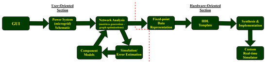
Figure 2.
Logic diagram of the proposed framework.
This article is organized as follows. In Section 2, the Numerical Integration Substitution (NIS) method, an essential technique in time-domain power system simulation, is presented, along with our custom optimizations and examples showcasing its use. In Section 3 and Section 4, the NIS-based network analysis and simulation algorithms are described, respectively, while in Section 5 our initial state estimation algorithm, created for achieving best-precision results, is briefly presented. In Section 6, the user-oriented section implementation in Matlab/Simulink is presented, while the hardware-oriented section implementation, written in Matlab and Very High Speed Integrated Circuit (VHSIC)-Hardware Description Language (VHDL) code, is shown in Section 7. Section 8 describes the results obtained with the proposed framework for two representative test cases, showcasing its low-cost implementation for two different platforms. Section 9 concludes the article.
2. NIS Method
The first and most crucial part of the simulator design is the way that the power system equations will be converted to an appropriate digital (or, in other words, discrete) format prior to being embedded in the simulator. There are several approaches to achieve this but, in our case, the NIS method is followed [18,19,20]. The NIS method, which is the basis of H. W. Dommel’s ElectroMagnetic Transients Program (EMTP) [21], is a way to numerically solve a system’s differential equations following a discrete analysis [22]. Through this method, the system components are analyzed into basic power system elements (resistors, inductors, and capacitors) via simple characteristic equations, which form a linear version of the original network, consisting of simple linear branches that can easily be discretized in the form of Norton equivalents (Figure 3).
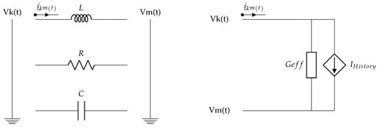
Figure 3.
Numerical Integration Substitution (NIS) method.
To use the NIS method, it is essential to define the numerical method with which the system equations will be discretized. For this purpose, the trapezoidal rule is chosen. The trapezoidal rule [23,24,25] has some special properties which make it stand out from the rest. It is able to track transients with sufficient precision, so long as the chosen numerical analysis time step t is considerably small, while being a low-cost, low-complexity method [26]. Thus, it is ideal for hardware implementation and satisfies our goals.
Assuming that the dynamics of many complex components in the power grid can be described as a combination of simple passive elements forming a network, the next step, as mentioned above, is to discretize those elements through the NIS method. To showcase the use of the method, the discretization of an inductor is shown (Figure 4).
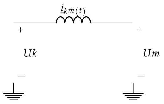
Figure 4.
Inductor.
The behavior of the inductor is expressed by the following differential equation, with respect to the notation in Figure 4:
Applying the trapezoidal rule yields:
As explicitly clarified in Equation (1), the characteristic equation of an inductor can be viewed as the sum of an instantaneous term and a history term. The former describes the immediate response of the component to a change in the voltage difference across its terminals, while the latter represents an inherent memory of the component preventing the change of its state. Equation (1) can then be represented by a Norton equivalent, as illustrated in Figure 5 [23], where the conductance G and the current source are the instantaneous and the history terms, respectively.
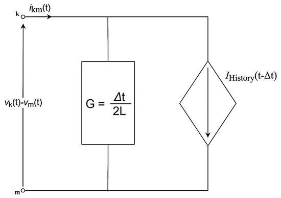
Figure 5.
Discrete model of the inductor.
Likewise, resistors and capacitors can be represented by their respected Norton equivalents. For readers’ convenience, the conductances and history currents of the basic elements are presented in Table 1.

Table 1.
Norton equivalents of basic elements.
To further simplify the analysis of a complex component or system, it is possible to extend the NIS method to series and parallel Resistor–Inductor (RI)/Resistor–Capacitor (RC) branches as well, reducing the number of branches and nodes in a circuit. In our framework, we make use of these graph optimizations to provide a hardware design of low memory footprint. The NIS method for the reduction of series and parallel RI/RC branches is visualized in Figure 6 and Figure 7.
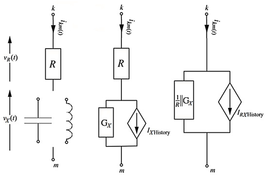
Figure 6.
Series Resistor–Inductor (RI)/Resistor–Capacitor (RC) Branch Reduction.
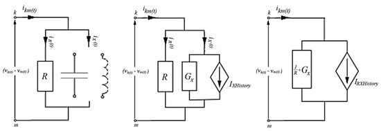
Figure 7.
Parallel RI/RC Branch Reduction.
The results are summarized in Table 2.
Table 2.
Norton equivalents of RI/RC branches.
The NIS method offers a simple way of creating digital models of complex components and its extensions make it possible to adapt to any simulation scenarios. In addition, it enables the representation of any model as a collection of constant data structures (matrices), due to the conversion of any network branch to a constant Norton equivalent. To defend our statement, the models of two complex components, a real linear transformer and a full-bridge power inverter, are shown in Figure 8 and Figure 9, respectively, along with their NIS equivalents. In the case of the transformer, the model comprises RI branches, which can be easily discretized to their NIS counterparts, and an ideal transformer of turns ratio a, which is characterized by the following system of equations (Equation (2)):
where are the voltage differences, are the currents, and are the number of turns in primary and secondary windings, respectively. In the case of the full-bridge power inverter, an NIS-based approach, the Associated Discrete Circuit (ADC) model [27,28,29,30,31], is used to convert power electronics, high-frequency switching components in the power grid, to their respected Norton equivalents. In both examples, simple discrete models of their associated continuous-time counterparts are derived. Non-linear elements can also be addressed through an NIS-like method, known as the piecewise linear approximation method [32], enabling real-time simulation of complex systems and electromagnetic phenomena [33,34,35,36,37,38,39,40,41]. Thus, NIS-based analysis of the diverse power grid is possible.
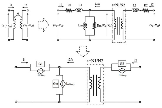
Figure 8.
Real linear transformer model and NIS-equivalent model.
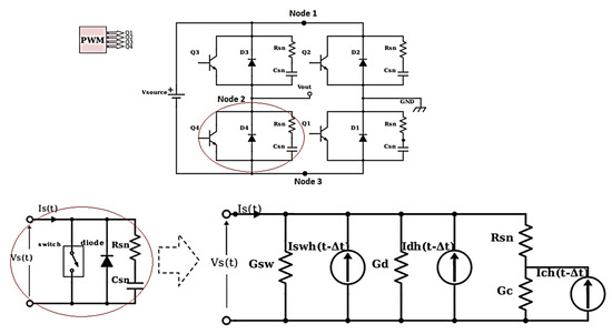
Figure 9.
Full bridge power inverter model and NIS analysis of power electronics using Associated Discrete Circuit (ADC) model.
3. NIS-based Network Analysis Algorithm
After defining the NIS method, its use and extensions, a NIS-based network analysis algorithm is presented in this section. To simulate the given (micro)grid, there are three main steps to follow. The first step is to convert the grid into a form which can be discretized. As stated above, this can be accomplished by modeling grid components as small networks of Resistor–Inductor–Capacitor (RIC) branches. Therefore, the whole grid can be discretized through NIS method in a simple manner. The second step is to collect the system equations and create a solvable mathematical problem. Having converted our study system into its NIS-based discretized form, which comprises conductance components, current sources, and possibly voltage sources, the behavior of the system can be expressed in the form of:
where G is the conductance matrix, is the vector of nodal voltages at time step t, is the vector of external current sources at time step t, and is the vector of history current sources at time step t. As stated in Section 2, the NIS method converts the system information to constant data structures, i.e. the G matrix, as well as the matrices of history current sources’ coefficients and branch conductances. In that way, complex systems comprising high-frequency switching components do not necessitate the computation of different matrices associated with possible system topologies. The thirdstep is to define the initial state of the system, which is addressed by our initial state estimation algorithm presented in Section 5. In general, this process includes the initialization of history current sources and external sources and the computation of the system equations for t = (at the start of the simulation). In this way, we prevent possible simulation errors associated with zero state and zero input responses of the system at t = , when transient phenomena emerge.
To showcase the network analysis algorithm, a test circuit (Figure 10) is converted to its discrete counterpart (Figure 11) with the above process. The test circuit consists of a voltage source with its internal resistor, a single-phase linear transformer in its model form, a resistive load and two RC branches. To analyze the network and transform it into Equation (3), the nodal analysis method is used. Having assigned id numbers to every node of the system, with the ground node being the reference node ( = 0V), and taking the component polarities into account, the process results in the mathematical system shown in Figure 12. In this figure, the constant conductance matrix G is shown analytically. It is worth mentioning that, to correctly transform the system into a mathematical equation, a property of the ideal transformer called mirroring effect is used. According to this, the impedance seen from one side of the transformer is a mirror image of the impedance connected at the other side. Therefore, it is possible to shift branches from one side of the ideal transformer to the other without error, after applying some modifications first, as shown in Figure 13.
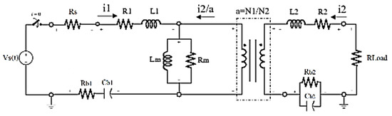
Figure 10.
Test circuit to be analyzed by NIS-based network analysis algorithm.
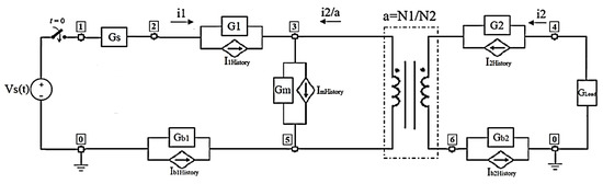
Figure 11.
Discrete version of the test circuit.
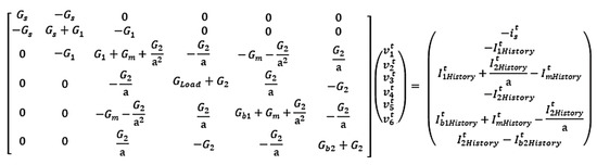
Figure 12.
Test circuit in the form of Equation (3).
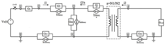
Figure 13.
Secondary side branch of ideal transformer referred to the primary.
4. NIS-based Simulation Algorithm
After employing the NIS-based network analysis algorithm, the simulation algorithm follows. The first step is the computation of the new values of the external sources and the history current sources, using the equations derived from the NIS method. The second step is the computation of the nodal voltages. From Equation (3):
where is the inverse conductance (resistance) matrix, which (for a given network topology) is constant throughout the simulation and needs to be calculated only once. In the case of voltage sources existing in the network, the process slightly changes. Equation (3) is rewritten in the form:
where matrix G is divided into four submatrices, each with a different subscript set, and the voltage/current vectors are divided into two subvectors. The subscripts U and K represent connections to nodes with unknown and known voltages, respectively. Then, Equation (5) is transformed into Equation (6), which returns the unknown nodal voltages’ values:
Equivalently, the currents of voltage sources are given by Equation (7):
The third step is to compute all the branch currents of the network at the present time step. This is due to the fact that the branch currents constitute valuable information about the network, since they are essential to the computation of the values of the history current sources at next time step. Knowing the conductance of the branches, the computation of the values of the history current sources and nodal voltages is a simple task. After the completion of these steps, the simulation cycle restarts until the predefined stop time.
It is worth noting that, in our design, the computation of the inverse matrices of the above equations is handled by the Singular Value Decomposition (SVD) method [42]. This method can be used to approximate the inverse of any conductance matrix G, even if it is ill-conditioned (its determinant is close to zero), which is essential for the simulation of many different systems.
5. Initial State Estimation Algorithm
In typical system simulation programs such as Simulink, during the configuration of the study system design and simulation parameters, an internal initial system state is defined. At the beginning of the simulation, at t = , the network is stimulated by external sources in an instant, such as turning on multiple switches simultaneously, therefore connecting the sources to the grid. During this process, the system is undergoing a transient state. That is, the initial conditions affect the system state after the very first time step. This is due to the rapid changes the system experiences from the “switching” effect.
To cope with this problem, a review in basic electrical circuit theory is mandatory. The “memory” components, the inductor and the capacitor, resist the sudden changes of their current and voltage, respectively. When a given system has an initial state before its stimulation by the sources, which means that the capacitors and inductors of the network have some initial voltage and current prior to their excitation, respectively, it shows some starting “inertia”. To solve this problem and be precise, during the first time step (t = ), it is suggested that all inductors be substituted by current sources of values equal to the initial currents. In the same way, all capacitors should be substituted by voltage sources of values equal to the initial voltages. The general concept is shown in an example in Figure 14. For zero initial state only, inductors can be thought as being open circuits whereas capacitors as short circuits. Having those facts in mind, the system under study can be reformed to its initial-state configuration and be solved afterwards with the help of the preestablished process (Equations (4), (6), (7)). After that, the analysis resumes in the standard way.
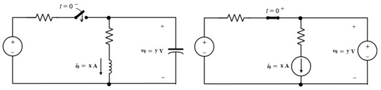
Figure 14.
Initial state model.
This methodology, called the initial state estimation algorithm, is an important asset to our framework, providing best-precision simulation results in any study case. The initial state derived by this algorithm is used below as the default starting point of the hardware simulator.
6. User-Oriented Section
Having covered the basic theoretical concepts for real-time power system simulation, our prototype implementation of an automatic design framework is presented here. The first part of our implementation is the user-oriented section. This section is dedicated to the user, the electrical or future smart grid engineer, providing tools and algorithms needed to draw a schematic, test a component model, and convert the schematic to a structure compatible with an HDL template. There are plenty of software tools and specialized libraries that can offer some of the capabilities needed for this section. In the context of this first attempt to design the framework and prove its functionality, we have chosen to work with existing software suites providing some basic GUI. One of the most known software suites that supports our needs regarding the design of the application architecture and provides numerous tutorials and educational documentation is Matlab. Matlab is an all-in-one solution that supports a wide variety of engineering problems and is widely spread across the academia [43]. Its simulation package, Simulink, is assumed to be very accurate, up-to-date, and supports problems of any kind, from fluid dynamics to electrical engineering [44].
In the context of our proposed framework, the concept was to make use of the Simulink GUI and a library called Simscape and create our custom Matlab code which reads the user’s input, the schematic of the system, and automatically extracts the required information to provide the needed services. The Simulink GUI consists of many simulation tools and functions, the most important tools of which—those used in the analysis—are the Model Configuration Parameters and the Library Browser. The Model Configuration Parameters, on the one hand, is the tool with which the simulation time and the Simulink solver options, needed for the model error estimation, are set. The Library Browser, on the other hand, is a (browser) tool providing access to all the Simulink libraries, including the Simscape library. The Simscape library includes a dedicated library for power systems called Specialized Technology [45], which features specialized power system models and enables an interface with other Simulink tools in a simple manner, creating a strong interconnection between Matlab and Simulink. Therefore, to achieve design simplicity and use up-to-date models, we opted for the Specialized Technology library and its models to be in the user-oriented section design. For our prototype, we used basic NIS-compatible one/three-phase passive components and dedicated components for simulating, measuring and displaying results. These components are shown in Figure 15.
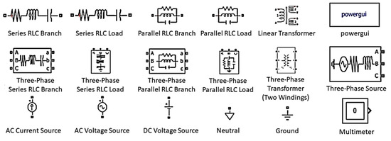
Figure 15.
Specialized Technology models used in the study.
The NIS-based (network analysis, simulation) and the initial state estimation algorithms, as well as the error estimation and HDL-compatible formatting ones, were all written into Matlab code. However, to make them accessible to the user in the form of Simulink plugins and executable by one click, we utilized the Simulink Subsystem component and created a library including the algorithms, customized as program execution buttons, called “auto_ps_sim_lib.slx”. The contents of this library can easily be included into a user design either by copying them into it or including the library into the Library Browser just by following Matlab instructions [46]. It is also possible for the user to include customized models complying with the NIS analysis into the library likewise to further extend the platform’s use for testing models and apparatus in an HIL way. All the Matlab code necessary for the deployment of the library and the library itself are available on Github [47].
A design paradigm is shown in Figure 16. The test network, presented in the upper half of the figure, consists of a sinusoidal current source, two resistive branches and a resistive load, one series RC branch, one parallel RI branch, and a real linear transformer. In the other half of the figure, a Multimeter component is shown to feed a Scope with the voltage and current of the resistive load, whose data are also logged in the Matlab workspace, as indicated by the notes in red colour above the vertical black bar. The Scope is used for displaying the data of interest. At the right side of the Scope component, two blocks can be spotted. These are our custom Simulink plugins, the use of which is also described in the red notes. The first block can be used to analyze the network, compare the Simulink simulation results with our custom Matlab code, and estimate the error. The second one converts the schematic to a VHDL-compatible format—using our HDL-compatible formatting algorithm—and provides possible error estimation between Simulink results and results obtained by the hardware design part of the software suite.
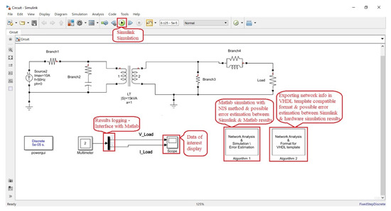
Figure 16.
Test network designed in Simulink General User Interface (GUI); important details and tools are marked in red.
7. Hardware-Oriented Section
The second part of our implementation is the hardware-oriented section. This section focuses on the actions that must be made for a study case to be embedded in an FPGA and run in real-time, while using minimum computational resources and memory. Taking into account the user’s specifications, this section acts as an interface between the user and the hardware implementation, removing any need for previous knowledge of HDLs from the user. It comprises two major modules: a module which helps the user specify a fixed-point data representation for the custom real-time hardware simulator and an HDL template which converts the schematic into a dedicated hardware architecture. In our prototype, we deployed the Fixed-Point Converter tool of Matlab [48] for the former module’s implementation, while the latter used our VHDL-compatible formatting algorithm and a VHDL template for the actual automatic hardware design.
To design an efficient hardware architecture, one crucial aspect is memory footprint, which affects greatly the power consumption of a chip. When dealing with hard computational problems, such as the precise simulation of a system’s behavior after a sequence of specific events, memory plays an important role. This is due to the number of memory cells, registers, flip-flops, etc. needed to achieve the problem-defined numerical accuracy. The number of bits in a digital design is not infinite, so as to withstand any numerical accuracy problem, nor can it cover a very wide range. In most cases, register size is constant throughout a design. This fixed bit length of digital values, while creating a consistent design, also minimizes power consumption due to reduced utilized hardware resources. In addition, numerical computations with fixed length and fixed data representation need less time than floating-point ones. Thus, creating an efficient simulator design calls for a global digital data representation, sufficient—according to the user—and in the same time small enough to limit power consumption.
In that respect, the Fixed-Point Converter tool of Matlab is a simple yet effective way for choosing the optimal fixed-point data representation. This tool is given the necessary computational tasks as inputs (in the form of functions), along with the network analysis and simulation script. Then, after specifying the fixed-point analysis properties, the tool runs the whole script and proposes fixed-point data representations for all the task variables. After choosing a global data representation with the help of the tool (by inspecting the range of the results), the tasks are converted into their fixed-point counterparts. The numerical accuracy of the fixed-point tasks can be tested either by the tool itself or by integrating the tasks within the network analysis and simulation script to create a fixed-point one for pre-implementation, and simulation purposes. Prior to the fixed-point analysis, a word length should be specified and data should be declared as signed data or else wrong hardware implementation will be derived. A sample configuration and fixed-point analysis results are shown in Figure 17 and Figure 18, respectively. In the latter figure, the “.m” files on the left are the tasks and the emts_FP.m testbench file is a copy of the network analysis and simulation script for fixed-point analysis purposes only.
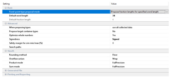
Figure 17.
Fixed-Point Converter Sample Configuration.
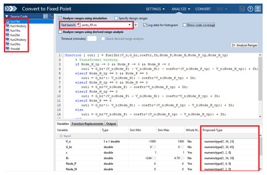
Figure 18.
Fixed-Point analysis results.
To be able to convert the information of a study system in a VHDL-compatible format, a dedicated script calls the network analysis algorithm to read and analyze the schematic, while applying graph optimizations, asks the user for the desired fixed-point properties (word and fraction length) and exports the network’s information in specific text files, coded in the desired binary format. All the important constant matrices or vectors (, history current coefficients, and branch conductances) follow the user’s specifications, while some information matrices about network connections or number of nodes/voltage (current) sources/fixed-point parameters are coded differently, since their purpose is to be used in the VHDL template only for information reasons. This script is deployed through the Simulink GUI as a plugin, as shown in Figure 16.
To be able to design a custom hardware architecture automatically for a power system simulator, our VHDL template is employed, which maps any power system simulator information to a predefined, customized, yet configurable hardware design. This hardware design can be viewed in Figure 19 in a block diagram form. It consists of five modules: the History Currents module computes the history current sources’ values, the Nodal Currents module computes the vector of currents needed in Equation (4), the Nodal Voltages module solves Equation (4), the Branch Voltages module transforms nodal to branch voltages, and the Branch Currents module computes the branch currents’ values.
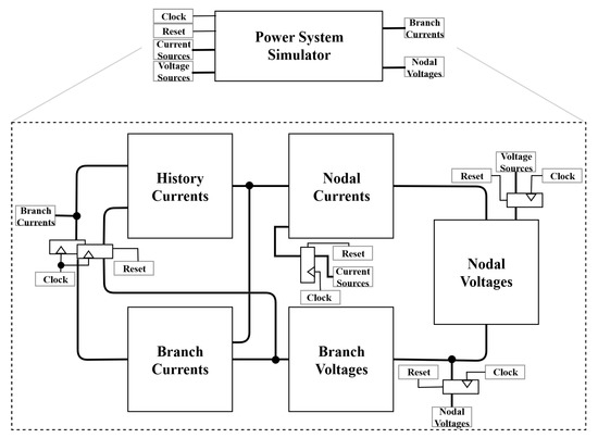
Figure 19.
Top-level block diagram of a power system hardware simulator.
Each module is designed to be extensible and adaptive to any study case. To achieve this in VHDL [49,50,51], which is a powerful, yet stiff hardware description language, our template consists of dedicated VHDL packages and functions to simplify the design and achieve the required flexibility. An important factor of the design is the Matlab-generated text files. When the template is synthesized via hardware design tools for a netlist to be created, the first step is for the text files to be read. Then, the network information is passed to the tools and can be used for appropriate design decisions. These decisions take place inside each module and are witnessed in the form of generated hardware. For example, let us focus on the case of “Nodal Voltages” module, where Equation (4) is solved. As shown in Figure 20, for an arbitrary network, each nodal voltage in the “Nodal Voltages” module is computed by a dedicated datapath associated with its mathematical expression. Our template ensures that no unused computations will occupy hardware resources (e.g., for multiplications/additions with zero elements) and that the datapath will not feature unnecessary processing stages that add delay to the computations.
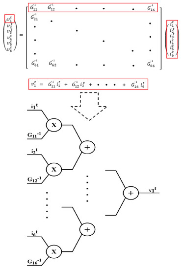
Figure 20.
Conversion of equations to hardware architecture.
The VHDL-compatible formatting algorithm can be found in the user-oriented section folder at Github [47], while the VHDL template is in the hardware-oriented section folder. Implementation instructions can be found online.
8. Results
8.1. First Test Case
8.1.1. Simulation
For the first test case, the Simulink model shown in Figure 16, analyzed in Section 6, was used as input to the Simulink GUI. For an analysis time step, we used , a relatively standard one for effectively capturing transient phenomena in power systems. Firstly, we simulated the model via the Simulink mathematical algorithms and the NIS method using double-precision (Matlab) operations. The purpose of this action was to test the NIS method prior to hardware implementation. To estimate the NIS method’s error, the voltage and current values of the network’s resistive load, derived by NIS method, were compared to the Simulink results. The results are shown in Figure 21 below:
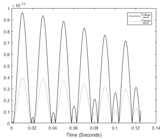
Figure 21.
Simulink-NIS method error results.
It can be easily derived that all the NIS-based algorithms and the component models used are implemented in the right way, as the error is close to zero.
After the system’s conversion to VHDL code with 34 bits word length and 19 bits fraction length (as dictated by the corresponding bit length estimation tool of our framework), the system was simulated using Vivado and ISE tools (hardware design software suites) with target devices the Zybo Z7-20 and the Virtex 6 ML605 Evaluation board, respectively. After collecting all the voltage and current values of the network’s resistive load from the corresponding tools in fixed-point format, the error was computed by comparing these results with the Simulink ones. The computation errors are shown in Figure 22.
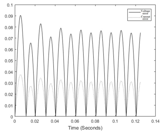
Figure 22.
Simulink-hardware error results.
The figure showcases the impact of the user-specified word length in the simulator’s accuracy. Depending on the system simulation requirements, the word length and the results’ accuracy may vary. Overall, the error results are acceptable as being below zero and can be further restricted according to the user’s wishes.
8.1.2. Hardware Design
As mentioned above, the hardware implementation of the first test case was successfully deployed in Virtex 6 ML605 Evaluation board [52], as well as in Zybo Z7-20 device [53]. An image of the implementation in Virtex 6’s FPGA is shown in Figure 23. In this image, the mapping of the physical hardware instances on the FPGA is indicated by the blue color.
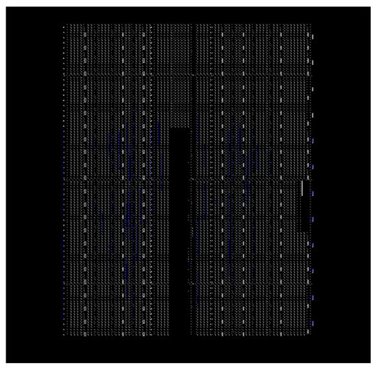
Figure 23.
FPGA mapping of the first test case simulator.
The utilization results of the hardware design in Zybo Z7-20 and Virtex 6 ML605 Evaluation board are shown in Table 3.
Table 3.
Utilization results.
In both cases, the implementation of the network simulation, by the proposed framework, results in a low-cost hardware design of low computational resources and memory usage. It is interesting to notice that, even in the case of Zybo Z7-20 board, which uses a smaller FPGA, the results show lower use of Digital Signal Processing (DSP) modules, resulting in a more efficient design.
Table 4.
Timing summary.
The results show that, in both cases, the designs for both target (FPGA) devices achieve latency close to 30 ns, maximum throughput of around 33 Msamples per second for an output of one sample, and operational frequency close to 33 MHz. This means that, for an analysis time step equal to , which tracks effectively the transients of a system, our hardware simulator is able to make an almost 30-min analysis of a simple microgrid-size circuit in 1 s, thus meeting network’s real-time requirements.
8.2. Second Test Case
8.2.1. Simulation
For the second test case, the Simulink model shown in Figure 24 was used as input to the Simulink GUI. This model is a variant of a typical Institute of Electrical and Electronics Engineers (IEEE) 5-Bus Model. It consists of two three-phase current sources, seven pi-modeled transmission lines, and four three-phase RI loads. For the analysis time step, we used , as in the previous scenario. Firstly, we simulated the Simulink mathematical algorithms and the NIS method using double-precision Matlab operations. To estimate the NIS method’s error, the voltage and current values of LOAD 5, derived by NIS method, were compared to the Simulink ones. The results are shown in Figure 25.
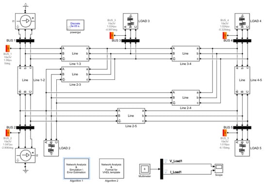
Figure 24.
Simulink model of the second test scenario.

Figure 25.
Simulink-NIS method error results for second test scenario.
It can be easily derived that all the NIS-based algorithms and the component models used are implemented in the right way, as the error is close to zero.
After the system’s conversion to VHDL code with 34 bits word length and 19 bits fraction length again, the system was simulated by Vivado and ISE tools for the Zybo Z7-20 and Virtex 6 ML605 Evaluation board, respectively. After collecting all the voltage and current values of the network’s LOAD 5 in fixed-point format, the error was computed by comparing these results with the Simulink ones. The computation errors are shown in Figure 26.
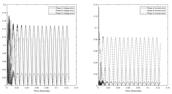
Figure 26.
Simulink-hardware error results for second test scenario.
It is obvious that the figures’ waveforms are matching, with the only difference being the slightly different accuracies of the results.
8.2.2. Hardware Design
The utilization results of the hardware design in Zybo Z7-20 and Virtex 6 ML605 Evaluation board are shown in Table 5.
Table 5.
Utilization results.
In both target devices, and as in the first test case, the implementation of the network simulation fits perfectly inside the FPGAs. Again, it could be noted that, in the case of Zybo Z7-20 board, equipped with a smaller size FPGA device (compared to the Virtex 6 device), we have much lower utilization of the DSP modules, thus indicating that in this test case too, Zybo handles more efficiently DSP designs.
Table 6.
Timing summary.
Using a similar analysis as in the previous test case, it can be easily derived from Table 6 that network’s real time requirements associated with this test case are also met.
9. Discussion
As stated in the Introduction, our work is a first attempt to create a full-solution platform that provides a simple, yet easy to use framework, featuring tools for drawing power systems and designing component models, while enabling simulations directly on hardware. It is designed for targeting mainly microgrid systems on FPGA platforms so as to make use of their reconfigurable characteristics and their inherent resources’ parallelism, to be able to create efficient hardware implementations on the same (low cost) device (Zybo Z7-20 is an indicative paradigm of such a low cost device), thus saving costs, especially since, as demonstrated through the test cases, a migrogrid-like structure can be readily accommodated in an FPGA device with low-medium resources such as the Zybo Z7-20 one. In addition, it is also compatible with many well known industry standard hardware design tools, such as Vivado and other platforms supporting the VHDL-93 standard. Therefore, it can be extended to target multiple FPGA devices as well. Moreover, this framework is the first step towards our open source platform vision, which will enable the design of smart (micro)grid-related applications and their implementation in real scenarios, outside of the laboratory, in low-cost FPGA platforms (especially when microgrids are involved, which is the current target of our framework), providing an accessible solution for smart grid researchers without the need of buying licenses for proprietary products. Beyond this, due to the high timing scores achieved and the real-time performance of the dedicated hardware, it can be easily deduced that smart (micro)grid applications requiring real-time simulation (computing) capabilities can be addressed without suffering from computation overheads.
Future work will be dedicated to the inclusion of more power system electronics’ models as well as non-linear elements in the framework. Next, further research will address the automatic hardware implementation, in the sense of how it can become more efficient while continuing to achieve low implementation cost and high performance. Moreover, a complete open source user-oriented section will be designed to promote the framework’s use and access so as to lead towards a fully open source platform. Finally, to fully utilize the hardware simulator and extend its use, standard interfaces could be designed for SoC-embedded system applications.
Author Contributions
Conceptualization, E.M., N.T., M.B., and A.B.; Data curation, E.M. and N.T.; Formal analysis, E.M. and N.T.; Investigation, E.M. and N.T.; Methodology, E.M., N.T., M.B., and A.B.; Project administration, M.B. and A.B.; Resources, M.B. and A.B.; Software, E.M. and N.T.; Validation, E.M. and N.T.; Visualization, E.M.; Writing—original draft, E.M.; and Writing—review and editing, M.B. and A.B. All authors have read and agreed to the published version of the manuscript.
Funding
The work of A. Birbas and N. Tzanis was partially co-funded by E.U and national funds the Regional Operation Programme “Western Greece 2014–2020” under the RIS3 Programme in “Microelectronics and Smart Materials” (Project: FPGAs 4SGs-MIS: 5021446). The work of M. Birbas and E. Mylonas was partially co-funded by E.U and national funds the Regional Operation Programme “Western Greece 2014–2020” under the RIS3 Programme in “Microelectronics and Smart Materials” (Project: DEEP-EVIoT-MIS: 5038640).
Conflicts of Interest
The authors declare no conflict of interest.
Abbreviations
The following abbreviations are used in this manuscript:
| FPGA | Field Programmable Gate Array |
| VHSIC | Very High Speed Integrated Circuit |
| VHDL | VHSIC-Hardware Description Language |
| RES | Renewable Energy Source |
| DER | Distributed Energy Resource |
| AI | Artificial Intelligence |
| LEM | Local Energy Market |
| IoT | Internet of Things |
| ML | Machine Learning |
| GPGPU | General-Purpose Graphics Processing Unit |
| GUI | General User Interface |
| HDL | Hardware Description Language |
| HIL | Hardware-In-the-Loop |
| NIS | Numerical Integration Substitution |
| EMTP | ElectroMagnetic Transients Program |
| RI | Resistor–Inductor |
| RC | Resistor–Capacitor |
| ADC | Associated Discrete Circuit |
| RIC | Resistor–Inductor–Capacitor |
| SVD | Singular Value Decomposition |
| DSP | Digital Signal Processing |
| IEEE | Institute of Electrical and Electronics Engineers |
References
- What Is the Smart Grid? Available online: https://www.smartgrid.gov/the_smart_grid/smart_grid.html (accessed on 3 September 2019).
- Thierry Legrand, La Numérisation de L’énergie (4/4): La RéVolution Industrielle des Smart Grids. Available online: https://les-smartgrids.fr/numerisation-energie-revolution-smart-grids (accessed on 2 July 2019).
- Chai, B.; Chen, J.; Yang, Z.; Zhang, Y. Demand Response Management With Multiple Utility Companies: A Two-Level Game Approach. IEEE Trans. Smart Grid 2014, 5, 722–731. [Google Scholar] [CrossRef]
- Apostolopoulos, P.A.; Tsiropoulou, E.E.; Papavassiliou, S. Demand Response Management in Smart Grid Networks: A Two-Stage Game-Theoretic Learning-Based Approach. Mobile Netw. Appl. 2018. [Google Scholar] [CrossRef]
- Kabalci, Y. A survey on smart metering and smart grid communication. Renew. Sustain. Energy Rev. 2016, 57, 302–318. [Google Scholar] [CrossRef]
- Watson, N.R.; Arrillaga, J. Power systems electromagnetic transients simulation. IEEE Power Energy 2003, 39, 449. [Google Scholar]
- Anaya-Lara, O.; Acha, E. Modeling and Analysis of Custom Power Systems by PSCAD/EMTDC. IEEE Trans. Power Deliv. 2002, 17, 266–272. [Google Scholar] [CrossRef]
- Zahavir, J.M.; krillaga, J.; Watson, N.R. Hybrid electromagnetic transient simulation with the state variable representation of HVDC converter plant. IEEE Trans. Power Deliv. 1993, 8, 1591–1598. [Google Scholar] [CrossRef]
- Durie, R.C.; Pottle, C. An extensible real-time digital transient network analyzer. IEEE Trans. Power Syst. 1993, 8, 84–89. [Google Scholar] [CrossRef]
- OPAL-RT Technologies, eFPGASIM. Available online: https://www.opal-rt.com/systems-efpgasim (accessed on 12 January 2020).
- Typhoon HIL. Available online: https://www.typhoon-hil.com (accessed on 12 January 2020).
- Dommel, H.W. Digital Computer Solution of Electromagnetic Transients in Single-and Multiphase Networks. IEEE Trans. Power Appar. Syst. 1969, 88, 388–399. [Google Scholar] [CrossRef]
- Farzanehrafat, A. Power Quality State Estimation. Ph.D. Dissertation, University of Canterbury, Christchurch, New Zealand, 2014. [Google Scholar]
- Mahseredjian, J. Computation of Power System Transients: Overview and Challenges. In Proceedings of the IEEE Power Engineering Society General Meeting, Tampa, FL, USA, 24–28 June 2007. [Google Scholar]
- Woods, R.; Mcallister, J.; Turner, R.; Yi, Y.; Lightbody, G. FPGA-Based Implementation of Signal Processing Systems; Wiley: Hoboken, NJ, USA, 2008. [Google Scholar]
- Chen, Y.; Dinavahi, V. FPGA-Based Real-Time EMTP. IEEE IEEE Trans. Power Deliv. 2009, 24, 892–902. [Google Scholar] [CrossRef]
- Parma, G.G.; Dinavahi, V. Real-time digital hardware simulation of power electronics and drives. IEEE Trans. Power Deliv. 2007, 22, 1235–1246. [Google Scholar] [CrossRef]
- Dommel, H.W. Electromagnetic Transients Program Theory Book; Bonneville Power Administration: Portland, OR, USA, 1986. [Google Scholar]
- Matar, M.; Bayoumi, A.M. An FPGA-Based Real-Time Simulator for the Analysis of Electromagnetic Transients in Electrical Power Systems. Ph.D. Dissertation, University of Toronto, Toronto, ON, Canada, 2009. [Google Scholar]
- Manitoba HVDC Research Center Inc. EMTDC User’s Guide; Manitoba HVDC Research Center Inc.: Winnipig, MB, Canada, 2004. [Google Scholar]
- Dommel, H.W. EMTP Theory Book; Microtran Power System Analysis Corporation: Vancouver, BC, Canada, 1996. [Google Scholar]
- Bari, A.; Jiang, J.; Saad, W.; Arunita, J. Challenges in the Smart Grid Applications: An Overview. Int. J. Distrib. Sens. Netw. 2014, 1–11. [Google Scholar] [CrossRef]
- Hollman, J.A. Step by Step Eigenvalue Analysis with EMTP Discrete Time Solutions New Methodology Test Cases; The University of British Columbia: Vancouver, BC, USA, 2006. [Google Scholar]
- Hall, G.; Watt, J. Modern Numerical Methods for Ordinary Differential Equations; Oxford University Press: New York, NY, USA, 1976. [Google Scholar]
- Selhi, H.; Christopoulos, C. Generalised TLM Switch Model for Power Electronics Applications. IEEE Proc. Sci. Meas. Technol. 1998, 145, 101–104. [Google Scholar] [CrossRef]
- Razzaghi, R.; Mitjans, M.; Rachidi, F.; Paolone, M. An automated FPGA real-time simulator for power electronics and power systems electromagnetic transient applications. Electr. Power Syst. Res. 2016, 141, 147–156. [Google Scholar] [CrossRef]
- Hui, S.Y.R.; Morrall, S. Generalised associated discrete circuit model for switching devices. IEEE Proc. Sci. Meas. Technol. 1994, 141, 57–64. [Google Scholar] [CrossRef]
- Tzanis, N.; Andriopoulos, N.; Proiskos, G.; Birbas, M.; Birbas, A.; Housos, E. Computationally Efficient Representation of Energy Grid-Cyber Physical System. In Proceedings of the IEEE Industrial Cyber-Physical Systems (ICPS), St. Petersburg, Russia, 15–18 May 2018. [Google Scholar]
- Tzanis, N.; Proiskos, G.; Birbas, M.; Birbas, A. FPGA-Assisted Distribution Grid Simulator. In Proceedings of the ARC 2018 Conference, Santorini, Greece, 8 April 2018. [Google Scholar]
- Marti, J.R.; Lin, J. Suppression of Numerical Oscillations in the EMTP. IEEE Trans. Power Syst. 1989, 9, 71–72. [Google Scholar] [CrossRef]
- Gear, C.W. Numerical Initial Value Problems in Ordinary Differential; Prentice Hall: Upper Saddle River, NJ, USA, 1971. [Google Scholar]
- Escamilla, A.C. Modelling Non-linear and Distributed Elements in Transient State Estimation. Ph.D. Dissertation, University of Canterbury, Christchurch, New Zealand, 2015. [Google Scholar]
- Marti, J.R.; Linares, L.R. Real-time EMTP-based Transients Simulation. IEEE Trans. Power Syst. 1994, 9, 1309–1317. [Google Scholar] [CrossRef]
- Sybille, G.; Giroux, P. Simulation of FACTS Controllers Using the MATLAB Power System Blockset and Hypersim Real-time Simulator. In Proceedings of the IEEE Power Engineering Society Winter Meeting, New York, NY, USA, 27–31 January 2002. [Google Scholar]
- Devaux, O.; Levacher, L.; Huet, O. An Advanced and Powerful Real-time Digital. IEEE Trans. Power Deliv. 1998, 13, 421–426. [Google Scholar] [CrossRef]
- Pak, L.; Faruque, M.O.; Nie, X.; Dinavahi, V. A Versatile Cluster-based Realtime Digital Simulator for Power Engineering Research. IEEE Trans. Power Syst. 2006, 21, 455–465. [Google Scholar] [CrossRef]
- Hollman, J.A.; Marti, J.R. Real Time Network Simulation with PC-Cluster. IEEE Trans. Power Syst. 2003, 18, 563–569. [Google Scholar] [CrossRef]
- Kuffel, R.; Beum, Y.; Lee, J. Overview of the Development and Installation of KEPCO Enhanced Power System Simulator. In Proceedings of the 2000 IEEE Power Engineering Society Winter Meeting, Vasteras, Sweden, 23–27 January 2000. [Google Scholar]
- Abourida, S.; Belanger, J.; Dufour, C. Real-Time HIL Simulation of a Complete PMSM Drive at 10’s Time Step. In Proceedings of the 11th European Conference on Power Electronics and Applications, Dresden, Germany, 11–14 September 2005. [Google Scholar]
- Dinavahi, V. Real-Time Digital Simulation of Switching Power Circuits. Ph.D. Dissertation, University of Toronto, Toronto, ON, Canada, 2000. [Google Scholar]
- Strunz, K. Flexible Numerical Integration for Efficient Representation of Switching in Real Time Electromagnetic Transients Simulation. IEEE Trans. Power Deliv. 2004, 19, 1276–1283. [Google Scholar] [CrossRef]
- Jia, Y.-B. Singular Value Decomposition. 2013. Available online: http://web.cs.iastate.edu/~cs577/handouts/svd.pdf (accessed on 30 November 2019).
- The Math Works Inc. Matlab Optimization Toolbox—User’s Guide. Available online: https://www.mathworks.com/help/pdf_doc/optim/optim_tb.pdf (accessed on 4 August 2019).
- The Math Works Inc. Simulink—Getting Started Guide. Available online: https://www.mathworks.com/help/pdf_doc/simulink/sl_gs.pdf (accessed on 4 August 2019).
- The Math Works Inc. Simscape Electrical—User’s Guide (Specialized Power Systems). Available online: https://www.mathworks.com/help/pdf_doc/physmod/sps/powersys.pdf (accessed on 26 July 2019).
- The Math Works Inc. Add Libraries to the Library Browser. Available online: https://www.mathworks.com/help/simulink/ug/adding-libraries-to-the-library-browser.html (accessed on 20 November 2019).
- Auto Design Framework for Real-time Power System Simulators. Available online: https://github.com/lefmylonas/auto_power_system_simulator.git (accessed on 7 January 2020).
- The Math Works Inc. Fixed-Point Designer—User’s Guide. Available online: https://www.mathworks.com/help/pdf_doc/fixedpoint/FPTUG.pdf (accessed on 7 August 2019).
- Armstrong, J.R.; Gray, F.G. VHDL Design Representation and Synthesis, 2nd ed.; Prentice Hall PTR: Upper Saddle River, NJ, USA, 2000. [Google Scholar]
- Pellerin, D.; Taylor, D. VHDL Made Easy; Prentice Hall: Upper Saddle River, NJ, USA, 1997. [Google Scholar]
- Vahid, F. VHDL for Digital Design; John Wiley & Sons: Hoboken, NJ, USA, 2007. [Google Scholar]
- ML605 Hardware User Guide, UG534 (v1.9). 26 February 2019. Available online: https://www.xilinx.com/support/documentation/boards_and_kits/ug534.pdf (accessed on 15 October 2019).
- Zybo Z7 Board Reference Manual, Revised 21 February 2018. Available online: https://reference.digilentinc.com/_media/reference/programmable-logic/zybo-z7/zybo-z7_rm.pdf (accessed on 12 October 2019).


© 2020 by the authors. Licensee MDPI, Basel, Switzerland. This article is an open access article distributed under the terms and conditions of the Creative Commons Attribution (CC BY) license (http://creativecommons.org/licenses/by/4.0/).