Abstract
This study proposes an approaching method of identifying sea fog by using Geostationary Ocean Color Imager (GOCI) data through applying a Convolution Neural Network Transfer Learning (CNN-TL) model. In this study, VGG19 and ResNet50, pre-trained CNN models, are used for their high identification performance. The training and testing datasets were extracted from GOCI images for the area of coastal regions of the Korean Peninsula for six days in March 2015. With varying band combinations and changing whether Transfer Learning (TL) is applied, identification experiments were executed. TL enhanced the performance of the two models. Training data of CNN-TL showed up to 96.3% accuracy in matching, both with VGG19 and ResNet50, identically. Thus, it is revealed that CNN-TL is effective for the detection of sea fog from GOCI imagery.
1. Introduction
Sea fog is one of the major reasons for maritime accidents in Korea because of poor visibility (less than 1 km) [1,2,3]. It deters navigators from keeping a lookout for surrounding ships and obstacles [4]. Sea fog occupies 29.5% of total maritime accidents such as marine traffic, naval operations, and fisheries [5]. Most current vessels use facsimile to confirm sea fog’s existence. However, the broadcasting and nowcasting of sea fog events have limitations due to their temporal and spatial characteristics. For instance, the number of coastal meteorological stations is not enough to represent sea fog across the oceans [6]. In this regard satellite remote sensing technology could be a decent method for monitoring sea fog with its wide coverage.
There are a number of studies on sea fog detection from satellite imagery. Those studies are mainly categorized in accordance with the types of sensors, such as temperature and optical reflection. For detection of sea fogs with thermal characteristics, the Moderate-resolution Imaging Spectroradiometer (MODIS) has been widely used [7,8,9,10]. Bendix (2005) discriminated fog by observing the albedo of low stratus [7]. Zhang and Yi (2013) detected sea fog by comparing the relative frequency of brightness temperature (Tb) between sea fog and low stratus [8]. Wu and Lee (2014) classified sea fog and stratus cloud by Tb differences in the thermal infrared channel [9]. Jeon et al. (2016) conducted spectral analysis on sea fog, low stratus, mid-high clouds, wavelength, and corresponding reflectance [10]. Infrared (IR) imagery were also used to detect fog. Ellrod et al. (1995) developed a technique to identify sea fog and low cloud at night by using the IR channel of the Geostationary Operational Environmental Satellite (GOES), regardless of using sea surface temperature (SST) [11]. Lee et al. (1997) created stratus and fog products by using long- and short-wave channels both from GOES and Advanced Very High-Resolution Radiometer (AVHRR) [12]. Cermak and Bendix (2008) detected fog and stratus by using Meteosat 8 Spinning-Enhanced Visible and Infra-Red Imager (SEVIRI) through calculating the difference of radiances for respective gross cloud, snow, ice cloud, and small droplets of fog and stratus [13].
Fog detection can also be done by using optical characteristics of objects in the images. Dual-Channel Difference (DCD) is the most-used method to discriminate sea fog from low stratus because sea fog has small Tb difference rather than mid and high cloud in 3.7 and 11 μm (IR) channels [14,15,16,17]. Geostationary Ocean Color Imager (GOCI) also has been used for detecting sea fogs. Yuan et al. (2016) used indices for GOCI band radiances to discern land and sea, middle- and high-level clouds, fog and stratus [18]. Those indices identify sea fog by the characteristics of individual pixels; thus in some cases cloud pixels can also be incorrectly recognized as sea fog because those do not consider the relationship with adjacent pixels. On the contrary, there have been studies using Region of Interest (ROI) from GOCI images. Rashid and Yang (2016, 2018) estimated and predicted sea fog movement using the ROI of sea fogs from GOCI imagery and Weather Research and Forecasting-based simulated wind data [19,20]. However, the ROIs were generated manually based on visual observation of sea fogs in images [20].
Studies on sea fog detection were not limited to thermal and optical characteristics. Wu et al. (2015) developed a method to discriminate sea fog by using Cloud-Aerosol Lidar with Orthogonal Polarization (CALIOP), and evaluated the result through comparison with MODIS [21]. Heo et al. (2008) used IR and shortwave IR from GOES-9, MTSAT-1R for DCD, and QuikSCAT wind data for wind speed criteria [4].
Sea fog detection by using the optical characteristics of independent pixels cannot consider near pixels, and subsequently incorrectly identifies cloud as sea fog. The ROI of sea fog also needs manual work. If detection of sea fog could be automated with hourly satellite imagery instead of manual ROI preperation, it could enhance sea fog nowcasting. Thus, this paper introduces the sea fog identification method using GOCI with a Convolutional Neural Network Transfer Learning (CNN-TL) model that has been trained with an ImageNet dataset [25]. The model differentiates sea fog from clouds and other objects to solve overfitting which often appears in a small dataset. Alike preceding studies, GOCI satellite imageries were adopted in this study because of its hourly observations, wide coverage, as well as its high resolution [18,19,20].
2. Data
GOCI is one of the three payloads onboard the Communication, Ocean and Meteorological Satellite (COMS). GOCI generates images eight times per day with hourly intervals from 00:15 to 07:45 UTC. Its coverage is 2500 × 2500 km, covering Korea as well as Japan and East China.Its spatial resolution is 500 m [22]. GOCI has 8 spectral bands covering visible to near-IR wavelengths of the light spectrum. Bands 1 to 6 are visible bands, and Bands 7 and 8 are Near IR (NIR) bands. The central wavelengths of the bands are Band 1: 412 nm; Band 2: 443 nm; Band 3: 490 nm; Band 4: 555 nm; Band 5: 660 nm; Band 6: 680 nm; Band 7: 745 nm; and Band 8: 865 nm. Bands 1 to 5 are generally used to study biological matters such as chlorophyll, and Bands 6 to 8 are used for atmospheric matters such as atmospheric correction and fluorescence signals [23].
For this study GOCI L1B data were used which are readily geometrically and radiometrically corrected. Training and test image datasets of sea fogs and other objects in images inside the oceanic regions around the Korean Peninsula were extracted for the dates of 1, 2, 3, 15, 18, and 21 March, 2015, when sea fogs are very common during the Korean spring season.
To make training and test datasets specific RGB compositions (R-8, G-2, B-1) were used, in which sea fog has a pink and soft surface texture while clouds have a relatively white and coarse texture. Thus, sea fog become well distinguishable from clouds. Areas for datasets were 100 × 100 pixels, representing 50 × 50 km, made by selecting the position of sea fog, clouds, and other objects manually as shown in Figure 1. For training and test datasets 100 and 20 images were generated, respectively, following classes as sea fog, cloud, and others, and sorted into each training and test folder where both folders have respective sub-folders named as respective classes. Figure 2 shows the representative images of sea fog and cloud as true color composites. An RGB composition (R-6, G-4, B-2) is applied to compare the texture difference between two classes.
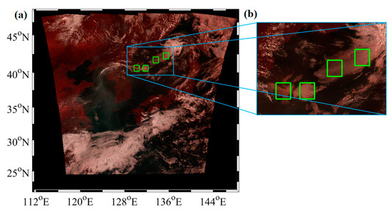
Figure 1.
Setting dataset areas in a Geostationary Ocean Color Imager (GOCI) image. Image is composited with an RGB composition (R-8, G-2, B-1): (a) land, cloud, seafog and oceans have colors red, bright pink, dark pink, and black, respectively; (b) green squares are the areas of sea fog dataset extraction, with a size of 100 × 100 pixels.
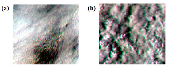
Figure 2.
Representative images for sea fog and clouds: (a) sea fog has a fine texture; (b) cloud has a coarse surface texture. These two images have RGB composition (R-6, G-4, B-2) to show texture differences, while Figure 1 shows color difference.
3. Methodology
3.1. CNN-TL Model
Traditional CNN usually requires a long time to be developed, needs a huge computation effort, and needs to be dedicated to a specific task at a time. Transfer learning overcomes that high time consumption and solve isolation through utilizing data acquired for one task to solve related another work [24].
In this study two popular CNN models were used, named VGG19 and ResNet50. These two CNN models were pre-trained with 1.2 million images from the ImageNet dataset [25]. Thus, these two models have high performance when identify images with fewer layers than that of traditional models. To classify sea fog 1,000 classes of original CNN models were reduced into 3 classes, which are sea fog, cloud, and others. The new model of this study was created in a Python-based Keras. Python is one of the free program languages, and Keras is a framework that provides an easy and high-quality Application Programming Interface (API) to construct an efficient deep learning model with a little coding [24]. Parameters of the CNN models used in this research are shown in Table 1.

Table 1.
Parameters of the Convolution Neural Network (CNN) model used in this study.
A training epoch is how many iterations the model were tuned from the data. The batch size is how many images were used to tune in one batch. An optimizer is a mathematical approach to reduce the error rate from the model. Adam was chosen as the optimizer because it is computationally efficient and has little memory requirement [26]. Learning rate controls how quickly or slowly a model is tuned. An activation function is required to make the model non-linear.
3.2. Band Combination
As training and test datasets five kinds of band combinations were used, viz. 3 bands (R-8, G-2, B-1), 5 bands (Band 2, 3, 4, 6, and 7), 5 bands and ratio, and 5 bands and average. The 3 bands were chosen because they can properly reflect the optical characteristics and features of sea fog, and were used for dataset extraction. The 5 bands are the union of three bands (R-7, G-3, B-2) and the other three bands (R-6, G-4, B-2) which are widely used for sea fog detection. The ratio is calculated by Equation (1) and represents the ratio of the shortest wavelength to the longest wavelength. The average is calculated by Equation (2) and represents the middle/high level cloud deduction index [10]. RGB is only applicable for 3-bands composites. Thus, in this study 5 bands were stacked as a 5-dimensional array, regardless of assigning color. 5 bands and ratio, and 5 bands and average mean the sixth array which was calculated by Equations (1) and (2), and is stacked on the 5-bands arrays.
The 3-bands images were used here which can be recognized by transfer learning. The other combinations were not available for transfer learning because ImageNet does not support images over 3 bands. The overall process of sea fog identification is described in Figure 3.
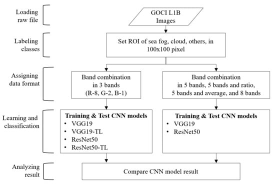
Figure 3.
Overall process of sea fog identification. The 5 bands consist of Band 2, 3, 4, 6, and 7. Transfer Leanring (TL) was applied to both VGG19 and ResNet50 only for 3-bands combination.
4. Results
The training accuracy and test accuracy were evaluated as shown in Figure 4. The model was first tuned, and 100 training images were identified for every class, then the training accuracy for same training images were calculated. Test accuracy was used to find out the model’s overfitting by separating training model and test images. The trained model classifies 20 new test images for every class, then evaluates test accuracy. Accuracy was calculated by using the Equation (3).
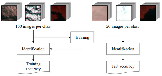
Figure 4.
Difference between training accuracy and test accuracy. Training accuracy means that identical images are used both for training and testing, while test accuracy represents that the trained model identifies independent images that were not used in training.
The test accuracy shows the model’s generalization performance and can represent the reliability of the model. To ensure the stability of performance we checked the trends of accuracy according to the number of epochs as shown in Figure 5.
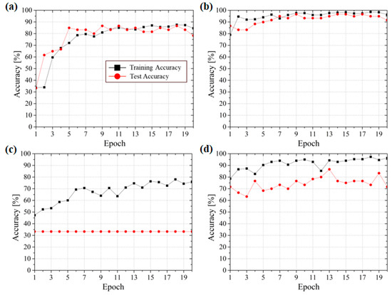
Figure 5.
Accuracy of training and test for CNN and CNN-TL with 3-bands images. Black squares and red circles represent training accuracy and test accuracy, respectively: (a) VGG19 has high and stable accuracy for both training and test; (b) TL enhances its performance from the beginning of VGG19; (c) ResNet50 shows lower values because the model was not trained enough; (d) TL remarkably increases the accuracy of ResNet50.
The confusion matrix explains how the two models correctly identified objects in Figure 6.
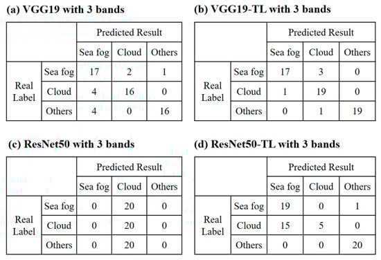
Figure 6.
Confusion matrix of sea fog, cloud, and others for CNN models with 3-bands images: (a,b) show that VGG 19 has high accuracy of identification; (c) represents that ResNet50 is not stable because the model was not trained enough with its small number of training datasets; (d) shows TL enhances the identification performance of the ResNet50 model.
VGG19 and VGG19-TL properly classify every class in this study. However, ResNet50 shows the lowest performance among the four models (VGG19, VGG19-TL, ResNet50, and ResNet50-TL). This shows the importance of setting an identical number of images for each class before training and classification. If a specific class had an overwhelming number of images, the model classifies every image into the class which has a large number of images, and the result seems to show high performance due to the good model. That is, the accuracy 33.3%, resulting from the classification of 3 classes which have the same number of images, shows that the ResNet50 was not trained enough with its low number of training images, and does not classify the images correctly. Although TL improved ResNet50’s accuracy, it still has a problem with discriminating clouds from sea fog. Table 2 shows the performance of the identification for every model in this study.
Table 2.
Results of identification according to the number of bands and models.
Both VGG19 and ResNet50 models with TL have higher accuracies than those without TL. The VGG19 model performed well both with and without TL. Although ResNet50-TL shows high identification performance, ResNet50 shows a lower training accuracy than VGG19. There are 4 cases where the test accuracy is higher than training accuracy. These results could come with fewer datasets and epochs, as well as the function of shuffle, which reads training datasets in random orders and dropouts to prevent the model from overfitting. The four conditions made random results.
5. Discussion
In this study we conducted an identification experiment, varying whether TL is applied, using only 100 images for training per class, in five kinds of band combination, setting 20 epochs. When it comes to TL, VGG19 and ResNet50 were remarkably enhanced for sea fog identification. As shown in Figure 5 the training and test accuracy increases as the epoch number increases. On the other hand, ResNet50 retains a lower test accuracy with a value of 33.3%, while training accuracy has ascending trends. Thus, it is revealed that VGG19-TL is suitable for sea fog identification. VGG19, in most cases, had higher accuracy than ResNet50. The VGG19 and ResNet50 models showed high identification accuracy when TL was applied. On the other hand, the two models without TL showed underfit. This means that the models were not trained well enough to make an identification, and their performance had poor accuracy.
In terms of band combination, 3 bands (R-8, G-2, B-1) showed higher identification performances than 5 bands, 5 bands and ratio, 5 bands and average, and 8 bands images, as in Table 2. Unlike the thought that the more information, the higher the accuracy, this result shows that increasing the number of bands is not a way of improving the model’s performance.
We used 20 epochs to train the models because this can show stable accuracy trends as in Figure 5. Twenty epochs are not enough in general identification cases. Although higher performance can be obtained by increasing the number of epochs, it consumes more computation time. Thus, determining the epoch is important to get both identification effectiveness and time efficiency.
6. Conclusions
From this study it is revealed that selecting specific bands is more effective for enhancing the performance of sea fog identification from GOCI images, rather than increasing the number of bands for datasets. Further, CNN-TL showed higher accuracy than traditional CNN. Thus, the use of CNN-TL, where possible, is better to obtain convincing results.
The VGG19 model, among the two CNN models, has a small difference in accuracy between the model with TL and without TL. Thus, it can be concluded that the VGG19 with 3 bands is suitable for sea fog identification.
Some improvements can still be made for CNN model. Firstly, there needs to be another experiment for identification, with different models and bigger datasets. Secondly, the models need the detection of sea fog with localization so that they can show where sea fog is in the GOCI image by creating bounding boxes. Thirdly, the models need to generate a new image that only shows the sea fog from the GOCI image through segmentation of sea fog. Lastly, they need to predict the sea fog movement from the time-lapse images using recurrent CNN.
Author Contributions
Conceptualization, C.-S.Y.; methodology, J.E.; software, S.K. and J.E.; validation, H.-K.J. and S.K.; formal analysis, S.K. and J.E.; investigation, H.-K.J., S.K. and J.E.; resources, C.-S.Y.; data curation, H.-K.J.; writing—original draft preparation, H.-K.J.; writing—review and editing, H.-K.J.; visualization, H.-K.J., S.K. and J.E.; supervision, C.-S.Y.; project administration, C.-S.Y.; funding acquisition, C.-S.Y. All authors have read and agreed to the published version of the manuscript.
Funding
This research is a part of the project entitled “Development of Ship-handling and Passenger Evacuation Support System”, “Construction of Ocean Research Stations and their application Studies”, “Technology Development for Practical Applications of Multi-Satellite Data to Maritime Issues”, funded by the Ministry of Oceans and Fisheries, Korea.
Conflicts of Interest
The authors declare no conflict of interest.
References
- Gultepe, I.; Hansen, B.; Cober, S.; Pearson, G.; Milbrandt, J.; Platnick, S.; Taylor, P.; Gordon, M.; Oakley, J. The fog remote sensing and modeling field project. Am. Meteorol. Soc. 2009, 90, 341–359. [Google Scholar] [CrossRef]
- Gultepe, I.; Kuhn, T.; Pavolonis, M.; Calvert, C.; Gurka, J.; Heymsfield, A.J.; Liu, P.; Zhou, B.; Ware, R.; Ferrier, B.; et al. Ice fog in arctic during FRAM-ICE fog project: Aviation and nowcasting applications. Am. Meteorol. Soc. 2014, 95, 211–226. [Google Scholar] [CrossRef]
- Koračin, D.; Dorman, C.E.; Lewis, J.M.; Hudson, J.G.; Wilcox, E.M.; Torregrosa, A. Marine fog: A review. Atmo. Res. 2014, 143, 142–175. [Google Scholar] [CrossRef]
- Heo, K.; Kim, J.; Shim, J.; Ha, K.; Suh, A.; Oh, H.; Min, S. A Remote Sensed Data Combined Method for Sea Fog Detection. Korean J. Remote Sens. 2008, 24, 1–16. [Google Scholar]
- Heo, K.Y.; Park, S.; Ha, K.J.; Shim, J.S. Algorithm for sea fog monitoring with the use of information technologies. Meteorol. Appl. 2014, 21, 350–359. [Google Scholar] [CrossRef]
- Yuan, Y.; Qiu, Z.; Sun, D.; Wang, S.; Yue, X. Daytime sea fog retrieval based on GOCI data: A case study over the Yellow Sea. Opt. Express 2016, 24, 787–801. [Google Scholar] [CrossRef] [PubMed]
- Bendix, J.; Thies, B.; Cermak, J.; Nauß, T. Ground fog detection from space based on MODIS daytime data-a feasibility study. Weather Forecast 2005, 20, 989–1005. [Google Scholar] [CrossRef]
- Zhang, S.P.; Yi, L. A comprehensive dynamic threshold algorithm for daytime sea fog retrieval over the Chinese adjacent seas. Pure Appl.Geophys. 2013, 170, 1931–1944. [Google Scholar] [CrossRef]
- Wu, X.; Li, S. Automatic Sea Fog Detection over Chinese Adjacent Oceans Using Terra/MODIS Data. Int. J. Remote Sens. 2014, 35, 7430–7457. [Google Scholar] [CrossRef]
- Jeon, J.-Y.; Kim, S.-H.; Yang, C.-S. Fundamental Research on Spring Season Daytime Sea Fog Detection Using MODIS in the Yellow Sea. Korean Soc. Remote Sens. 2016, 32, 339–351. [Google Scholar] [CrossRef]
- Ellrod, G.P. Advances in the detection and analysis of fog at night using GOES multispectral infrared imagery. Weather Forecast 1995, 10, 606–619. [Google Scholar] [CrossRef]
- Lee, T.F.; Turk, F.J.; Richardson, K. Stratus and fog products using GOES-8-9 3.9-μm data. Weather Forecast 1997, 12, 664–677. [Google Scholar] [CrossRef]
- Cermak, J.; Bendix, J. A novel approach to fog/low stratus detection using Meteosat 8 data. Atmos. Res. 2008, 87, 279–292. [Google Scholar] [CrossRef]
- Hunt, G.E. Radiative properties of terrestrial clouds at visible and infra-red thermal window wavelengths. Q. J. R. Meteorol. Soc. 1973, 99, 346–369. [Google Scholar]
- Eyre, J.; Brownscombe, J.; Allam, R. Detection of fog at night using Advanced Very High Resolution Radiometer (AVHRR) imagery. Meteorol. Mag. 1984, 113, 266–271. [Google Scholar]
- Turner, J.; Allam, R.; Maine, D. A Case Study of the Detection of Fog at Night Using Channel 3 and 4 on the Advanced Very High Resolution Radiometer (AVHRR). Meteorol. Mag. 1984, 115, 285–290. [Google Scholar]
- Ahn, M.; Sohn, E.; Hwang, B. A New Algorithm for Sea Fog/Stratus Detection Using GMS-5 IR Data. Adv. Atmos. Sci. 2003, 20, 899–913. [Google Scholar] [CrossRef]
- Jeon, J.-Y. Preliminary Study on Spring Season Daytime Sea Fog Detection Method Using MODIS in the Yellow Sea. Master’s Thesis, Korea Maritime and Ocean University, Busan, Korea, August 2016. [Google Scholar]
- Rashid, A.; Yang, C.-S. A simple sea fog prediction approach using GOCI observations and sea surface winds. Remote Sens. Lett. 2018, 9, 21–31. [Google Scholar] [CrossRef]
- Rashid, A.; Yang, C.-S. Estimation of Sea Fog Movement Using Satellite Data and 20-km WRF Wind Field in the East Sea from February to April in 2014. J. Coast. Disaster Prev. 2016, 3, 128–134. [Google Scholar]
- Wu, D.; Lu, B.; Zhang, T.; Yan, F. A method of detecting sea fogs using CALIOP data and its application to improve MODIS-based sea fog detection. J. Quantum Spectrosc. Radiat. 2015, 153, 88–94. [Google Scholar] [CrossRef]
- Yang, C.S.; Song, J.H. Geometric performance evaluation of the Geostationary Ocean Color Imager. Ocean Sci. J. 2012, 47, 235–246. [Google Scholar] [CrossRef]
- Ryu, J.-H.; Han, H.-J.; Cho, S.; Park, Y.-J.; Ahn, Y.-H. Overview of Geostationary Ocean Color Imager (GOCI) and GOCI Data Processing System (GDPS). Ocean Sci. J. 2012, 47, 223–233. [Google Scholar] [CrossRef]
- Sarkar, D.; Bali, R.; Ghosh, T. Hands-On Transfer Learning with Python; Packt: Berminghan, UK, 2018. [Google Scholar]
- ImageNet. Available online: http://www.image-net.org (accessed on 30 December 2019).
- Kingma, D.P.; Ba, J.L. Adam: A method for Stochastic Optimization. arXiv 2014, arXiv:1412.6980. [Google Scholar]


© 2020 by the authors. Licensee MDPI, Basel, Switzerland. This article is an open access article distributed under the terms and conditions of the Creative Commons Attribution (CC BY) license (http://creativecommons.org/licenses/by/4.0/).