Machine Learning Based Approaches for Modeling the Output Power of Photovoltaic Array in Real Outdoor Conditions

Abstract

It is important to investigate the long-term performances of an accurate modeling of photovoltaic (PV) systems, especially in the prediction of output power, with single and double diode models as the configurations mainly applied for this purpose. However, the use of one configuration to model PV panel limits the accuracy of its predicted performances. This paper proposes a new hybrid approach based on classification algorithms in the machine learning framework that combines both single and double models in accordance with the climatic condition in order to predict the output PV power with higher accuracy. Classification trees, k-nearest neighbor, discriminant analysis, Naïve Bayes, support vector machines (SVMs), and classification ensembles algorithms are investigated to estimate the PV power under different conditions of the Mediterranean climate. The examined classification algorithms demonstrate that the double diode model seems more relevant for low and medium levels of solar irradiance and temperature. Accuracy between 86% and 87.5% demonstrates the high potential of the classification techniques in the PV power predicting. The normalized mean absolute error up to 1.5% ensures errors less than those obtained from both single-diode and double-diode equivalent-circuit models with a reduction up to 0.15%. The proposed hybrid approach using machine learning (ML) algorithms could be a key solution for photovoltaic and industrial software to predict more accurate performances.

1. Introduction

Due to the high increase of petroleum prices and imposed politics on industrial countries to reduce CO₂ levels, the use of renewable sources to produce energy has become an obligation. Accordingly, different solutions are used to cover energy needs while respecting clean and eco-friendly requirements [1]. Generally, wind, hydro, and solar sources of energy show an appropriate solution ensuring green electricity for diverse industrial and domestic applications. In particular, photovoltaic systems display a good balance between investment cost and performance [2].

The modeling task is a substantial procedure to analyze the electrical performances of the photovoltaic (PV) cell/module/array. Equivalent-circuit models are mainly implemented to predict the long-term potential of the photovoltaic device. Single-diode model (SDMs) and double-diode models (DDMs) represent the most used configurations [3]. Furthermore, the single-diode model is less complicated compared to the double-diode configuration; this is because of the limited number of parameters needed. The SDM requires five while DDM requires seven [4]. To achieve a high level of accuracy, several modeling processes have been developed. Either based on analytical or metaheuristic methods, the predicted performances of PV modules are still limited in accuracy due to the use of only one equivalent-circuit configuration (SDM or DDM) to electrically model the PV cell behavior. This limitation is demonstrated under the variation of solar irradiance and temperature [4,5]. Nevertheless, several studies discuss the influence of climatic conditions. Ishaque et al. claimed that the single-diode model exhibits modest performances compared to the DDM under low-irradiance variation; this is demonstrated by comparing generated current voltage (I–V) curves and adopting both models with experimental data [4,6]. Also, Ishaque et al. proved that the DDM is more accurate under partial shading conditions. Et-torabi et al. [7] adopted iterative methods and proved that SDM can reach high accuracy for high irradiance and low-temperature levels. In addition, Villalva et al. demonstrated that the SDM is more simple and pertinent for all variations [8]. Chaibi et al. proposed a combination of SDM and DDM according to climatic changes in order to improve accuracy and get high prediction performance [5].

In the last years, machine learning (ML) techniques have been widely adopted to estimate the long-term performances, and predict the output power, of PV plants [9,10]. Theocharides et al. [11] assessed the PV generation using three ML techniques, such as artificial neural network (ANN), support vector machine (SVM), and regression tree. The results proved that the ANN presents high accuracy compared to other examined algorithms. Several approaches based on SVMs have been proposed to forecast the PV output power. Shi et al. [12] predicted the PV power for a 20 kW grid-connected PV installation located in China according to weather classifications (rainy, foggy, cloudy, and sunny). An SVM used real outdoor data of solar irradiance and ambient temperature to forecast PV power generation 24 h ahead [13]. In another study [14], an SVM combined with three-dimensional wavelet transform predicted the PV power of distributed PV plants using historical time series data. Furthermore, Wang et al. proposed a short-term power prediction using the gradient boost decision tree (GBDT) algorithm adopting historical weather data together with PV output powers [15].

The main objective of this work is to present a machine learning based approach that combines both single-diode and double-diode equivalent-circuit models according to climatic conditions in order to predict the output PV power with high accuracy. Therefore, the performances of single-diode and double-diode models are investigated under different levels of solar irradiance and ambient temperature. A comparison of the PV power estimated by using two equivalent-circuit models with real recorded data is performed in this study. Later, the effectiveness of machine learning techniques to select models according to corresponding accuracy is assessed. Therefore, an approach based on ML classification algorithms is proposed to prioritize single-diode and double-diode equivalent-circuit models for a given solar irradiance and temperature. Six classification algorithms, such as classification trees (coarse tree), k-nearest neighbors (cubic), discriminant analysis (quadratic), Naïve Bayes (kernel), support vector machines (Gaussian), and classification ensembles (boosted trees-AdaBoost) are implemented to categorize SDMs and DDMs into specific “classes” in order to predict the output PV power using real outdoor operating conditions. The accuracy of all classifiers is evaluated under real outdoor conditions of a 114 kW grid-connected PV plant located in Southern Italy. The novelty of this work is to evaluate the effectiveness of the proposed approach; the classification algorithms are able to select between single- and double-diode equivalent-circuit models according to different levels of solar irradiance and temperature, in order to ensure high accuracy in the output power predicting.

The present paper is arranged as follows: PV modeling and the classification algorithms are presented in Section 2. Then, the proposed hybrid approach is introduced in Section 3. The results and discussion are presented in Section 4. Finally, we give some conclusions.

2. Materials and Methods

2.1. PV Cell Modeling

To evaluate the electrical behavior of the PV device (cell), plenty of equivalent-circuit models are proposed. In the literature, there are two configurations widely used. Namely, the single- and the double-diode model.

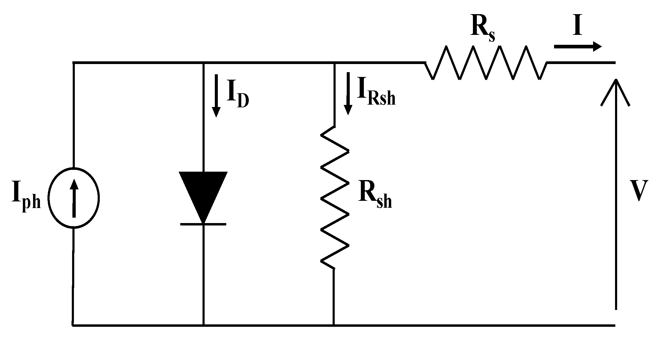
2.1.1. Single-diode Model

This model is developed by adding a series and a shunt resistance to the ideal model to represent the losses of the module [16]. By applying the Kirchhoff laws on the scheme in Figure 1, the output current of the PV panel is given by the following Equation [16]:

$$I=I_{ph}-I_{os}\left\{\exp \left[A\left(V+{IR}_s\right)-1\right]\right\}-\frac{V+R_{s}I}{R_{sh}} ,$$

(1)

where, $I_{ph}$ is the light-generated current, $I_{os}$ is the diode saturation current, and $R_s$ and $R_{sh}$ are respectively the series and the shunt resistance. The value of $A$ depends on the thermal voltage $V_t=\raisebox{1ex}{$kT$}\!\left/ \!\raisebox{-1ex}{$q$}\right.$ and is expressed as follows:

$$A=\frac{1}{V_t{N}_{\mathrm{cell}}} ,$$

(2)

γ is the ideality factor of the diode, and $N_{\mathrm{cell}}$ represents the number of cells that compose the PV module.

2.1.2. Double-Diode Model

As another configuration to model the PV cell, the double-diode is an improvement of what was claimed about the single-diode accuracy [17]. Recently, the DDM has become a primary solution for several authors due to its improvements especially at low-irradiances [4,18]. This model considers two diodes in parallel with the current source as shown in Figure 2, and the output current is given by Equation (3):

$$I=I_{ph}-I_{os1}\left\{\exp \left[A_1\left(V+{IR}_s\right)-1\right]\right\}-I_{os2}\left\{\exp \left[A_2\left(V+{IR}_s\right)-1\right]\right\}-\frac{V+R_{s}I}{R_{sh}} ,$$

(3)

where, $A_1$ and $A_2$ depend respectively on the values of the ideality factor of each diode (${\gamma }_1$ and ${\gamma }_2$) and cell temperature. In addition, $I_{os1}$ and $I_{os2}$ are the saturation current of each diode separately.

The second step of PV cell modeling is to evaluate the unknown parameters of Equations (1) and (3). The number of parameters to determine depends on the used equivalent-circuit model (e.g., five parameters for the single-diode model ($I_{ph},I_{os},R_s,R_{sh},$), and seven parameters for the double-diode model ($I_{ph},I_{os1},I_{os2},R_s,R_{sh}{,}_1,{}_2$, ${\gamma }_1$, ${\gamma }_2$)) [5].

To estimate these unknown parameters, many techniques are proposed using different approaches. Whether it is a numerical, analytical, or metaheuristic based method [19,20,21], most of these approaches use I–V experimental data or datasheet information to simplify the estimation of the parameters. For this reason, the photo-generated current is generally calculated using Equation (4) [22]:

$$I_{ph}=\left[I_{sc}+K_i\left(T-298.15\right)\right]\frac{\lambda }{1000} ,$$

(4)

where, $I_{sc}$ is the short-circuit current, $K_i$ is the temperature coefficient related to $I_{sc}$, and $\lambda$ and $T$ are respectively the solar irradiance level and cell temperature.

2.1.3. Maximum Power Point

The maximum power point (MPP) represents the optimal operating of the PV module regardless of climate variations [23]. Mathematically at this point, the derivative of PV power with respect to PV voltage is expressed as follows:

$$\frac{\partial P}{\partial V}=I+V\frac{\partial I}{\partial V}=0,$$

(5)

In order to compute the maximum power point for both adopted equivalent-circuit models, the current expressions in Equations (1) and (2) are calculated using Equation (5). Then, the optimal currents of the single-diode and double-diode models are respectively expressed by the following equations:

$$I_{\mathrm{MPP}}=\left(V_{\mathrm{MPP}}-R_s{I}_{\mathrm{MPP}}\right)\left\{{AI}_{os}\exp \left[A\left(V_{\mathrm{MPP}}+R_s{I}_{\mathrm{MPP}}\right)\right]+\raisebox{1ex}{$1$}\!\left/ \!\raisebox{-1ex}{$R_{sh}$}\right.\right\} ,$$

(6)

$$\begin{gathered} I_{\mathrm{MPP}}=\left(V_{\mathrm{MPP}}-R_s{I}_{\mathrm{MPP}}\right)\{I_{os1}{A}_1\exp \left[A_1\left(V_{\mathrm{MPP}}+R_s{I}_{\mathrm{MPP}}\right)\right] \\ +I_{os2}{A}_2\exp \left[A_2\left(V_{\mathrm{MPP}}+R_s{I}_{\mathrm{MPP}}\right)\right]+\raisebox{1ex}{$1$}\!\left/ \!\raisebox{-1ex}{$R_{sh}$}\right.\} , \end{gathered}$$

(7)

where, $V_{\mathrm{MPP}}$ and $I_{\mathrm{MPP}}$ are respectively the PV output voltage and current at the maximum power point. The $V_{\mathrm{MPP}}$ and $I_{\mathrm{MPP}}$ coordinates are then used to estimate the output power $P_{\mathrm{MPP}}= V_{\mathrm{MPP}}\ast I_{\mathrm{MPP}}$ for both adopted equivalent-circuit models.

In order to obtain the maximum power from a PV plant, a maximum power point tracking (MPPT) algorithm controls and adjusts the operating voltage to reach the maximum output power. MPP losses occur when the MPPT is not able to find the MPP rapidly. Typical MPP loss values are lower than 0.5%. Furthermore, the operating voltage of the PV array depends on the DC cable length, cross-section, and temperature that can lead to current and power losses, and the connection of modules in series can cause the mismatching between the I–V characteristics of the module (mismatch losses). In the present work, when modeling PV, estimation of the MPPT and DC losses are not considered.

2.2. Adopted Machine Learning Algorithm

Supervised machine learning (ML) techniques are able to predict the response for a given measurement set of the predictor variables on the base of a model built on a known observation set noted as the training dataset.

Classification algorithms are a type of supervised ML technique in which an algorithm learns to separate the data into specific “classes” in order to predict categorical responses [24]. The most popular classification algorithms include [25]:

• classification trees (coarse tree)
• k-nearest neighbors (cubic)
• discriminant analysis (quadratic)
• Naïve Bayes (kernel)
• support vector machines (Gaussian)
• classification ensembles (boosted trees-AdaBoost)

2.2.1. Classification Trees

The classification tree technique also noted as a decision tree is one of the common approaches applied in data mining to predict the class response for a given observation by using specific predictor variables [26]. The classification tree learning maps the observations as a tree structure to model its target value [27]. In the tree, each node represents a feature and each path corresponds to what is associated. The decision tree learner can identify each node that classifies the best value of the feature within the dataset according to some criterion. The terminal nodes are marked according to the classes into which the instances are to be classified. During the testing, the value of the instance is compared with the value labeled at each path (branch). If the value at the node matches the value of the node then the classification will continue through the path until it meets the terminal node as shown in Figure 3 [28]. The terminal leaf nodes are shown as orange and yellow squares according to the classes. In each tree, the instance is shown in a blue path. In Figure 3a–c the tree predicts the yellow class, unlike in Figure 3d the instance is in the orange class, so the classifier will assign it to the yellow class by a 3 to 1 majority voting.

2.2.2. k-Nearest Neighbors

The k-nearest neighbors algorithm (kNN) is a ML method applied for classification where an instance represents a point in a d-dimensional space and each dimension corresponds to one of the d features. So, the instances which present the same properties would be close to each other in the d-dimensional space [29]. In order to predict the class, the kNN algorithm finds k nearest instances by computing the distance between them. The predicted class is represented by the minimum distance among instances. The Euclidean distance is usually applied as the distance metric [30,31]. The k-nearest neighbor classification algorithm is listed in Appendix A. Figure 4 shows the kNN classification concept. The green instance will be assigned to the blue class for k = 1. For k = 3 it will be classified as the blue class by a 2 to 1 majority and finally, it will be assigned to the orange class by 3 to 2 cases for k = 5. Therefore, the k-nearest-neighbors classifier assigns to a test sample the majority class of its k-nearest training samples.

2.2.3. Discriminant Analysis

Discriminant analysis (DA) finds a predictive equation based on independent variables to classify the instances into classes [32]. Discriminant analysis is very similar to regression analysis, where the dependent variables become the independent variables in the discriminant analysis. The mathematical formulation is presented in Appendix A. It can be considered as dimensionality reduction technique, reducing the sample space into a smaller dimension while retaining as much information as possible. Discriminant analysis can be distinguished into two categories in according to the boundary between the classes: linear discriminant analysis (LDA) or quadratic discriminant analysis (QDA) [33]. LDA adopts the coordinate axes to transform data by reducing the two-dimensional space into a one-dimensional space using a linear boundary. The QDA can be considered as an extension to the LDA. It classifies two or more classes by a quadratic model as a surface.

2.2.4. Naïve Bayes

Naïve Bayes classification algorithm is one of the most popular statistical learning methods based on the Bayes theorem related to the conditional probability, predicting the most probable class.

Given an instance and its occurring probability $P\left(d\right)$, the Bayes theorem says:

$$P\left(c_i|d\right)=\frac{P\left(d|c_i\right)\ast P\left(c_i\right)}{P\left(d\right)} ,$$

(8)

where:

• $P\left(c_i|d\right)$ is the probability of the instance d being in the class c_i;
• $P\left(d|c_i\right)$ is the probability of observing d in a domain where c holds;
• $P\left(c_i\right)$ is the prior probability of c_i;

The Naïve Bayes classifier computes the probability of each instance for all classes in c and selects the class c_i with the highest probability (Figure A1). Generally, the features are assumed to have a Gaussian probability distribution. When the features do not follow a Gaussian distribution, the kernel density method [34] is applied to estimate the probability distribution. More details are provided in Appendix A.

2.2.5. Support Vector Machines (SVM)

Support vector machines are supervised learning models able to analyze data and learn a classifier [35]. An SVM finds the optimal separating hyperplane as a decision surface to separate the data in different classes. First, the SVM method transforms predictors to high-dimensional feature space and successively solves a quadratic optimization problem to find an optimal hyperplane in order to classify the transformed features into classes [36].

Figure 5 [37] shows the optimal separating hyperplane in two dimensions. The yellow plane divides the support vectors into two classes (red squares and blue dots).

2.2.6. Classification Ensembles

A classification ensemble combines different machine learning techniques models to improve the model performance by decreasing variance (bagging), bias (boosting), or improving predictions (stacking) [38]. One of the most popular ensembles learning algorithms is adaptive boosting (AdaBoost) that uses the boosting method to convert weak learners to strong learners [39]. Given a dataset of N data points, the AdaBoost algorithm firstly initializes the weights for each data point. Then it fits weak classifiers to the data set and selects the one with the lowest weighted classification error. For each iteration, it computes the weight for each weak classifier related to each data point. The final classifier can be expressed as:

$$F\left(x\right)=sign({\displaystyle \sum }_{m=1}^M{\theta }_m{f}_m\left(x\right))$$

(9)

where, f_m represents the m-th weak classifier and ${\theta }_m$ is the corresponding weight. Therefore, the final classifier (strong classifier) $F\left(x\right)$ is given by a weighted summing of M weak classifiers as Figure 6 shows.

3. Methodology

This section presents the adopted methodology to identify the most suitable model between the SDM and the DDM under different levels of solar irradiance and temperature by using the ML classification algorithms.

The data collected from supervisory control and data acquisition (SCADA) of a 113.85 kW_P grid-connected PV plant located in southeast Italy (latitude 40°37′55 N, longitude 17°56′9 E) is adopted to carry out the investigation. The PV system includes 414 polycrystalline silicon PV modules with a nominal power of 275 W. The modules are connected in 23 strings of 18 modules, oriented south, and inclined at a tilt angle of 30°. Data of the solar irradiation, ambient temperature, and DC power are collected according to the International Standard IEC 61724. A mean value of one hour of measurements relative to solar irradiance of the array, ambient temperature, and DC output power from 1 October 2017 to 20 September 2018 (8760 sample) is considered in the present study.

Figure 7 shows the hourly solar irradiance incident on the plane of the array and the output power over one year. The hourly output power increases linearly with the increase of solar irradiance on the tilted plane with a strong correlation (R² = 0.9897).

The methods of Ishaque et al. [4] and Chaibi et al. [16] are implemented respectively to extract the parameters for SDM and DDM by MATLAB code. For each measurement of irradiance and ambient temperature, the PV output voltage and current at the maximum power point are computed using Equations (6) and (7) for SDM and DDM, respectively.

An estimation of global MPP coordinates is found considering that the PV plant consists of 23 strings of 18 modules 275W (N_s = 23, N_m = 18). Thus, the whole output PV power is computed as N_s ∗ N_m ∗ P_MPP, where the P_MPP is computed for each couple of the hourly monitored data of irradiance and ambient temperature by using the PV output voltage and current at the maximum power point in accordance to Equations (6) and (7) for the SDM and DDM, respectively.

The obtained power output is compared to the actual data by the normalized mean bias error (NMBE) as:

$$\mathrm{NMBE}(\%)=\frac{1}{N}{\displaystyle \sum }_1^N\frac{P_{\mathrm{model}}-P_{\mathrm{actual}}}{\max \left(P_{\mathrm{actual}}\right)}\ast 100N=1\dots 8760,$$

(10)

where, the P_model can be P_SDM or P_DDM and represents the power calculated from SDM and DDM.

Six classification algorithms, as shown in

Table 1. Machine learning classifiers.

Algorithm	Comments/Details
Classification Trees	Coarse Tree
k-Nearest Neighbors	Cubic
Discriminant Analysis	Quadratic
Naïve Bayes	Kernel
Support Vector Machine (SVM)	Gaussian
Classification Ensembles	Boosted Trees

, are chosen to identify which model between the SDM and DDM provide the best performance for a given solar irradiance and temperature. Therefore, each classification algorithm is based on two predictors: irradiance and temperature.

Figure 8 depicts the adopted approach to classify the equivalent-circuit models for a given solar irradiance and temperature and to provide the PV output power with the highest accuracy.

In order to assess the performance of the classification algorithms based on ML and the proposed approach, we introduce the accuracy index, the confusion matrix, the receiver operating characteristic (ROC) curve, and the normalized mean absolute error (NMAE).

The accuracy index of the classification algorithms can be evaluated as:

$$\mathrm{Accuracy} =\frac{{{\displaystyle \sum }}_{i=1}^q\mathrm{matched}(K\left(x_i\right),c_i)}{q} ,$$

(11)

where $K\left(x_i\right)$ is the predicted class by the classifier and $c_i$ is the i-th class. In other terms, it represents the number of the case in which the predicted class matches the expected class. In the dataset, if the classes are not equally distributed, the classifier cannot be accurate. In order to overcome this limitation, the “cross-validation (CV)” method is applied. It divides the dataset into k equal partitions (k folders), by generating k testing sets and using the remain data as the training set. Then, a classifier is evaluated for k iterations. In the present study, k is set to 5.

A further tool to present the classification algorithm performance is the confusion matrix, noted also as an error matrix. The matrix includes the predicted true/false values and actual true/false values as shown in Figure 9. The prediction is correct for true positive (TP) and true negative (TN) and prediction fails for false negative (FN) and false positive (FP).

Furthermore, it is possible to define some indexes such as the true positive rate (TPR) and true negative rate (TNR), given by:

$$\mathrm{TPR}=\frac{\mathrm{TP}}{\left(\mathrm{TP}+\mathrm{FN}\right)} ,\mathrm{TNR}=\frac{\mathrm{TN}}{\left(\mathrm{TN}+\mathrm{FP}\right)} ,$$

(12)

where, TPR represents the proportion of TRUE values that are correctly predicted as TRUE and the TNR is defined as the proportion of FALSE observations that are correctly predicted as FALSE. Therefore, the overall accuracy is given by:

$$\mathrm{Accuracy}=\frac{\mathrm{TP}+\mathrm{TN}}{\left(\mathrm{TP}+\mathrm{TN}+\mathrm{FP}+\mathrm{FN}\right)} ,$$

(13)

The ROC curve shows a true positive rate versus false positive for different thresholds of the classifier output. It can be used to find the threshold that maximizes the classification accuracy.

In order to evaluate the performance of the implemented classification algorithms in term of PV output power, the predicted and experimental data are used to compute the percentage value of the normalized mean absolute error (NMAE) for each case, as follows:

$$\mathrm{NMAE}(\%)=\frac{1}{N}{\displaystyle \sum }_1^N\left|\frac{\mathrm{Predicted}\left(i\right)-\mathrm{Actual}\left(i\right)}{{\mathrm{Max}}_1^N\left(\mathrm{Actual}\left(i\right)\right)}\right|\ast 100i=1\dots 2880,$$

(14)

where, N is the number of samples used for the testing step.

4. Results and Discussion

In order to address the performance of both SDMs and DDMs under different levels of irradiance and temperature, we identify the low values class when the irradiance is below 400 W/m², the medium is between 400 W/m² and 800 W/m² and the high values class is above 800 W/m². For the temperature changes, the low variations are below 20 °C, the medium are between 20 °C and 40 °C, and the last class is for temperatures above 40 °C.

Table 2. Normalized mean bias error for SDM and DDM.

		SDM	DDM
Temperature	Low	0.54%	0.49%
	Medium	1.98%	1.49%
	High	0.60%	–0.79%
Irradiance	Low	0.81%	0.69%
	Medium	3.04%	1.92%
	High	0.05%	–1.36%

includes the normalized mean bias error of PV output power, as defined by Equation (10), using the SDM and the DDM for low, medium, and high classes of solar irradiance and temperature.

At low and medium changes of solar irradiance, the DDM exhibits more accuracy with a low value of bias error which explains an overestimation of output power that does not exceed 1.92% compared to SDM (overestimation up to 3.04%). For high irradiance levels, the SDM shows a positive error that means an overestimation of the PV power output, unlike the DDM that shows a negative error (underestimation). In terms of temperature, both models present close behaviors for low and medium temperatures, but SDM shows higher error than DDM for medium temperature only. For high-temperature level, SDM shows positive error (overestimation), unlike DDM, which shows a negative error (underestimation). Therefore, the equivalent-circuit models perform in a different manner under various levels of irradiance and temperature, demonstrating a high influence of climatic conditions on the accuracy of the SDMs and DDMs.

In the next step, six classification algorithms are implemented using 5880 samples, about 70% of the data related to the whole year, for the training and the remaining (about 30%) (2880 samples) for the validation. In particular, the months of February, May, August, and November were chosen to test the models.

In order to validate what was claimed previously about equivalent-circuit models classifications according to climatic variations, the predicted power of the SDM and DDM are plotted and ranged in Figure 10. The PV power values are classified using different algorithms and this is for a large variation of solar irradiance and temperature. As seen in this figure, most predictions are correct, and it is clear the power increases linearly with irradiance and temperature.

Performance of the Classification Algorithms during the Training

The performance of the classification algorithms was investigated by using the classification confusion matrix and receiver operating characteristic (ROC) curve.

In the confusion matrix, the rows correspond to the predicted class (output class) and the columns correspond to the true class (target class). The cm (i,j) is the number of samples (or percentage of samples) whose target is the i-th class that is classified as j. It represents the percentages of all the examples predicted to belong to each class that is correctly and incorrectly classified. These metrics are often called the precision (or positive predictive value) and false discovery rate, respectively.

In Figure 11, the cells show the percentage of correct classifications by the trained network. In the case of course tree, 91% of samples are correctly classified as the DDM and similarly, 75% of samples are correctly classified as the SDM. Cubic KNN, Gaussian SVM, and boosted trees show the same trend as the course tree algorithm for TPR. Quadratic discriminant and kernel Naïve Bayes present lower TPR (87%) for thr DDM which means that 13% of samples are incorrectly predicted as a SDM. In the case of SDM class the TPR is higher than the corresponding one of course tree, cubic KNN, Gaussian SVM, and boosted trees (84% for quadratic discriminant and 82% for kernel Naïve Bayes). Therefore, the last two models fail for 16% and 18% of samples, respectively.

The optimal operating points on the ROC curve for each classification model are plotted in Figure 12. The ROC curve for Naïve Bayes is generally lower than the other two ROC curves, which indicates worse in-sample performance than the other two classifier methods. By comparison of the area under the curve (AUC) for all classifiers, classification tree and SVM have the lowest AUC measure, meanwhile Naïve Bayes and quadratic discriminant have the highest AUC value. Therefore, the classification tree and SVM present high performance for the considered sample data.

Table 3. TPR, area under the curve (AUC), and accuracy for each classification model.

Classification Models	TPR (%)		AUC	Accuracy (%)
	SDM	DDM
Classification Trees	75	91	0.87	86.8%
k-Nearest Neighbors	76	90	0.91	86.8%
Discriminant Analysis	84	87	0.92	86.3%
Naïve Bayes	82	87	0.92	86.0%
SVM	76	91	0.88	87.5%
Classification Ensembles	77	91	0.91	87.1%

summarizes the performance of the classification algorithms during the training in terms of TPR, AUC, and accuracy as defined by Equation (11).

In Table 3, it is clear that the SVM classifier presents the highest accuracy with a value of 87.5%. However, the Naïve Bayes provides the lowest accuracy with a mean value of 86%.

In order to assess the performance of the classification algorithms in terms of PV power output predicted, a test dataset related to the months of February, May, August, and November was chosen for a total of 2880 samples. Figure 13 shows the linear regression of actual power (targets) relative to predicted power (outputs). High R values demonstrate that the ML classification algorithms are very suitable to predict the output power based on the hybrid modeling between SDM and DDM.

The NMAE for the SDM and DDM related to the testing dataset of 2880 samples was computed of 1.634% and 1.523% respectively, as

Table 4. R and normalized mean absolute error (NMAE) related to six classification algorithms.

Algorithms	R	NMAE (%)
Classification Trees	0.98782	1.476
k-Nearest Neighbors	0.98778	1.469
Discriminant Analysis	0.98775	1.483
Naïve Bayes	0.98781	1,483
SVM	0.98776	1.472
Classification Ensembles	0.9878	1.473
SDM	-	1.634
DDM	-	1.523

shows. In the same table can also be observed that NMAEs average value for the classification algorithms is 1.48%. Therefore, the ML classification algorithms can improve the accuracy of the PV modeling based on the traditional SDM and DDM models to the different solar irradiance and temperature. The potential of error reduction is estimated between 0.04% and 0.15%

5. Conclusions

Prediction of PV module performances becomes an important task in order to anticipate the long-term functioning of PV systems. In literature, the PV modeling techniques adopt the equivalent-circuit models whose performances are influenced by climatic conditions. This paper presents a classification method of the single-diode and double-diode equivalent-circuit models under real operating conditions of irradiance and temperature.

A hybrid approach based on the ML classification algorithms is proposed to combine SDM and DDM according with the corresponding accuracy. Six classification algorithms, such as classification trees, k-nearest neighbors, discriminant analysis, Naïve Bayes, support vector machines, and classification ensembles were implemented in order to identify which model between the SDM and DDM provides an estimation of the output power of a PV array with higher accuracy for a given solar irradiance and temperature. The algorithms were fitted using the hourly measurements of solar irradiance on the plane of the array and ambient temperature over one year and related to a Poly-Si 113.85 kWp grid-connected PV plant located in southeast Italy, characterized by the Mediterranean climate. High accuracy demonstrates the high potential of six classification algorithms in the PV power predicting. During the training process, the support vector machines classifier presents the highest TPR of 91% for DDM and an accuracy with a value of 87.5%. However, the Naïve Bayes provides the lowest values of TPR (87%) and accuracy (86%). In the validation phase, the performance assessment in terms of NMAE demonstrates that the hybrid approach using ML classifiers presents lower errors compared to the use of only SDMs or DDMs with an error reduction up to 0.15%. This error achieved the lowest value for the k-nearest neighbors algorithm with a value of 1.469%.