Profile-Splitting Linearized Bregman Iterations for Trend Break Detection Applications

Abstract

Trend break detection is a fundamental problem that materializes in many areas of applied science, where being able to identify correctly, and in a timely manner, trend breaks in a noisy signal plays a central role in the success of the application. The linearized Bregman iterations algorithm is one of the methodologies that can solve such a problem in practical computation times with a high level of accuracy and precision. In applications such as fault detection in optical fibers, the length N of the dataset to be processed by the algorithm, however, may render the total processing time impracticable, since there is a quadratic increase on the latter with respect to N. To overcome this problem, the herewith proposed profile-splitting methodology enables blocks of data to be processed simultaneously, with significant gains in processing time and comparable performance. A thorough analysis of the efficiency of the proposed methodology stipulates optimized parameters for individual hardware units implementing the profile-splitting. These results pave the way for high performance linearized Bregman iteration algorithm hardware implementations capable of efficiently dealing with large datasets.

1. Introduction

Linearized Bregman iterations [1] are a class of computationally efficient algorithms for solving the combined ${\ell }_1/{\ell }_2$ minimization problem, for which vast applications can be found in the fields of compressed sensing [2], image analysis [3], and signal denoising [4]. Both the fact that each iteration is of low complexity [5] and that a good denoising quality is achieved with even a relatively low number of iterations [5] make the algorithm a good candidate for real-time estimation problems such as beam forming [6]. Furthermore, an adaptation of the original formulation, the sparse Kaczmarz algorithm [7], has been considered for hardware implementation due to its vectorized structure, consisting of an approximate gradient descent followed by a non-linear shrink function [8].

A prolific problem that can be cast as a combined ${\ell }_1/{\ell }_2$ minimization is Trend Break Detection (TBD), which also finds applications in several fields of research [9,10]. In fact, the results presented in [11,12] indicated outstanding performance achieved by the Linearized Bregman Iteration (LBI) when applied to the TBD problem. Moreover, an efficient hardware implementation of the algorithm, with gains in processing time of about two orders of magnitude [12], attests to the prowess of the LBI for trend break detection.

Dealing with large datasets, however, can be a great challenge even for low-complexity algorithms with efficient hardware implementations. In fact, the algorithm’s complexity can be shown to be quadratic with respect to the dataset length N—which is demonstrated in Section 2—and the timing necessary for the algorithm to converge becomes eventually impracticable. Even though the TBD problem has a broad presence across different scientific fields, the application focus, in this document, will be given to fault detection in optical fiber profiles, in which trend breaks are associated with such faults [13,14]. In such an application, timely trend break detection results are sought so that mobile repair units can be quickly deployed and the downtime of the network can be kept as small as possible so as not to affect the network users greatly [15,16]. Simultaneously, datasets produced by optical fiber monitoring devices can contain several thousands of points [11].

In this work, a new methodology to deal with high-dimensional TBD problems within the LBI framework is proposed. This is the profile-splitting method, where, instead of analyzing the profile as a single N-dimensional vector, the algorithm evaluates multiple M-dimensional vectors that, together, compose the original data. In Section 2, the combined ${\ell }_1/{\ell }_2$ minimization cast as a TBD problem is presented, as well as the structure of the profile-splitting method. Even though the gain in timing arising from this approach can be easily demonstrated, two fundamental issues arise.

The first issue regards the performance of the algorithm, which must be maintained in order for the method to be valid; otherwise, the method would be equivalent to sacrificing estimation performance for faster results, which could be achieved with different algorithms for even faster processing times [14]. Upholding the unmatched trend break detection prowess of the LBI [11,12] is, therefore, a crucial goal of the profile-splitting method, and the discussion and results are presented in Section 3.

The second issue regards the actual implementation of units that process the split-profiles simultaneously and within the same hardware. It is necessary to determine whether the available platforms contain enough resources such that the simultaneity leads to gains in timing as expressive as expected. Here, the parallel implementation on and resource availability of Field Programmable Gate Arrays (FPGAs) are studied and presented in Section 4. Section 5 covers the Materials and Methods, and the paper is concluded in Section 6, where possible future research directions and applications are debated.

2. The LBI Algorithm Applied to the TBD Problem

In order to apply sparse signal denoising techniques to the TBD problem, it is mandatory for the amount of trend breaks within the signal of interest to be much smaller than the number of observations. In this case, the original ${\ell }_0$ problem of counting the number of identified breaks—which turns out to be an NP-problem—can be relaxed in such a way that the ${\ell }_0$ pseudo-norm is replaced by the ${\ell }_1$ norm while the sparsity of the result is still enforced for many applications [17].

Linearized Bregman iterations add a further ${\ell }_2$ term in the cost function leading to the following problem formulation:

$$\begin{array}{c}\hfill \underset{\beta }{\arg \min }{\lambda \parallel \beta \parallel }_1+\frac{1}{2}{\parallel \beta \parallel }_2^2\mathrm{s}.\mathrm{t}.\mathbf{A}\beta =\mathbf{y}.\end{array}$$

(1)

Although adding this ${\ell }_2$ norm to the cost function in general leads to less sparse results, this effect can be compensated by choosing large enough $\lambda$ values [11]. The advantage of using such an additional ${\ell }_2$ term is that the optimization problem becomes strongly convex, leading to better algorithmic properties [18]. Moreover, the constraint $\mathbf{A}\beta =\mathbf{y}$ is considered by the algorithm in a Lagrangian manner [2], for which the algorithm implicitly finds the values $\gamma$, leading to the following formulation of the problem [18]:

$$\begin{array}{c}\hfill \arg \underset{\beta }{\min }\underset{\gamma }{\max }{\lambda \parallel \beta \parallel }_1+\frac{1}{2}{\parallel \beta \parallel }_2^2-{\gamma }^T(\mathbf{A}\beta -\mathbf{y}).\end{array}$$

(2)

Even though algorithmic variations that output $\gamma$ can be employed, the focus here is primarily on the estimation result $\beta$. Therefore, $\gamma$ is treated as a byproduct of the algorithm, leaving $\lambda$ as the only free parameter to be selected [11].

It is clear that the balance between sparsity and a close approximation between the filtered and original signals is controlled by the value of $\lambda$; at the same time, $\lambda$ also has a strong influence on the overall elapsed time of the solving algorithms [11], making its selection a delicate task for ${\ell }_1$/${\ell }_2$ estimation. If one chooses too large a value, the estimation results will be too sparse (i.e., featuring a high number of false negatives, as set forth by [11]); conversely, if one chooses too small a value, the results will be exceedingly non-sparse (i.e., featuring a high number of false positives [11]).

Furthermore, it can be shown that even with an exceedingly high value of $\lambda$, the results will scarcely contain a single non-zero $\beta$ entry where the break can be expected, but rather, a cluster of non-zero $\beta$ entries around the position of the break. Since, in many applications [11,13,19], it is important that the procedure returns a single value for the positions of breaks, techniques such as cluster analysis [20] or extensive searches on the reduced detected cluster subspace [21,22] can be employed to narrow down the positions. In [11], a procedure involving the detection of the highest identified peaks was put forth with high quality results and minimum computational effort, so this methodology is also considered here.

In summary, the whole procedure involves the detection of the reduced subspace containing positions around the break points, which is accomplished by the core trend break detection algorithm, in this case the LBI, and afterwards, the positions are determined following a peak search algorithm. The LBI algorithm, in turn, is presented in its vectorized form, the sparse Kaczmarz, in Algorithm 1, where several optimizations to consider the candidate matrix associated with the TBD problem [12] were already taken into account. The impact of the special structure of the candidate matrix is twofold: first, it prevents the algorithm from storing and accessing the candidate matrix values; second, it allows for reduced complexity as only additions are required for the employed scalar product operations.

Algorithm 1 Linearized Bregman iteration for trend break detection

Require: Measurement vector $\mathbf{y}$, $\lambda$, ${\beta }_{\mathrm{start}}$, $v_{\mathrm{start}}$, L

Ensure: Estimated $\widehat{\beta }$

1: ${\beta }^{\left(0\right)}\leftarrow {\beta }_{\mathrm{start}}$

2: ${\mathbf{v}}^{\left(0\right)}\leftarrow v_{\mathrm{start}}$

3: $i\leftarrow 1$

4: while $i<L$do

5:  $k\leftarrow \mathrm{mod}\left(\right(i-1),N)+1$        ▹ cyclic re-use of rows of $\mathbf{A}$

6:  ${\mu }_k\leftarrow \frac{1}{k}$

7:  $e\leftarrow \left(y_k-{\sum }_{s=1}^{k+1}{\beta }_s^{\left(i\right)}\right)$       ▹ instantaneous error with inner product

8:  $d\leftarrow {\mu }_{k}e$

9:  for $j=1..k$ do

10:   $v_j^{\left(i+1\right)}\leftarrow v_j^{\left(i\right)}+d$

11:   ${\beta }_j^{\left(i+1\right)}\leftarrow$ shrink $\left(v_j^{\left(i+1\right)},\lambda \right)$

12:  end for

13:  $i\leftarrow i+1$

14: end while

2.1. Application to Fiber Fault Detection

Remote detection of faults in optical fibers is an essential tool for the robust operation of modern optical networks, which compose the physical layer upon which the current high-rate telecommunication services are built. Single-ended solutions, such as Optical Time Domain Reflectometry (OTDR) [23], are preferred since the optical network manager can simultaneously feed the fiber with data signals and also probe it for faults [24]. The fundamental working principle of the OTDR is to send a probing pulse into the optical fiber and acquire the backscattered light as a function of time; this is, then, translated into distance with the knowledge of the average speed of light in the fiber.

The final product of the OTDR is a dataset containing the measured optical power as a function of distance; a piecewise linear function in log scale, corrupted by measurement noise, where the presence of faults are represented by sharp decreases in the power, which are associated with the trend breaks potentially identified by the LBI algorithm. Apart from trend breaks, the LBI algorithm can be adapted to accommodate a candidate corresponding to a linear slope in the dataset; this modification is crucial in fiber fault detection applications since, due to the intrinsic attenuation experienced by light as it propagates in the fiber, the dataset presents a negative slope. The absence of such a candidate would induce the procedure to include breaks that do not compose the original signal in order to minimize the squared error norm of Equation (1). In the upper panel of Figure 1, a usual dataset generated by an OTDR measurement is depicted; in the lower panel, LBI-based fault analysis results are presented in the cases where the slope component is absent or present in the model.

The results of Figure 1 make it clear that the slope component is indispensable in the analysis of OTDR datasets. In fact, the extra components forced in the final results when the slope is not included in the model are so-called false positives. It is important to note that the true positives, or components added to the final algorithm result that indeed correspond to components in the original signal, do not vary from one result to the other; in other words, the algorithm is able to identify the true underlying components even when the slope is not included, the difference being whether the results are flooded by false positives or not.

Throughout this document, the case-study results are based on the analysis of fiber profiles such as the one depicted in Figure 1 by the LBI and split-profile LBI algorithms. In fact, the procedure described in Algorithm 2 has been set forth in [11] for the consistent generation (in a simulated environment) of datasets that capture the characteristics of real fiber datasets and is used here. The inputs are a set of fault positions and their respective magnitudes ($\beta$), the length of the dataset (N), and the linear slope ($\alpha$); the output is the dataset $\mathbf{y}$. Here, $\mathrm{ones}\left(N\right)$ constructs an all-ones matrix of size $N\times N$ and $\mathrm{tril}\left(·\right)$ extracts the lower triangular portion of a square matrix by setting the elements above the main diagonal to zero. The function$\mathrm{A}\mathrm{DD}\mathrm{P}\mathrm{OISSON}\mathrm{N}\mathrm{OISE}$ reflects the detection of optical power by the photodetector and, consequently, the reduced signal-to-noise ratio (SNR) as the distance increases. 

Algorithm 2 Fiber dataset simulation.

Require: Fault vector ${\beta }_{\mathrm{ideal}}$, N, $\alpha$

Ensure: Output dataset $\mathbf{y}$

1: $\mathbf{A}=[{[1,..,N]}^T,\mathrm{tril}\left(\mathrm{ones}\left(N\right)\right)]$

2: ${\beta }_{\mathrm{ideal}}=[\alpha ,{\beta }_{\mathrm{ideal}}]$

3: ${\mathbf{y}}_{\mathrm{noiseless}}=\mathbf{A}{\beta }_{\mathrm{ideal}}$

4: $\mathbf{y}=\mathrm{A}\mathrm{DD}\mathrm{P}\mathrm{OISSON}\mathrm{N}\mathrm{OISE}\left({\mathbf{y}}_{\mathrm{noiseless}}\right)$

2.2. Time Scaling with Data Length

Examination of the procedure described in Algorithm 1 allows one to extract the upper bound of the number of operations necessary for the LBI to process an instance of size N. In the explanation that follows, an iteration consists of the set of operations computed for a given value of i. According to Lines 6, 7, 8, and 10 of Algorithm 1, the first iteration ($k=1$) requires, respectively, a division by an integer $\left({\mu }_k=\frac{1}{k}\right)$, a single addition $\left({\beta }_1^{\left(i\right)}+{\beta }_2^{\left(i\right)}\right)$, a multiplication $\left(d={\mu }_{k}e\right)$, and another addition $\left(v_1^{(i+1)}=v_1^{\left(i\right)+d}\right)$. It becomes clear that the division and multiplication will appear only once per iteration, but the number of additions will depend on k and, therefore, will vary from one iteration to the next.

Following the steps of the second iteration ($k=2$) clarifies this point, since the number of multiplications and divisions will remain at one, but the number of additions will be, now, four. From that, it is straightforward, using induction on k, to show that the total number of addition operations in the Nth iteration will be $2N$. On average, the number of addition operations per iteration ($\overline{\mathrm{OP}}$) is, then:

$$\overline{\mathrm{OP}}=\frac{2(N+1)·\frac{N}{2}}{N}=N+1.$$

(3)

It was demonstrated in [11] that, for consistent trend break detection results, the total number of iterations, L, should scale with the dataset length N, i.e., $L=\alpha ·N$. In this case, the total number of additions until the algorithm elapses is given by $\mathrm{OP}=\alpha \left(N^2+N\right)$, which results in an algorithm complexity of $O\left(N^2\right)$ in terms of additions. In Figure 2, the average elapsed time of the conventional LBI algorithm, for different instance sizes, is presented, where a second order polynomial in N has been used to fit the points with a resulting $R^2$ (R-squared) value of $0.999$, validating this relation.

3. Results: The Profile-Split Methodology

The profile-split methodology attempted to solve the non-linear scaling of the elapsed algorithm time as a function of the length of the dataset. A necessary condition for the methodology to be successful was that the performance of the algorithm was not degraded as a result of the profile-split; in fact, overcoming the original performance results is a sought-after, but hardly achievable goal, since the established performance of the LBI is quite high [11].

Even though the idea behind it was quite simple—splitting the original profile into fixed-length sub-profiles and processing them individually—the constraint of upholding (or even further increasing) the algorithm’s original performance created the necessity for a deeper analysis and understanding of the impact of the splitting methodology, which uncovered interesting effects related to the algorithm’s procedure. Two such effects were identified as most prominent and, in the following subsections, were scrutinized. These were: the selection of the value of $\lambda$, which was intrinsically associated with the expected signal-to-noise ratio of a given sub-profile and changed dynamically from one sub-profile to another; and the impact of the chosen sub-profile length on both the algorithm’s elapsed time and its performance.

3.1. $\lambda$ Selection

An interesting feature of the TBD problem in the context of fiber fault detection is the fact that the dataset contained sparse trend breaks, but also, a linear slope component, which as previously mentioned, was associated with the attenuation experienced by light as it propagated in the fiber [23]. This, in turn, caused the signal-to-noise ratio to decrease progressively for distant positions (the reference for distance in this case was the measurement apparatus, i.e., the OTDR device).

For this reason, as the original profile was split into sub-profiles, the latter became very distinguished: sub-profiles associated with positions closer (in distance) to the measurement station (lower indices $n\in N$) exhibited higher SNR; while those associated with distant positions (higher indices $n\in N$) exhibited lower SNRs. The SNR, in turn, was an important aspect of the signal of interest from the point of view of the ${\ell }_1$/${\ell }_2$ minimization, which was the core of the LBI procedure. In the ideal case, the absence of noise, the ${\ell }_2$ portion of Equation (2) would clearly be zero, and the algorithm would have no problem adding candidates and increasing the ${\ell }_1$ portion of Equation (2). As the noise was increased, the algorithm had to correctly balance the $\lambda$ factor to achieve optimal signal denoising without flooding the selections with faults that were not really present in the dataset. In order to successfully process a low-SNR measurement, the $\lambda$ factor could be increased, making the algorithm more tolerant to the squared error norm and more stringent in the selection of new candidates.

The observation that the major noise source in the system could be modeled as a Poisson random variable [11,14] was a crucial point in consistently adjusting the $\lambda$ factor for different sub-profiles. This was because the SNR of a signal dominated by Poisson noise scaled with $\frac{1}{\sqrt{C}}$, where C represents the associated number of measurements, which, in turn, is related to the signal’s energy. Furthermore, the ${\ell }_2$ norm used to calculate the squared error between the estimated and original signals in the ${\ell }_1$/${\ell }_2$ minimization essentially determined the norm of the error, which was defined as the square root of its total energy. Finally, then, by modulating $\lambda$ according to the square root of a measurement’s estimated SNR, the algorithm adapted to the difference in SNR between sub-profiles generated out of an original OTDR profile. In other words:

$${\lambda }_{\mathrm{sub}-\mathrm{prof}}={\lambda }_{\mathrm{orig}}\sqrt{{\mathrm{SNR}}_{\mathrm{est}}}.$$

(4)

Through the analysis of this document, and for simplicity, ${\mathrm{SNR}}_{\mathrm{est}}$ was calculated by taking the first position of a sub-profile and calculating its associated SNR (the function $\mathrm{E}\mathrm{STIMATE}\mathrm{P}\mathrm{OISSON}\mathrm{SNR}$ in Algorithm 3). This prevented a more complex analysis of the SNR of a whole set of measurements and yielded high-quality results, as will be shown.

Estimation of a $\lambda$ value that was adapted to a given SNR condition could, therefore, positively influence the estimation results and uphold the performance of denoising of the original profile. Unfortunately, there was no closed form for $\lambda$, as the characteristics of the datasets differed greatly; in [11], $\lambda =0.5$ was used along with a hot-starting procedure and a so-called $\lambda$-grid, which allowed the algorithm to run iterations at different values of $\lambda$ in a grid and select the one that best described the signal of interest according to an information criterion.

This procedure was also adopted here, where the Bayesian Information Criterion (BIC) [25] was employed. Even though the selection using a $\lambda$-grid required more iterations to be run and, therefore, more time until the algorithm converged, both the gain in timing with respect to the non-split version and the gain in performance due to the grid, as will be shown further on, advocated for its usage. The initial value of $\lambda$ in the grid was then calculated based on the estimated SNR of the sub-profile. This procedure allowed both for each split-profile to be processed entirely independently (as no information from one was necessary for the other) and for the estimation performance to be equivalent to the case where the whole dataset was processed as one. The final procedure for $\lambda$ selection in the split-profile LBI scenario is described in Algorithm 3.

Algorithm 3 Split-profile with $\lambda$ selection.

Require:$S_{\lambda }=\mathrm{grid}\left(0.5:{\lambda }_{\max }\right),{\mathbf{y}}_{\mathrm{split}}$

Ensure:${\widehat{\beta }}_{\mathrm{best}}$

1: ${\lambda }^{\mathrm{fact}}\leftarrow \mathrm{E}\mathrm{STIMATE}\mathrm{P}\mathrm{OISSON}\mathrm{SNR}\left(\max \left({\mathbf{y}}_{\mathrm{split}}\right)\right)$

2: $S_{\lambda }\leftarrow {\lambda }^{\mathrm{fact}}·S_{\lambda }$

3: $L\leftarrow \alpha N$

4: $\widehat{\beta }\leftarrow \mathrm{LBI}(\mathbf{y},\lambda =S_{\lambda }\left(1\right),{\beta }_{\mathrm{start}}=\mathbf{0},{\mathbf{v}}_{\mathrm{start}}=\mathbf{0},L)$

5: $b_{\mathrm{best}}\leftarrow \mathrm{BIC}(\widehat{\beta },\mathbf{y})$

6: ${\widehat{\beta }}_{\mathrm{best}}\leftarrow {\widehat{\beta }}_{\mathrm{first}}$

7: for$\lambda \in S_{\lambda }$do

8:  $\mathbf{v}\leftarrow \mathrm{H}\mathrm{OT}\mathrm{S}\mathrm{TART}(\widehat{\beta },\lambda )$

9:  $\widehat{\beta }\leftarrow \mathrm{LBI}(\mathbf{y},\lambda ,{\beta }_{\mathrm{start}}=\widehat{\beta },{\mathbf{v}}_{\mathrm{start}}=\mathbf{v},0.1L)$

10:  $\left[{\widehat{\beta }}_{\mathrm{best}},b_{\mathrm{best}}\right]\leftarrow \mathrm{BIC}(\widehat{\beta },\mathbf{y},{\widehat{\beta }}_{\mathrm{best}},b_{\mathrm{best}})$

11: end for

It is important to note that, in case the dynamics of the system was different and the noise model was not Poissonian, the general principle of adjusting $\lambda$ based on the SNR would still be valid. In other words, the fact that $\lambda$ could be adapted according to the SNR of the signal of interest was a property of the ${\ell }_2$/${\ell }_1$ minimization being considered (as $\lambda$ weighed the ${\ell }_1$ norm with respect to the ${\ell }_2$ norm), and not of the trend break detection problem or even of the acquisition devices in OTDR systems. These considerations generalized this approach to other applications where splitting the original dataset was beneficial, provided an equally consistent noise model for estimating the SNR of a sub-profile was devised.

In order to demonstrate the impact of the $\lambda$ scaling derived from the estimated SNR in a given profile, as well as that of the $\lambda$ selection using a grid, the relative incidences of true and false positives could be used; however, the so-called Matthews correlation coefficient, that can be calculated by:

$$\mathrm{MCC}=\frac{\mathrm{TP}·\mathrm{TN}-\mathrm{FP}·\mathrm{FN}}{\sqrt{\left(\mathrm{TP}+\mathrm{FP}\right)\left(\mathrm{TP}+\mathrm{FN}\right)\left(\mathrm{TN}+\mathrm{FP}\right)\left(\mathrm{TN}+\mathrm{FN}\right)}},$$

(5)

allowed for a richer evaluation of the estimation quality. It qualifies the prediction of the break/no-break binary classification, where a $\mathrm{MCC}=+1$ value stands for perfect prediction and $\mathrm{MCC}=0$ stands for random (or completely uncorrelated) predictions. Figure 3 presents the rates of true and false positives, as well as the MCC value output by two versions of the split-profile method (with and without the $\lambda$ scaling and selection) and also by the original (non-split) LBI algorithm. For these results, the split-profile length was fixed as 4500 points, and the original profile length was set to 15,000 points; the dependence of the results on the choice of the split-profile length will be discussed in the next subsection. Furthermore, 1000 profiles were generated according to Algorithm 2 to increase the statistical relevance of the results.

For all these and other results, the true and false positives were calculated by comparing the original fault positions in the ${\widehat{\beta }}_{\mathrm{ideal}}$ vector—used to create the datasets for analysis in Algorithm 2—with the ones estimated (${\widehat{\beta }}_{\mathrm{best}}$) by three different versions of the analysis algorithm: the original (non-split) LBI, or Algorithm 1; the split-profile LBI without $\lambda$ scaling and selection (split-profile simple); and the full version of the split-profile LBI, or Algorithm 3. The same procedure applied to true and false negatives.

The comparison between the three versions was fruitful because it allowed one to draw an important conclusion, which was the crux of the split-profile methodology: merely subdividing a dataset into a number of sub-profiles to be analyzed individually yielded a decrease in the performance; it was only through a consistent modification of the parameters ($\lambda$ selection) that comparable—or even better—performances could be achieved.

3.2. Split-Profile Length Analysis

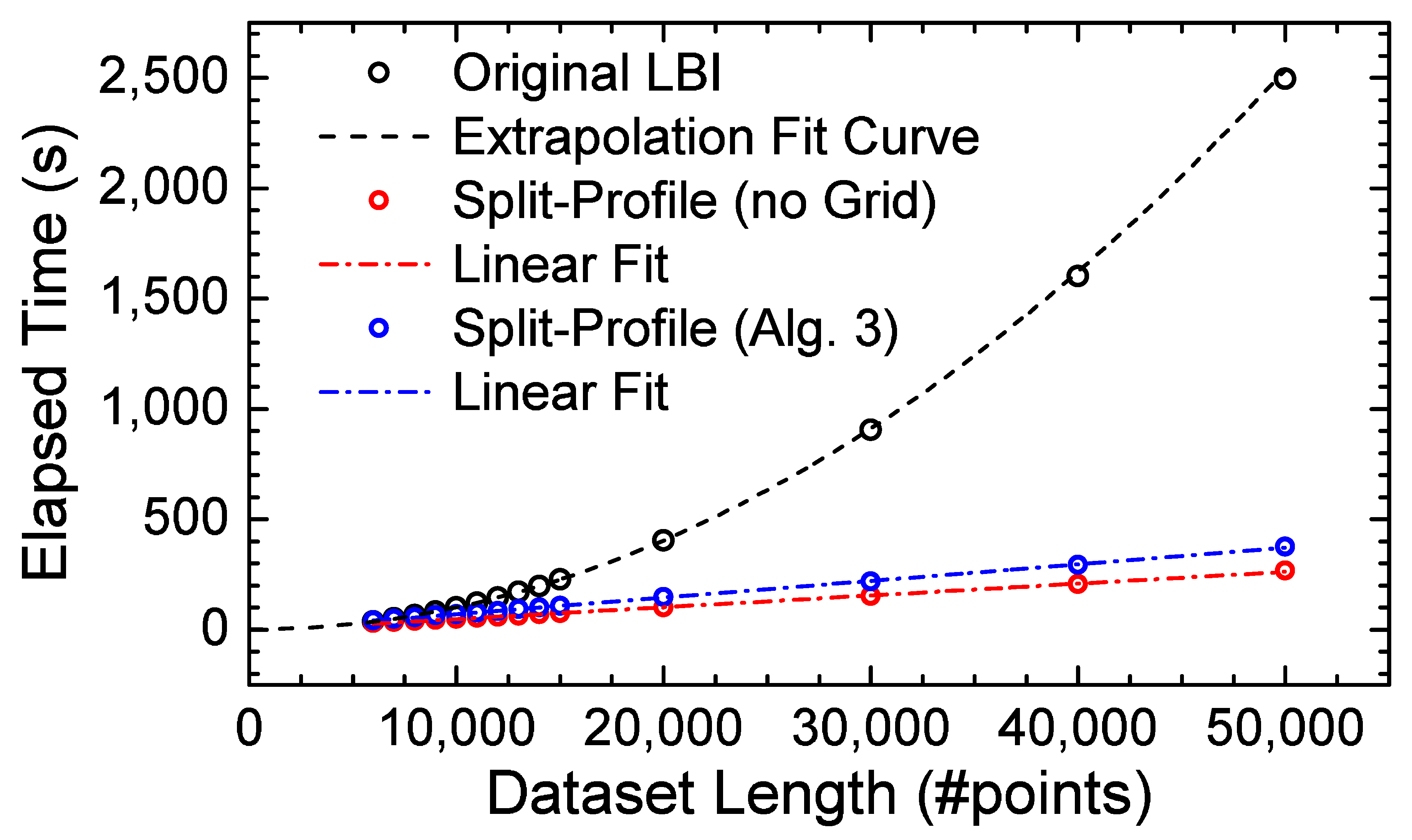
The choice of the split-profile length was, in contrast with the $\lambda$ selection, a much less meaningful parameter of the split-profile methodology. However, it remained as a free parameter of this methodology and had to undergo scrutiny as well. As observed in Figure 4, the split-profile length imposed a minimum threshold that, if respected, maintained the quality of the results. There, the performance results for different split-profile lengths are depicted in terms of: the relative false positive and true positive incidence, as well as the MCC. For these results, 1000 datasets, each 15,000 points long, were sorted and constructed using Algorithm 2 and later analyzed with the split-profile LBI—Algorithm 3—using different split-profile lengths. At the same time, the same datasets were analyzed with the original (non-split) LBI algorithm, to serve as a control group; the results of this analysis represent the baselines—or the thresholds to be met—in the panels of Figure 4.

This effect had quite a discernible origin, since reducing the instance size analyzed by any sparse technique reduced its signal denoising capabilities. In summary, the results indicated that the minimum split-profile length that allowed the original performance to be met was ∼4500. Below this value, the split-profile LBI produced an overflow of false positives, and the MCC dropped significantly. As the length increased, however, the total time necessary for the algorithm to elapse also increased; therefore, the chosen operational value was set as the minimum such that the original performance was met. The choice of 4500 for the results of Figure 3 followed from this analysis.

3.3. Timing Results

The parameters and procedures that allowed the split-profile LBI to uphold the performance level set by the original LBI algorithm when applied to trend break detection in optical fiber profiles was determined with a thorough analysis in the previous section. These were the $\lambda$ selection and scaling, the initial value of $\lambda =0.5$ in the grid, and the split-profile length of ∼4500 points.

Finally, then, it was left to determine the impact of the split-profile methodology on the elapsed time of the algorithm, which was the driving motivation behind its development. For this analysis, the results of Figure 2 were used as a reference. Furthermore, two different timing curves are presented in Figure 5: the full processing time of Algorithm 3, including the extra necessary iterations to perform the $\lambda$-grid selection; and the processing time without the grid, i.e., in case the algorithm was to be halted before Line 7 of Algorithm 3. This result was important to showcase the minimum relative impact that the extra iterations required by the grid had on the total processing time in contrast with the impact that they had on the overall performance of the split-profile LBI, as shown in Figure 3.

By adjusting the length and the selection of $\lambda$, the performance of the split-profile LBI was upheld, and simultaneously, a dramatic decrease in the total processing time was observed. In fact, as the results of Figure 5 showed, once the length was fixed, the time scaled linearly with the length of the dataset being processed instead of quadratically: as the split length was fixed, the overall processing time was comprised of the time required for processing one split-profile multiplied by the number of total splits plus a processing overhead. The results of the original LBI algorithm are reproduced from Figure 2—in black along with its parabolic fit—for reference. The results of the complete split-profile LBI—Algorithm 3—are shown in blue, which represent a minor increase with respect to those in red, which correspond to not performing the $\lambda$-grid. For both these results, a linear fit was used, with an associated $R^2$ value of $0.999$ and $0.998$ when considering and not considering the grid, respectively. As in the analysis of the timing of the original LBI, the linear fit was performed, for the split-profile LBI, only within the first points, in the range $\left[6000:\mathrm{15,000}\right]$, and then extrapolated to the other points, showing that the fit was indeed consistent as the length of the dataset increased.

4. Discussion: Parallelization of Profile-Split in Dedicated Hardware

The results of Figure 5, even though quite striking, were acquired after running the algorithm on a workstation $\mathrm{I}\mathrm{NTEL} \mathrm{X}\mathrm{EON} \mathrm{CPU} E5-2690 V4$ at 2.6 GHz and 512 GB RAM). As set forth in [12], however, the core of the LBI algorithm could benefit immensely from hardware-dedicated implementation. There, individual Block RAMs (BRAMs) were structured such that data from each iteration could be fed in parallel to an arithmetical unit, greatly expediting the procedure. In fact, the total number of clock cycles necessary for the algorithm to elapse given the total number of iterations and the amount of available memory structures (BRAMs) in such a dedicated hardware was analytically determined and confirmed for commercial FPGAs [12] and was as follows:

$$\begin{array}{c}C\left(N,M,\alpha ,F\right)=\hfill \\ F+\sum _{i=1}^L\left[3\left(⌈\frac{\left(\left(i-1\right)\%N\right)+1}{M}⌉+2\right)+\lceil {log}_{2}M\rceil \right],\hfill \end{array}$$

(6)

where the operator $\lceil ·\rceil$ denotes the ceiling operation, N is the instance size, L is the total number of iterations ($L=\alpha N$, M is the number of available BRAMS, and F is an (overall negligible) offset associated with initialization and control instructions ($F=22$) [12]. By associating this value with the maximum achievable clock frequency in the target FPGA, the processing time could be determined, i.e.,

$$T_{\mathrm{proc}}=\frac{C(N,M,\alpha ,F)}{f_{\max }}.$$

(7)

In a profile-split scenario, pre-determined stretches of data of fixed size (N∼4500 according to Section 3) were processed individually. The free-parameters of Equation (6) were, thus, reduced to $\alpha$, M, and $f_{\max }$. The first, albeit a choice of the operator, was shown to yield highly accurate results at values $\alpha =450$ or greater [12] and could also be fixed. The latter two were limited by the availability of resources on the FPGA chip and the optimality of the clock distribution inside the chip. In order, thus, to expand the analysis, two target FPGA chips, namely Altera’s C$\mathrm{YCLONE}$ V and S$\mathrm{TRATIX}$ V, were selected as potential platforms for the implementation of the parallel split-profile LBI. Making use of the hardware design established in [12] for an FPGA-embedded LBI unit, the resource usage and maximum estimated clock frequency for different unit sizes were determined and are presented in Figure 6. Here, the unit size was determined by the number of BRAMs included in the design.

Simple linear regressions applied to each of the datasets—also depicted in Figure 6—enabled one to estimate, given the number of BRAMs in the design, both the resource usage and the maximum clock frequency for the target FPGAs. Based on these, operation conditions for different hardware options could be determined. Here, three such options were considered: the original LBI hardware, consisting of a single unit that utilized the chip’s full resource capacity and processed the whole dataset without splitting; a sequential split-profile implementation, where a single unit making use of the chip’s full resource capacity processed individual sub-profiles one after the other; and the simultaneous split-profile implementation, where multiple units, each making use of a portion of the chip’s full resource capacity, processed individual sub-profiles at the same time.

The objective of the comparative analysis between the three options was to gauge: the speed-up level of the split-profile methodology as opposed to the original LBI in a hardware scenario; the minimum processing time achieved by the split-profile LBI; and finally, the tradeoff between simultaneous processing and full resource utilization. In order to perform the analysis correctly, whose results are depicted in Figure 7, the following practical observations are due:

• The analysis was restricted to the S$\mathrm{TRATIX}$ V, since the C$\mathrm{YCLONE}$ V did not offer enough resources for a fruitful analysis for a large range of profile lengths.
• Due to the fact that the difference in processing times between the split-profile and the original LBI was insignificant for datasets containing fewer than 20,000 points—according to the analysis of Figure 5—this was set as the starting point of the analysis.
• The goal was to observe the trend of the total processing time curve for the three hardware options (original LBI, sequential split, simultaneous split) as the dataset length increased. Therefore, up to ${10}^7$ points were considered for the analysis.
• Due to the data storage architecture and assuming a 20 bit long word BRAM with 1024 positions, each BRAM had a data capacity of 333 points [12].
• The BRAM storage capacity could be combined with the stipulated size of the profile-split ($N_{\mathrm{split}}=4480$) in order to determine the minimum number of BRAMs assigned to each unit (14).
• The curve that associated the resource usage in the FPGA to the number of instantiated BRAMs (Figure 6) could be used to determine the maximum number of individual split-profile units that could be simultaneously instantiated in the S$\mathrm{TRATIX}$ V (38, with 98.08% resource usage) and, in turn, the maximum number of data points that could be stored ($38·4480=$ 170,240, highlighted in Figure 7).
• The curve that associated the resource usage in the S$\mathrm{TRATIX}$ V to the number of instantiated BRAMs (Figure 6) could be used to determine the maximum number of BRAMs that could be used for the original LBI implementation (1392, with 99.06% resource usage) and, in turn, the maximum number of data points that could be stored in the FPGA ($333\times 1392$ = 463,536, highlighted in Figure 7).
• If the dataset to be processed was longer than the maximum storage capacity of the hardware, full processing would not be possible in a single step, requiring the data points to be processed in batches.
• Processing data in batches required extra time necessary for loading/unloading of data to be taken into account. According to [12], this procedure took one clock cycle per data point and, although negligible, was included for completeness.
• Provided the sub-profile segmentation was respected through batch processing, no further care was needed in a profile-split scenario.
• In the original LBI implementation, batch processing required an additional $\lambda$ selection step (as was necessary in the split-profile case), otherwise the performance would decrease drastically. The procedure described in Section 3 could be employed such that the original performance was maintained.

The most straightforward observation that could be made from Figure 7 is that the simultaneous split-profile, which made use of multiple units of the split-profile LBI instantiated in the same hardware, outperformed the other solutions. The sequential split-profile hardware, when implemented in the S$\mathrm{TRATIX}$ V, exhibited a ∼3-fold asymptotic time increase with respect to the simultaneous split-profile hardware, still figuring as an excellent candidate for implementation in smaller FPGA chips (such as the C$\mathrm{YCLONE}$ V), where instantiating a single unit was beneficial. Furthermore, since the software version of the split-profile LBI used to extract the results of Figure 5 also performed sequential processing of the sub-profiles, the timing comparison between this and the sequential hardware could be made on the same grounds: while the software version required close to 300 s to process a 50,000 point long dataset, the sequential hardware elapsed in about 1.1 s, a close to 300-fold reduction.

Quite noticeable as well in Figure 7 are the discrete jumps taken by the black (original LBI) and blue (simultaneous split LBI) curves. As commented before, in case the dataset contained more points than could be stored by a particular hardware, batch processing was required. Whenever the number of necessary batches increased, the lines performed a jump. Above the marked value of 170,240, for instance, the blue curve jumps since the number of necessary batches is two; it then remains stationary since, even though the dataset length is increasing, only two batches are necessary. When the dataset is long enough such that three batches are necessary, it jumps again, and so forth.

The above described behavior is also observed in the black curve, although for this curve, a slope break is also observed, which must be discussed. For small dataset lengths, the original LBI processed the data without batches and, therefore, followed the quadratic complexity curve that was already been discussed in Section 2 and Figure 5. The fact that the slope of the timing curve in LOG-LOG scale was close to two was a consequence of its quadratic behavior. When the dataset increased such that batch-processing became necessary (above the marked value of 463,536), the batching had the effect of splitting the original profile into smaller sub-profiles, thus artificially inducing a split-profile character. In the asymptotic regime, the slope then acquired the characteristics of the split-profile curves (blue and red) with a LOG-LOG slope close to one, indicating a linear increase of the total processing time.

5. Materials and Methods

To evaluate the capabilities of the proposed architecture, the following methods were used: a commercially available state-of-the-art synthesis software (Intel Quartus Prime) was used to evaluate the maximum clock frequency and the device occupation of the design for different sizes (i.e., the number of used block RAMs in parallel).

6. Conclusions

The profile-split methodology ensured comparable algorithm performance while overcoming the quadratic scaling of the elapsed time, which became a severe hindrance for long instance sizes. As it stands, no information from any of the splits was necessary so that another split could be processed, and thus, simultaneous processing of each of the split profiles was a possibility. The results from Section 3 stipulated optimized parameters for individual hardware units implementing Algorithm 3, in particular with respect to the size, or number of data points, assigned to each of these units. This, in turn, enabled an analysis, in Section 4, of the impact of implementing multiple units that simultaneously processed data inside an embedded unit, such as an FPGA, with limited resources in terms of memory and logical elements. The limited resources created a constraint on the number of total parallel units that could be instantiated and put the advantages of this methodology to a more stringent test. The processing times of a few seconds for datasets as long as 100,000 points associated with an MCC value of 0.84 placed the hardware-embedded split-profile linearized Bregman iterations algorithm as the candidate of choice for trend break detection problems.

References

1. Yin, W.; Osher, S.; Goldfarb, D.; Darbon, J. Bregman iterative algorithms for _1-minimization with applications to compressed sensing. SIAM J. Imaging Sci. 2008, 1, 143–168. [Google Scholar] [CrossRef] [Green Version]
2. Cai, J.F.; Osher, S.; Shen, Z. Linearized Bregman iterations for compressed sensing. Math. Comput. 2009, 78, 1515–1536. [Google Scholar] [CrossRef]
3. Cai, J.F.; Osher, S.; Shen, Z. Linearized Bregman iterations for frame-based image deblurring. SIAM J. Imaging Sci. 2009, 2, 226–252. [Google Scholar] [CrossRef]
4. Osher, S.; Mao, Y.; Dong, B.; Yin, W. Fast linearized Bregman iteration for compressive sensing and sparse denoising. Commun. Math. Sci. 2010, 8, 93–111. [Google Scholar]
5. Goldstein, T.; Osher, S. The split Bregman method for L1-regularized problems. SIAM J. Imaging Sci. 2009, 2, 323–343. [Google Scholar] [CrossRef]
6. Choi, K.; Fahimian, B.P.; Li, T.; Suh, T.S.; Lei, X. Enhancement of four-dimensional cone-beam computed tomography by compressed sensing with Bregman iteration. J. X-ray Sci. Technol. 2013, 21, 177–192. [Google Scholar] [CrossRef]
7. Lorenz, D.A.; Wenger, S.; Schöpfer, F.; Magnor, M. A sparse Kaczmarz solver and a linearized Bregman method for online compressed sensing. In Proceedings of the 2014 IEEE International Conference on Image Processing (ICIP), Paris, France, 27–30 October 2014; pp. 1347–1351. [Google Scholar]
8. Lunglmayr, M.; Huemer, M. Efficient linearized Bregman iteration for sparse adaptive filters and Kaczmarz solvers. In Proceedings of the 2016 IEEE Sensor Array and Multichannel Signal Processing Workshop (SAM), Rio de Janerio, Brazil, 10–13 July2016; pp. 1–5. [Google Scholar]
9. Riley, W.J. Algorithms for frequency jump detection. Metrologia 2008, 45, S154–S161. [Google Scholar] [CrossRef]
10. Babcock, H.P.; Moffitt, J.R.; Cao, Y.; Zhuang, X. Fast compressed sensing analysis for super-resolution imaging using L1-homotopy. Opt. Express 2013, 21, 28583–28596. [Google Scholar] [CrossRef] [Green Version]
11. Lunglmayr, M.; Amaral, G.C. Linearized Bregman Iterations for Automatic Optical Fiber Fault Analysis. IEEE Trans. Instrum. Meas. 2018, 68, 3699–3711. [Google Scholar] [CrossRef]
12. Calliari, F.; Amaral, G.C.; Lunglmayr, M. FPGA-Embedded Linearized Bregman Iterations Algorithm for Trend Break Detection. arXiv 2019, arXiv:1902.06003. [Google Scholar]
13. Amaral, G.C.; Garcia, J.D.; Herrera, L.E.; Temporao, G.P.; Urban, P.J.; von der Weid, J.P. Automatic fault detection in wdm-pon with tunable photon counting otdr. J. Light. Technol. 2015, 33, 5025–5031. [Google Scholar] [CrossRef]
14. Von der Weid, J.P.; Souto, M.H.; Garcia, J.D.; Amaral, G.C. Adaptive filter for automatic identification of multiple faults in a noisy otdr profile. J. Light. Technol. 2016, 34, 3418–3424. [Google Scholar] [CrossRef] [Green Version]
15. Urban, P.J.; Vall-Llosera, G.; Medeiros, E.; Dahlfort, S. Fiber plant manager: An OTDR-and OTM-based PON monitoring system. IEEE Commun. Mag. 2013, 51, S9–S15. [Google Scholar] [CrossRef]
16. Hornsteiner, A. Fiber Optic Technology Trends in Data Transmission: Digitalization of data advance the need for constant upgrading of data networks. Opt. Photonik 2017, 12, 20–24. [Google Scholar] [CrossRef] [Green Version]
17. Candès, E.; Romberg, J.; Tao, T. Robust uncertainty principles: Exact signal reconstruction from highly incomplete frequency information. IEEE Trans. Inf. Theory 2006, 52, 489–509. [Google Scholar] [CrossRef] [Green Version]
18. Han, P.Z.; Li, P.H.; Yin, P.W. Compressive Sensing for Wireless Networks; Cambridge University Press: Cambridge, MA, USA, 2013. [Google Scholar]
19. Calliari, F.; Herrera, L.E.; von der Weid, J.P.; Amaral, G.C. High-dynamic and high-resolution automatic photon counting OTDR for optical fiber network monitoring. In Proceedings of the 6th International Conference on Photonics, Optics and Laser Technology, Funchal, Portugal, 25–27 January 2018; Volume 1, pp. 82–90. [Google Scholar]
20. Bühlmann, P.; Rütimann, P.; van de Geer, S.; Zhang, C.H. Correlated variables in regression: Clustering and sparse estimation. J. Stat. Plan. Inference 2013, 143, 1835–1858. [Google Scholar] [CrossRef] [Green Version]
21. Bertsimas, D.; King, A.; Mazumder, R. Best subset selection via a modern optimization lens. Ann. Stat. 2016, 44, 813–852. [Google Scholar] [CrossRef] [Green Version]
22. Saavedra, R.; Tovar, P.; Amaral, G.C.; Fanzeres, B. Full Optical Fiber Link Characterization With the BSS-Lasso. IEEE Trans. Instrum. Meas. 2018, 68, 4162–4174. [Google Scholar] [CrossRef] [Green Version]
23. Barnoski, M.; Rourke, M.; Jensen, S.; Melville, R. Optical time domain reflectometer. Appl. Opt. 1977, 16, 2375–2379. [Google Scholar] [CrossRef]
24. Amaral, G.C.; Herrera, L.E.; Vitoreti, D.; Temporão, G.P.; Urban, P.J.; der von Weid, J.P. WDM-PON monitoring with tunable photon counting OTDR. IEEE Photonics Technol. Lett. 2014, 26, 1279–1282. [Google Scholar] [CrossRef]
25. Schwarz, G. Estimating the dimension of a model. Ann. Stat. 1978, 6, 461–464. [Google Scholar] [CrossRef]
Figure 1. Effect of the inclusion of the slope component in the analysis of a fiber profile. In the upper panel, the original OTDR dataset containing the slope component is depicted. In the lower panel, two different LBI fault detection results are presented; when the slope is not included, a high incidence of false positives can be distinguished, which vanishes when the slope is considered.
Electronics 09 00423 g001
Figure 2. Elapsed times of the LBI algorithm for different dataset lengths. Following the complexity analysis of the algorithm, a parabolic curve is fitted to the first ten points of the curve (6000 to 15,000 points, marked in blue) and further extrapolated to the higher values. As can be seen, the curves fall exactly into the extrapolated curve, confirming the complexity analysis.
Electronics 09 00423 g002
Figure 3. Performance comparison between three different versions of the analysis algorithm. Even though the differences of TPs and TFs might not seem extremely drastic for the split-profile simple, the broader characterization enabled by the MCC makes it clear that there is a deep performance drop if λ is not correctly chosen.
Electronics 09 00423 g003
Figure 4. Performance of the split-profile methodology for varying split-profile lengths, in number of points. The original profiles, from which the sub-profiles were derived, contained 15,000 points. To increase the statistical validity of the analysis, 1000 datasets were generated according to Algorithm 2. The baselines—in black dashes—correspond to the results of the original (non-split) LBI. Above 4500 points, the performance recovered and slightly increased even when the λ -grid (Lines 7 through 10 in Algorithm 3) was not performed, as evidenced by a higher MCC value.
Electronics 09 00423 g004
Figure 5. Final timing comparison between the original LBI and the corresponding split-profile LBI; two versions of the latter, with and without the λ -grid, are depicted. For shorter dataset lengths, the effect of the split-profile methodology is rather negligible since the original length is comparable to the individual split-profile length; however, as the dataset length increases above 20,000 points, a very clear distinction can be observed between the total elapsed times of the variants of the analysis algorithm.
Electronics 09 00423 g005
Figure 6. Resource and timing analysis for two FPGA chips of different sizes: the smaller C YCLONE V; and the mid-range S TRATIX V. These results correspond to the optimal place-and-route procedure of commercially available hardware-design software, namely the Q UARTUS P RIME software.
Electronics 09 00423 g006
Figure 7. Total processing time as a function of the dataset length for three possible hardware implementations in the S TRATIX V. The results are displayed in LOG-LOG scale for ease of visualization. Striking features, discussed in the text, are: the slope break of the original LBI curve, which corresponds to the transition to batch processing; the equivalence between the asymptotic slopes of all three curves; and the dominance of the simultaneous split-profile hardware in terms of processing time over the other options.
Electronics 09 00423 g007