Resource Allocation with a Rate Guarantee Constraint in Device-to-Device Underlaid Cellular Networks

Abstract

Device-to-device (D2D) communication is a crucial technique for various proximity services. In addition to high-rate transmission and high spectral efficiency, a minimum data rate is increasingly required in various applications, such as gaming and real-time audio/video transmission. In this paper, we consider D2D underlaid cellular networks and aim to minimize the total channel bandwidth while every user equipment (UE) needs to achieve a pre-determined target data rate. The optimization problem is jointly involved with matching a cellular UE (CU) to a D2D UE (DU), and with channel assignment and power control. The optimization problem is decoupled into two suboptimization problems to solve power control and channel assignment problems separately. For arbitrary matching of CU, DU, and channel, the minimum channel bandwidth of the shared channel is derived based on signal-to-interference-plus-noise ratio (SINR)-based power control. The channel assignment is a three-dimensional (3-D) integer programming problem (IPP) with a triple (CU, DU, channel). We apply Lagrangian relaxation, and then decompose the 3-D IPP into two two-dimensional (2-D) linear programming problems (LPPs). From intensive numerical results, the proposed resource allocation scheme outperforms the random selection and greedy schemes in terms of average channel bandwidth. We investigate the impact of various parameters, such as maximum D2D distance and the number of channels.

1. Introduction

The fifth-generation (5G) network is expected to create new services in diverse industries [1]. One of the newly enabled services in 5G is proximity service in the vehicle-to-everything (V2X) network, the public safety network, and the social network, etc. Recently, there has been an increasing demand for services that require high data rates and low latency [2]. For example, in V2X communications, lane merge, see-through, and remote driving for parking are representative use cases [3]. In public safety networks, mission-critical tasks in an emergency, and remote monitoring through voice/video transmission require data rates of over 1 Mbps and low latency [4,5].

Device-to-device (D2D) communication has been recognized as a crucial technology to support proximity services in 5G [1,6], since it enables devices in the same vicinity to communicate directly with each other without routing the data paths through a network infrastructure. Herein, D2D user equipment (DU) consists of a D2D transmitter (DT) and a D2D receiver (DR). As direct communication between devices is possible, D2D communication is advantageous in terms of latency, compared to traditional communications via network infrastructure, e.g., the Uu-interface in the 3rd Generation Partnership Project (3GPP). In addition, because the distance between devices is relatively shorter than the distance between a device and its corresponding base station (BS), better link quality can be acquired in D2D communications, which is advantageous in terms of high-rate transmissions and reliability. Furthermore, in D2D underlaid networks where DUs share spectrum with cellular user equipments (CUs), spectrum efficiency and network capacity can be further improved [7].

However, in D2D underlaid cellular networks, there is a possibility of severe interference due to resource sharing between CUs and DUs. Therefore, interference management must be applied to effectively handle the interference, and to guarantee a certain degree of quality of service (QoS). In the literature, various power control and resource allocation schemes have been proposed to guarantee QoS requirements in terms of signal-to-interference-plus-noise ratio (SINR) or minimum required data rate [8,9,10,11,12,13,14,15,16,17]. In [8], a power control scheme was studied to maximize the sum of the achievable data rates of a CU–DU pair. However, only the SINR of the CU is guaranteed to be greater than or equal to a pre-determined SINR threshold. In [9], multiple DUs can be matched to a single CU and an optimal energy-efficient power control scheme was proposed while guaranteeing the minimum required data rate of each user equipment (UE). However, only a single channel was taken into account and, hence, the resource allocation or channel assignment problem was not addressed. In [10], a resource allocation scheme was studied while assuming that the transmit power of UEs is fixed. Joint power control and resource allocation schemes were proposed in [11,12,13,14,15,16,17]. A single DU is assigned to only one channel, and vice versa in [11,12], whereas multiple DUs are allowed to be assigned to the same channel in [13,14]. In addition, a DU is allowed to be assigned to multiple channels in [15,16,17]. In addition to power control and resource allocation, mode selection for DUs and relay selections were considered in [18,19,20] and [21,22], respectively. In the above-mentioned studies, a fixed channel bandwidth is allocated to each channel and moreover, a channel is pre-assigned to a CU in advance, and hence, the remaining channel assignment problem is to choose the best DU for each CU.

In most previous sum rate or energy efficiency maximization schemes [8,9,10,11,12,13,14,15,16,17,18,19,20,21,22], even though SINR or minimum data rate per UE was considered as a constraint, the individual data rate may not be guaranteed with a fixed amount of channel bandwidth. When the received SINR is low due to high interference and maximum transmit power limitation, the fixed channel bandwidth may not be wide enough to guarantee the target rate. In D2D underlaid cellular networks, UEs experience diverse interference situations depending on CU–DU matching and power control, so the fixed channel bandwidth assumption may not be beneficial. In mobile communication systems, a proper modulation and coding scheme (MCS) needs to be informed during a scheduling process for successful reception [23,24]. It is also noted that resource information indicating the amount of resource and its location can be informed and, therefore, the channel bandwidth can be adaptively adjusted. Thus, it is optimal to manage the transmit power, channel bandwidth, and channel assignment jointly. However, to the best of our knowledge, there is no research on the resource allocation problem with rate guarantee constraints where the total channel bandwidth is minimized while ensuring that all the UEs can achieve their target data rates.

The contributions of this paper are as follows:

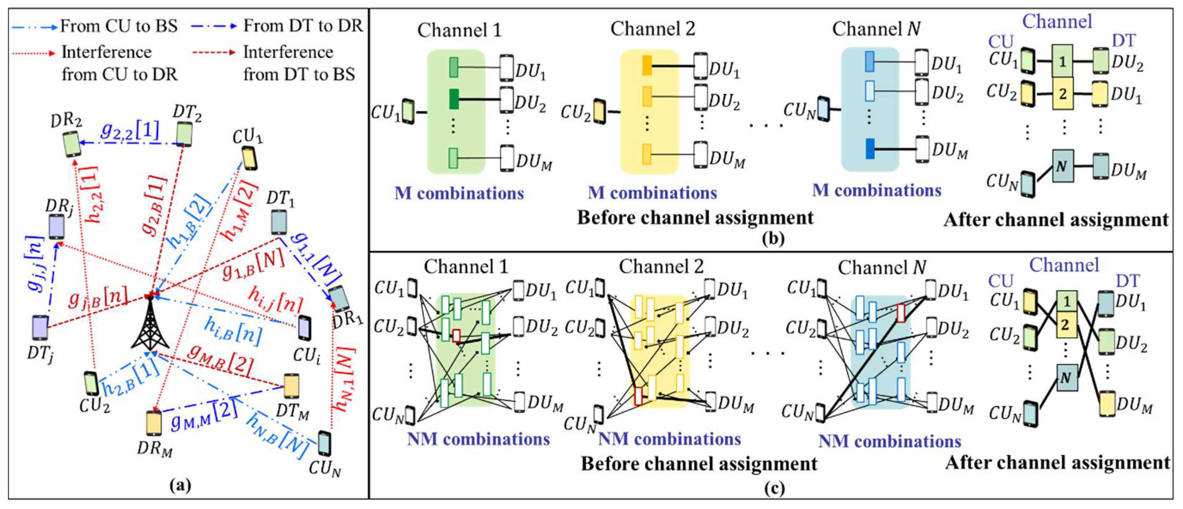
• In most previous studies, each CU was assumed to have a preassigned channel, and thus, the channel assignment problem is to find the best DU for each CU in order to maximize the sum rate or energy efficiency. Then, the assigned channel information needs to be informed to the corresponding DUs. However, as indicated in [23,24], the channel information can be informed to CUs as well as DUs and, therefore, the channels can be re-assigned for CUs. Now, the channel assignment problem becomes the triple matching problem with pairs of (CU, DU, channel). This three-dimensional (3-D) channel assignment increases the possibility of choosing a better channel and can bring a performance improvement at the cost of increased computational complexity. To mitigate that extra complexity, a suboptimal algorithm is proposed by using Lagrangian relaxation and a sub-gradient-based iterative algorithm;
• We consider a system where the channel bandwidth is not fixed but is adaptively determined based on the triple (CU, DU, channel). As the received SINR varies, the channel capacity changes and, therefore, the channel bandwidth required to guarantee the target data rate needs to be adjusted. In more detail, the minimum channel bandwidth to guarantee the target data rate is derived with a maximum transmit power constraint. Each CU–DU–channel match-up requires different minimum channel bandwidths. In addition, hence, the remaining problem is a 3-D assignment problem to minimize the overall channel bandwidth, while guaranteeing the target data rate;
• Since the channel is shared, increasing the transmit power of CU may cause severe interference to DU and vice versa. In this paper, the exact solution to the power control problem involves iterative calculations through, for example, a root-finding algorithm. To reduce complexity, a suboptimal algorithm is proposed where power can be calculated in a closed form. In previous works, the transmit power of the UEs is determined with a fixed channel bandwidth. Even though SINR or minimum data rate per UE is considered as a constraint, some UEs may not meet the constraint, i.e., the feasible set becomes empty due to maximum transmit power limitation and fixed channel bandwidth. Herein, the channel bandwidth can be adaptively determined according to the received SINR to meet the minimum data rate.

2. System Model and Problem Formulation

2.1. System Model

Figure 1a illustrates a D2D underlaid cellular network where the uplink channel is shared. We consider a single cell where $N$ cellular UEs (CUs) and $M$ $\left(N\ge M\right)$ D2D transmitters (DTs) are randomly positioned in the cell. A DT and one D2D receiver (DR) form a D2D UE (DU), and a DR is uniformly distributed within a circle whose origin is at its corresponding DT with a radius of $D_{max}^d$. We assume that every CU and DT are equipped with a single transmit antenna. The BS and every DR are equipped with a single receive antenna. The network is assumed to be provided with $N$ orthogonal channels on which channel bandwidths are variable. Every UE is assigned only one channel. Moreover, every channel is either allocated to one CU alone or to a match-up of one CU and one DU for sharing. Every DU should be matched with a CU to share a channel for transmission. If channel $n$ is shared by CU $i$ ($C{U}_i$) and DU $j$ ($D{U}_j$), $C{U}_i$ and $D{T}_j$ transmit signals to the BS and to DR $j$ ($D{R}_j$), respectively, at the same time. Here, to denote the channel gain of the links from the CUs, we use the letter $h$. Furthermore, for the index of the BS, we use $B$. Then, the channel gain of the link from $C{U}_i$ to the BS on channel $n$ is denoted as $h_{i,B}\left[n\right]$. We use the letter $g$ to denote the channel gain for the links from the DTs, e.g., $g_{j,j}\left[n\right]$ denotes the channel gain of the link from $D{T}_j$ to $D{R}_j$ on channel $n$. Note that the signal from $D{T}_j$ to $D{R}_j$ causes co-channel interference (CCI) with the BS, and the corresponding channel gain is denoted as $g_{j,B}\left[n\right]$. Similarly, $h_{i,j}\left[n\right]$ denotes the channel gain of the link from $C{U}_i$ to $D{R}_j$. The channel state information (CSI) of the links can be acquired by utilizing either a sounding reference signal (SRS) or reference signal (RS) associated with THE D2D link [25,26]. In this paper, we assume that the CSI of all possible combinations of the links is available at the BS, which may require indispensable CSI feedback. However, this assumption has been widely used in previous literature for performance evaluation [7,8,9,11,12,13,14,15,16,17,18,19].

Figure 1b illustrates a channel assignment scheme, where each channel with a fixed channel bandwidth is pre-assigned to one CU before the channel assignment. In each channel, there exist $M$ boxes where their size implies the channel bandwidth, and the intensity of the box color represents the sum rate of the corresponding match-up of CU and DU. For instance, channel $1$ is pre-assigned to $C{U}_1$, and the color intensity varies depending on which DU is matched to share channel 1. For channel 1, the match-up of $C{U}_1$ and $D{U}_2$ is the best one from among $M$ possible matches, and thus, the corresponding box linked to $D{U}_2$ is painted with the darkest green color. Similarly, $D{U}_1$ and $D{U}_M$ are selected as the best matches for $C{U}_2$ and $C{U}_N$, respectively. On the rightmost side in Figure 1b, the result of the channel assignment is shown.

Meanwhile, Figure 1c illustrates the 3-D channel assignment scheme proposed in this paper. The channel bandwidth, which corresponds to the size of each box, is determined adaptively based on the channel capacity of each match-up so the CU and DU can achieve the pre-determined target data rate. Note that if a channel is shared, depending on which CU and DU are matched, the CCI and, accordingly, the channel capacity can vary on a case-by-case basis. Therefore, on each channel, there exist $NM$ possible matches with different bandwidths, which are illustrated by $NM$ different boxes in Figure 1c. When the channel is assigned to minimize the sum bandwidth, the best match per channel is decided based on the channel bandwidth. For instance, matching $C{U}_2$ and $D{U}_2$ corresponds to the smallest box on channel 1 and can be the best match on channel 1. Similarly, $C{U}_1$ and $D{U}_M$ can be the best match on channel 2, and $C{U}_N$ and $D{U}_1$ can be the best match on channel $N$. The rightmost side in Figure 1c shows the result of the channel assignment where the channel bandwidths are different. Here, we need to note that the DU chosen as the best match in an earlier selection phase can be the best match for a later selection phase as well. For example, $D{U}_M$ can also be the best match for $C{U}_3$. So, to find the best channel assignment involves searching for a total of $N^{2}M$ possible matches.

2.2. Problem Formulation

Now, let us calculate the minimum required channel bandwidth, $b_{i,j}\left[n\right]$, for an arbitrary match-up of $C{U}_i$ and $D{U}_j$ on channel n to guarantee the target data rate. For simplicity, the target data rates of the CU and DU are denoted as $R_T^c$ and $R_T^d$, respectively. $C{U}_i$ transmits signals with power $P_i^c$ to the BS, and $D{T}_j$ transmits signals with power $P_j^d$ to $D{R}_j$. Then, given the channel bandwidth for $C{U}_i,b_{i,j}^c\left[n\right]$, SINR at the BS can be expressed as

$${\gamma }_{i,j}^c\left[n\right]=\frac{P_i^c{h}_{i,B}\left[n\right]}{P_j^d{g}_{j,B}\left[n\right]+b_{i,j}^c\left[n\right]{\sigma }_0^2},$$

(1)

where ${\sigma }_0^2$ is the noise power density. Then, the achievable data rate, $R_{i,j}^c\left[n\right]$, needs to guarantee $R_T^c$:

$$R_{i,j}^c\left[n\right]\triangleq b_{i,j}^c\left[n\right]{\log }_2\left(1+{\gamma }_{i,j}^c\left[n\right]\right)\ge R_T^c.$$

(2)

Similarly, with the channel bandwidth for $D{T}_j,b_{i,j}^d\left[n\right]$, the SINR at $D{R}_j$ can be written as

$${\gamma }_{i,j}^d\left[n\right]=\frac{P_j^d{g}_{j,j}\left[n\right]}{P_i^c{h}_{i,j}\left[n\right]+b_{i,j}^d\left[n\right]{\sigma }_0^2}$$

(3)

and the following condition needs to be satisfied:

$$R_{i,j}^d\left[n\right]\triangleq b_{i,j}^d\left[n\right]{\log }_2\left(1+{\gamma }_{i,j}^d\left[n\right]\right)\ge R_T^d$$

(4)

Then, to guarantee both $R_T^c$ and $R_T^d$ concurrently, $b_{i,j}\left[n\right]$ should be determined as follows:

$$b_{i,j}\left[n\right]\ge \max \left(b_{i,j}^c\left[n\right],b_{i,j}^d\left[n\right]\right)$$

(5)

We assigned the channels to minimize the total channel bandwidth, while guaranteeing $R_T^c$ and $R_T^d$ for the CUs and DUs, respectively. To minimize the total channel bandwidth, a total of $N^{2}M$ possible matches need to be investigated. In addition, the transmission power of the CUs and the DTs should be optimally determined. Here, we introduce ${\Omega }_c=\left\{1,\dots ,N\right\}$ and ${\Omega }_d=\left\{1,\dots ,M\right\}$ to denote the sets of CUs and DUs, respectively. Moreover, we introduce a channel matching indicator: $x_{i,j}\left[n\right]$. When $C{U}_i$ and $D{U}_j$ share a channel $n$, $x_{i,j}\left[n\right]$ is set at 1; it is 0 otherwise:

$$x_{i,j}\left[n\right]=\{\begin{array}{c}1,\mathrm{if}C{U}_i\mathrm{and}D{U}_j\mathrm{share}\mathrm{channel}n\hfill \\ 0,\mathrm{otherwise}\hfill \end{array}$$

(6)

For simplicity, we assume that $N=M$, i.e., the number of CUs is the same as that of DUs. When $N>M$, $\left(N-M\right)$ CUs have no match. Although the CUs that are not matched also creates a resource allocation problem, it is trivial and straightforward. Then, the proposed optimization problem that minimizes the overall bandwidth can be formulated as follows:

$$\mathbf{𝒫}\mathbf{1}:\underset{P_i^c,P_j^d,x_{i,j}\left[n\right]}{\min }{\displaystyle \sum }_{i\in {\Omega }_c}{\displaystyle \sum }_{j\in {\Omega }_d}{\displaystyle \sum }_{n=1}^N{x}_{i,j}\left[n\right]b_{i,j}\left[n\right]$$

(7)

subject to

$${\displaystyle \sum }_{j\in {\Omega }_d}{\displaystyle \sum }_{n=1}^N{x}_{i,j}\left[n\right]=1,\forall i\in {\mathsf{\Omega }}_c$$

(7a)

$${\displaystyle \sum }_{i\in {\Omega }_c}{\displaystyle \sum }_{n=1}^N{x}_{i,j}\left[n\right]=1,\forall j\in {\Omega }_d$$

(7b)

$${\displaystyle \sum }_{i\in {\Omega }_c}{\displaystyle \sum }_{j\in {\Omega }_d}{x}_{i,j}\left[n\right]\le 1,\forall n=1,\dots ,N$$

(7c)

$${\displaystyle \sum }_{j\in {\Omega }_d}{\displaystyle \sum }_{n=1}^N{x}_{i,j}\left[n\right]R_{i,j}^c\left[n\right]\ge R_T^c,\forall i\in {\mathsf{\Omega }}_c$$

(7d)

$${\displaystyle \sum }_{i\in {\Omega }_c}{\displaystyle \sum }_{n=1}^N{x}_{i,j}\left[n\right]R_{i,j}^d\left[n\right]\ge R_T^d,\forall j\in {\Omega }_d$$

(7e)

$$x_{i,j}\left[n\right]\in \left\{0,1\right\},\forall i\in {\mathsf{\Omega }}_c,\forall j\in {\Omega }_d,\forall n=1,\dots ,N$$

(7f)

$$P_i^c\le P_{max},\forall i\in {\mathsf{\Omega }}_c$$

(7g)

$$P_j^d\le P_{max},\forall j\in {\Omega }_d$$

(7h)

where Equation (7a) indicates that every CU in ${\Omega }_c$ must be matched with one DU on one channel, Equation (7b) implies that every DU must be matched with one CU on one channel, and Equation (7c) indicates every channel must be assigned at most once. Meanwhile, Equations (7d) and (7e) are rate guarantee constraints, Equation (7f) is to satisfy the binary condition, and Equations (7g) and (7h) are power limit constraints with maximum transmission power $P_{max}$ for the CU and DU, respectively. In cases of $N>M$, only the equality sign in Equation (7a) is simply replaced with the less-than inequality sign. The key notations and symbols are listed in

Table A1. A list of the notations and symbols.

Notation and Symbol	Description
CU, BS	Cellular UE, Base Station
D2D	Device-to-Device
DT, DR, DU	D2D Transmitter, D2D Receiver, D2D UE
SINR	Signal-to-interference-plus-noise ratio
IPP, LPP	Integer Programming Problem, Linear Programming Problem
$N(M$)	Number of CUs (DUs)
${\Omega }_c\left({\Omega }_d\right)$	Set of CUs (DUs)
$D_{max}^d$	Maximum D2D link distance
$P_i^c\left(P_j^d\right)$	Transmit power of $C{U}_i$($D{T}_j$)
${\rho }_i^c\left({\rho }_j^d\right)$	Transmit power density of $C{U}_i$$\left(D{T}_j\right)$
$P_{max}$	Maximum transmit power
${\sigma }_0^2$	Noise power density
$R_T^c\left(R_T^d\right)$	Target data rate for CUs (DUs)
$R_{i,j}^c\left[n\right]\left(R_{i,j}^d\left[n\right]\right)$	Achievable data rate of $C{U}_i$$\left(D{U}_j\right)$ if $C{U}_i$ and $D{T}_j$ are matched on channel $n$
$h_{i,B}\left[n\right]\left(h_{i,j}\left[n\right]\right)$	Channel gain of the link from $C{U}_i$ to BS (to $D{R}_j$) on channel $n$
$g_{j,j}\left[n\right]\left(g_{j,B}\left[n\right]\right)$	Channel gain of the link from $D{T}_j$ to $D{R}_j$(to BS) on channel $n$
${\gamma }_{i,j}^c\left[n\right]\left({\gamma }_{i,j}^d\left[n\right]\right)$	SINR of $C{U}_i$$\left(D{U}_i\right)$ if $C{U}_i$ and $D{T}_j$ are matched on channel $n$
$b_{i,j}\left[n\right]$	Minimum required channel bandwidth for match-up of $C{U}_i$ and $D{T}_j$ on channel $n$
$b_{i,j}^c\left[n\right]\left(b_{i,j}^d\left[n\right]\right)$	Required bandwidth for $C{U}_i$$\left(D{T}_j\right)$ if $C{U}_i$ and $D{T}_j$ are matched on channel $n$
${\tilde{b}}_j\left[n\right]$	Channel bandwidth assigned to $D{U}_j$ on channel n
$x_{i,j}\left[n\right]$	Channel matching indicator
${\widehat{x}}_{i,j}\left[n\right]$	Solution to $𝒫$4
$y_{i,j}$	Matching information indicator
${\eta }_j\left[n\right]$	Channel assignment indicator

in Appendix A.

3. Rate Guarantee Resource Allocation Scheme

The optimization problem $𝒫$1 is a mixed integer non-linear programming (MINLP) problem, which is usually intractable. To reduce the computational complexity, we decompose $𝒫$1 into two suboptimization problems: (1) finding optimal transmission power control to derive the minimum channel bandwidth for arbitrary matching, and (2) solving the 3-D channel assignment problem.

3.1. Minimum Channel Bandwidth for Arbitrary Matching, $b_{i,j}^{*}\left[n\right]$

First, the minimum channel bandwidth for arbitrary matching (CU i, DU j, channel n) is derived for the maximum transmit power limit, $P_{max}$. Since the channel capacity varies depending on the received SINR, the channel bandwidth needs to be adjusted to guarantee the target rate, $R_T^c$ and $R_T^d$, for CUs and DUs, respectively. The optimal power allocation problem to minimize the required channel bandwidth can be formulated as

$$\mathbf{𝒫}\mathbf{2}:b_{i,j}^{\ast }[n]=\underset{{\rho }_i^c,{\rho }_j^d}{\min }\max [b_{i,j }^c\left[n\right],b_{i,j }^d\left[n\right]]$$

(8)

subject to Equation (2), Equation (4), Equation (7g), and Equation (7h); ${\rho }_i^c$ and ${\rho }_j^d$ are the transmission power densities, given as

$${\rho }_i^c=\frac{P_i^c}{b_{i,j}^c\left[n\right]}\mathrm{and}{\rho }_j^d=\frac{P_j^d}{b_{i,j}^d\left[n\right]}.$$

(9)

Interestingly, Equation (8) is a quasi-convex function. In addition, all of the constraints of $𝒫$2 are convex. Therefore, $𝒫$2 is a quasi-convex optimization problem. The proof is provided in Appendix B. Note, since $𝒫$2 is a quasi-convex problem, this problem can be solved iteratively via, for example, a root-finding algorithm [27].

We first investigate the achievable SINR as a function of ${\rho }_i^c$ and ${\rho }_j^d$. The channel bandwidth is inversely proportional to the SINR, as seen in Equations (2) and (4). If $R_T^c=R_T^d$, $b_{i,j}^{*}\left[n\right]$ can be obtained by solving

$$\underset{{\rho }_i^c,{\rho }_j^d}{\max }\min \left[{\gamma }_{i,j}^c\left[n\right],{\gamma }_{i,j}^d\left[n\right]\right]$$

(10)

It should be noted that Equation (10) is quasi-concave while Equation (8) is quasi-convex. Now, we visualize the optimization problem of Equation (10) in Figure 2. We assume $h_{i,B}\left[n\right]=-100$ dB, $g_{j,j}\left[n\right]=-108$ dB, $h_{i,j}\left[n\right]=-139\mathrm{dB}$, $g_{j,B}\left[n\right]=-115\mathrm{dB}$, $P_{max}=23\mathrm{dBm}$, and ${\sigma }_0^2=-174\mathrm{dBm}/\mathrm{Hz}$. We also assume that $R_T^c=R_T^d=1\mathrm{Mbps}$. Note that the feasible region is determined by substituting Equation (9) into (2), (4), (7g) and (7h), which corresponds to the transmission power limit to guarantee the target data rate. In particular, if either $C{U}_i$ or $D{T}_j$ (or both) uses $P_{max}$, $\left({\rho }_i^c,{\rho }_j^d\right)$ is located on the boundary, which is illustrated as a black bold line.

Let us consider three representative points in Figure 2.

Table 1. Observation at three representative points in the feasible region.

Points	${\mathit{\rho }}_{\mathit{i}}^{\mathit{c}}$	${\mathit{\rho }}_{\mathit{j}}^{\mathit{d}}$	${\mathit{\gamma }}_{\mathit{i},\mathit{j}}^{\mathit{c}}\left[\mathit{n}\right]$	${\mathit{\gamma }}_{\mathit{i},\mathit{j}}^{\mathit{d}}\left[\mathit{n}\right]$	${\mathit{b}}_{\mathit{i},\mathit{j}}^{\mathit{c}}\left[\mathit{n}\right]$	${\mathit{b}}_{\mathit{j},\mathit{j}}^{\mathit{d}}\left[\mathit{n}\right]$	${\mathit{b}}_{\mathit{i},\mathit{j}}\left[\mathit{n}\right]$
	dBm/MHz		dB		kHz
$p_1$	5.5	11.0	9.4	26.6	304.9	113.1	304.9
$p_2$	18.3	11.0	22.2	22.2	135.4	135.4	135.4
$p_3$	31.8	23.8	23	23	130.8	130.8	130.8

shows ${\gamma }_{i,j}^c\left[n\right]$, ${\gamma }_{i,j}^d\left[n\right]$, $b_{i,j}^c\left[n\right]$, $b_{i,j}^d\left[n\right]$, and $b_{i,j}\left[n\right]$ as well as ${\rho }_i^c$ and ${\rho }_j^d$ at those three points. At point $p_1$, where ${\gamma }_{i,j}^c\left[n\right]<{\gamma }_{i,j}^d\left[n\right]$, channel bandwidth $b_{i,j}\left[n\right]$ is determined by $C{U}_i$, e.g., $b_{i,j}\left[n\right]=b_{i,j}^c\left[n\right]=304.9\mathrm{kHz}$. Thus, to minimize $b_{i,j}\left[n\right]$, ${\gamma }_{i,j}^c\left[n\right]$ should be improved by increasing ${\rho }_i^c$. Note that, as ${\rho }_i^c$ increases, point $p_1$ moves in the direction of arrow $A$. While ${\gamma }_{i,j}^c\left[n\right]$ improves, the interference from $C{U}_i$ to $D{R}_j$ increases, which results in a decrease in ${\gamma }_{i,j}^d\left[n\right]$. Thus, $p_1$ reaches the point where ${\gamma }_{i,j}^c\left[n\right]$ and ${\gamma }_{i,j}^d\left[n\right]$ become the same, i.e., point $p_2$. At point $p_2$, where ${\gamma }_{i,j}^c\left[n\right]={\gamma }_{i,j}^d\left[n\right]$, the channel bandwidth of $C{U}_i$ and $D{U}_j$ are the same, e.g., $b_{i,j}\left[n\right]=b_{i,j}^c\left[n\right]=b_{i,j}^d\left[n\right]=135.4\mathrm{kHz}$. Note that although a further increase in ${\rho }_i^c$ in the direction of arrow $B$ still improves ${\gamma }_{i,j}^c\left[n\right]$, it now degrades ${\gamma }_{i,j}^d\left[n\right]$; thus, $\min \left[{\gamma }_{i,j}^c\left[n\right],{\gamma }_{i,j}^d\left[n\right]\right]$ is reduced undesirably. This then results in an increase in $b_{i,j}\left[n\right]$. Therefore, to improve ${\gamma }_{i,j}^c\left[n\right]$ without degrading ${\gamma }_{i,j}^d\left[n\right]$, ${\gamma }_{i,j}^c\left[n\right]={\gamma }_{i,j}^d\left[n\right]$ should be maintained to prevent the degradation of $\min \left[{\gamma }_{i,j}^c\left[n\right],{\gamma }_{i,j}^d\left[n\right]\right]$.

The concurrent increase in both ${\rho }_i^c$ and ${\rho }_j^d$ subject to ${\gamma }_{i,j}^c\left[n\right]={\gamma }_{i,j}^d\left[n\right]$ moves point $p_2$ in the direction of curved arrow $C$. If point $p_2$ keeps moving along arrow $C$, it finally meets the boundary line at point $p_3$. Physically, reaching the boundary line implies either $C{U}_i$ or $D{T}_j$ uses the full transmission power, $P_{max}$. Then, the simultaneous improvement of ${\gamma }_{i,j}^c\left[n\right]$ and ${\gamma }_{i,j}^d\left[n\right]$ is no longer available. Therefore, point $p_3$ is the optimum point for power allocation, which minimizes $b_{i,j}\left[n\right]$. In our example, it is $C{U}_i$ that uses the full transmission power, i.e., the transmission power of $C{U}_i$, $P_i^c={\rho }_i^c{b}_{i,j}\left[n\right]=23\mathrm{dBm}$, as seen in Table 1.

For $R_T^c=R_T^d$, the optimum power allocation needs to satisfy the condition ${\gamma }_{i,j}^c\left[n\right]={\gamma }_{i,j}^d\left[n\right]$ and, therefore,

$$b_{i,j}^c\left[n\right]=b_{i,j}^d\left[n\right].$$

(11)

It is easy to see that the condition in Equation (11) holds, even for $R_T^c\ne R_T^d$. Now the remaining problem is to increase the transmit power maximally until either the CU or the DT reaches its maximum transmit power while satisfying Equation (11). Since the channel bandwidth depends on the received SINR, which also depends on the channel bandwidth as well as the transmit power of the CU and DT, the optimum power can be obtained in an iterative fashion, e.g., via the root-finding algorithm.

In order to reduce the computational complexity, we provide a suboptimal solution by assuming that ${\gamma }_{i,j}^c\left[n\right]\gg 1$ and ${\gamma }_{i,j}^d\left[n\right]\gg 1$ at the optimum point. Then, Equation $\left(11\right)$ can be approximated as

$$\left(\frac{{\rho }_i^c}{{\rho }_j^d}\right)\approx {\left(\frac{g_{j,0}\left[n\right]}{h_{i,0}\left[n\right]}\right)}^{\frac{R_T^d}{R_T^d+R_T^c}}{\left(\frac{g_{j,j}\left[n\right]}{h_{i,j}\left[n\right]}\right)}^{\frac{R_T^c}{R_T^d+R_T^c}}$$

(12)

It is easy to see that the CU transmits at $P_{max}$ when $\left(\frac{{\rho }_i^c}{{\rho }_j^d}\right)>1$, i.e., $P_i^c=P_{max}$; then, $P_j^d$ can be obtained with (12), (11), and (4). When $\left(\frac{{\rho }_i^c}{{\rho }_j^d}\right)<1$, $P_j^d$ equals $P_{max}$ instead. Note, if Newton’s method is used to solve $𝒫$2, a good approximation of the complexity is $O\left(\left(\log k\right)F\left(k\right)\right)$, where $F\left(k\right)$ is the complexity of calculating inverse matrix of Jacobian matrix with $k$-digit precision [28]. Note, if Gaussian elimination is applied, $F\left(k\right)$ is approximated to $O\left(N^3\right)$. Meanwhile, because (12) is a closed-form solution, the corresponding complexity to obtain the suboptimal solution is $O\left(1\right)$.

3.2. Three-Dimensional Channel Assignment

Once we obtain $b_{i,j}^{*}\left[n\right]$ for all $i\in {\mathsf{\Omega }}_c$, $j\in {\mathsf{\Omega }}_d$, and $N$ channels, the channel assignment problem can be interpreted as two joint problems of 1) which CU each DU is matched with, and 2) which CU–DU match each channel is allocated to so that the overall bandwidth can be minimized. This can be formulated as an integer programming problem (IPP) as follows:

$$\mathbf{𝒫}\mathbf{3}:b^{*}=\underset{x_{i,j}\left[n\right]}{\min }{\displaystyle \sum }_{i\in {\Omega }_c}{\displaystyle \sum }_{j\in {\Omega }_d}{\displaystyle \sum }_{n=1}^N{x}_{i,j}\left[n\right]b_{i,j}^{*}\left[n\right]$$

(13)

subject to Equations (7a), (7b), (7c), and (7f).

Note that $𝒫$3 is a 3-D channel assignment problem with respect to triple $\left(i,j,n\right)$ of $x_{i,j}\left[n\right]$ for all $i\in {\Omega }_c$, $j\in {\Omega }_d$, and $n=1,\dots ,N$. The optimal solution can be found by the branch-and-bound algorithm. However, $𝒫$3 is a non-deterministic polynomial-time (NP)-hard problem with huge computational complexity [29].

We propose an algorithm for searching out the suboptimal solution to $𝒫$3 with much lower complexity. Here, to express the problem in canonical form, we introduce two column vectors $\mathit{b}={\left[b_1,\dots ,b_{N^{2}M}\right]}^T$ and $\mathit{x}={\left[x_1,\dots ,x_{N^{2}M}\right]}^T$. The ${\left\{N^2\left(j-1\right)+N\left(i-1\right)+n\right\}}^{th}$ element equals the $\left(i,j,n\right)$^th element of the corresponding 3-D matrix. Then, Equation (13) can be rewritten as

$$b^{*}=\underset{\mathit{x}}{\min }{\mathit{b}}^T\mathit{x}$$

(14)

and Equation (7a) can be expressed as

$$\left[{\mathit{I}}_{N,NM}\otimes {\mathbf{1}}_N^T\right]x={\mathbf{1}}_N$$

(14a)

where ${\mathit{I}}_{N,K}=\left[{\mathit{I}}_N,\dots ,{\mathit{I}}_N\right]$ is a matrix concatenated by $K$ ${\mathit{I}}_N$’s, in which ${\mathit{I}}_N$ is an $N\times N$ identity matrix, and ${\mathbf{1}}_N$ is the $N\times 1$ vector where the components are all 1, and $\otimes$ indicates a Kronecker product. Similarly, Equation (7b) can be rewritten as

$$\left[\left[\begin{array}{cc}\begin{array}{cc}{\mathit{E}}_1& {\mathit{E}}_2\end{array}& \begin{array}{cc}\cdots & {\mathit{E}}_M\end{array}\end{array}\right]\otimes {\mathbf{1}}_N^T\right]\mathit{x}={\mathbf{1}}_M$$

(14b)

where ${\mathit{E}}_m$ indicates an $M\times N$ matrix where the elements in the $m^{th}$ row are ones, and the other elements are zeros. By introducing ${\varphi }_n\left(x\right)={\displaystyle \sum }_{i\in {\Omega }_c}{\displaystyle \sum }_{j\in {\Omega }_d}{x}_{i,j}\left[n\right],\mathrm{Equation}$(7c) can be rewritten as

$${\varphi }_n\left(x\right)\le 1,\forall n=1,\dots ,N$$

(14c)

We relax Equation (14c) by introducing Lagrange multipliers, $\mathit{u}={\left[u_1,\dots ,u_N\right]}^T$, where the elements are all positive, i.e., $u_n\ge 0,\forall n$. Then, we can formulate the relaxed problem of $𝒫$3, which is given by

$$\mathbf{𝒫}\mathbf{4}:L\left(\mathit{u}\right)=\underset{\mathit{x}}{\min }\left[{\mathit{b}}^T\mathit{x}+{\displaystyle \sum }_{n=1}^N{u}_n\left\{{\varphi }_n\left(x\right)-1\right\}\right]$$

(15)

subject to Equations (14a), (14b), and (7f).

It is interesting to note that the $N\times N^{2}M$ matrix in Equation (14a) and the $M\times N^{2}M$ matrix in Equation (14b) are totally unimodular (TU). Then, the binary variables can be transformed into continuous variables that turn $𝒫$4 into a linear programming problem (LPP) for which the solution can be found with polynomial time complexity by a projective interior method [30]. The proof that $𝒫$4 is an LPP is provided in the Appendix C.

Given $\mathit{u},$ let $\widehat{x}$ be the solution to $𝒫$4. Due to Lagrangian relaxation, the constraint that every channel cannot be used more than once is not strictly satisfied. Thus, from $\widehat{\mathit{x}}$, we only extract the matching information, $y_{i,j}$, which is $1$ if $C{U}_i$ and $D{U}_j$ are matched. Otherwise, $y_{i,j}=0$:

$$y_{i,j}={\displaystyle \sum }_{n=1}^N{\widehat{x}}_{i,j}\left[n\right],\forall i\in {\Omega }_c,\forall j\in {\Omega }_d$$

(16)

Note that $y_{i,j}$ carries no information about which channel is assigned for that match. Hence, the complete channel assignment can be decomposed as

$$x_{i,j}^{*}\left[n\right]=y_{i,j}{\eta }_j\left[n\right]$$

(17)

where ${\eta }_j\left[n\right]$ is the channel assignment indicator, and ${\eta }_j\left[n\right]=1$ if channel $n$ is assigned to $D{U}_j$. Otherwise, ${\eta }_j\left[n\right]=0$. Given $y_{i,j}$, according to Equation (17), $𝒫$3 can be rewritten with respect to ${\eta }_j\left[n\right]$. To do that, let ${\tilde{b}}_j\left[n\right]$ denote the channel bandwidth assigned to $D{U}_j$ on channel n. Then, it can be obtained by

$${\tilde{b}}_j\left[n\right]={\displaystyle \sum }_{i\in {\Omega }_c}{y}_{i,j}{b}_{i,j}\left[n\right],\forall j\in {\Omega }_d,\forall n=1,\dots ,N$$

(18)

Let $\tilde{\mathit{b}}$ and $\mathit{\eta }$ be column vectors of size $NM$, derived from ${\tilde{b}}_j\left[n\right]$ and ${\eta }_j\left[n\right]$, respectively. Now, $𝒫$3 can be reformulated as the LPP to find the optimal channel for each match, as follows:

$$\mathbf{𝒫}\mathbf{5}:l_2=\underset{\eta }{\min }{\left(\tilde{\mathit{b}}\right)}^T\mathit{\eta }$$

(19)

subject to

$$\left[\begin{array}{cc}\begin{array}{cc}{\mathit{E}}_1& {\mathit{E}}_2\end{array}& \begin{array}{cc}\cdots & {\mathit{E}}_M\end{array}\end{array}\right]\mathit{\eta }={\mathbf{1}}_M$$

(19a)

$${\mathit{I}}_{N,NM}\mathit{\eta }\le {\mathbf{1}}_N$$

(19b)

$${\eta }_l\ge 0,\forall l=1,\dots ,NM$$

(19c)

where Equation (19a) is the constraint that only one channel is allocated to a single CU–DU match, and Equation (19b) is the constraint that a channel cannot be used more than once. Note that because the matrix in Equations (19a) and (19b) is totally unimodular (TU), the binary constraint corresponding to $𝒫$5 is relaxed, as in Equation (19c).

Given $\mathit{u}$, $L\left(\mathit{u}\right)$ is a lower bound of $b^{*}$ owing to positive Lagrangian multipliers, i.e., $L\left(\mathit{u}\right)\le b^{*}$. In contrast, $l_2$ is no smaller than $b^{*}$. In this paper, we use the subgradient algorithm to update $\mathit{u}$. A detailed explanation of the subgradient algorithm can be found in [31]. Since the subgradient of $L\left(\mathit{u}\right)$ at $u_n$ is ${\varphi }_n\left(\widehat{\mathit{x}}\right)$, $\mathit{u}$ can be updated as

$$u_n=u_n+\lambda {\varphi }_n\left(\widehat{\mathit{x}}\right)\forall n=1,\dots ,N$$

(20)

where $\lambda =\frac{l_2-L\left(\mathit{u}\right)}{{{\displaystyle \sum }}_{n=1}^N{\varphi }_n^2\left(\widehat{\mathit{x}}\right)}$ is the step size. The detailed procedures for the proposed channel assignment scheme are given in Algorithm 1. Finally, we obtain the complete channel assignment information, $x_{i,j}^{*}\left[n\right]$, according to Equation (17).

Algorithm 1. Proposed channel assignment.

Initialize $t=0$. $\mathit{u}=\left[u_1,\dots ,u_N\right]=0$. $L\left(\mathit{u}\right)=0$, $l_2=\infty$. Set termination parameter $ϵ$. Set maximum number of iterations ${\mathcal{N}}_{max}$. while$t\le {\mathcal{N}}_{max}$do  Given $\mathit{u}$, compute $L\left(\mathit{u}\right)$ in $𝒫$4. Obtain $y_{i,j}$ according to Equation (16).  Calculate $\tilde{\mathit{b}}$ according to Equation (18).  Compute $l_2$ in $𝒫$5.  if $l_2-L\left(\mathit{u}\right)<ϵl_2$   break.  else  Update $\mathit{u}$ according to Equation (20).  $t=t+1$.  end if end while Calculate $x_{i,j}^{*}\left[n\right]$ according to Equation (17). return${\mathit{x}}^{*}$.

4. Performance Evaluation

The simulation parameters are shown in

Table 2. Simulation parameters.

Parameter	Value
Cell radius	$500\mathrm{m}$
Maximum D2D link distance, $D_{max}^d$	20$\mathrm{m}$~100$\mathrm{m}$
Maximum transmit power, $P_{max}$	$23\mathrm{dBm}$
Noise power density, ${\sigma }_0^2$	−174 dBm/Hz
Center frequency	2 GHz
Path loss model between a UE and the BS	$128.1+37.6{\log }_{10}d\left(\mathrm{km}\right)\left[\mathrm{dB}\right]$ [32]
Path loss model between UEs	$148+40.0{\log }_{10}d\left(\mathrm{km}\right)\left[\mathrm{dB}\right]$ [32]
Fast fading	i.i.d. Rayleigh
$ϵ$	0.001
${\mathcal{N}}_{max}$	10

. Unless otherwise stated, we assume $R_T^c=R_T^d=1\mathrm{Mbps}$ and the maximum D2D link distance, $D_{max}^d=50\mathrm{m}$. The number of CUs is the same as the number of DUs, i.e., $N=M$. For simplicity, the receiver noise figure is 0dB by assuming an ideal receiver. We used Matlab 2019a to obtain the solutions to the IPP in $𝒫$3 and the LPPs in $𝒫$4 and $𝒫$5.

We investigated the cumulative distribution function (CDF) of the channel bandwidth in Figure 3. Before channel assignment, the minimum channel bandwidth is collected for all the arbitrary matchings by solving $𝒫$2. Through the channel assignment process, channels are assigned to better CU–DU matches in order to minimize the total channel bandwidth, and hence, CU–DU matches requiring a wider channel bandwidth are sorted out from the candidates. This results in steep CDF after channel assignment. Before channel assignment, the average channel bandwidth is approximately 155 kHz, regardless of $N$. With $N=$ 4, the average channel bandwidth is reduced to approximately 101 kHz after channel assignment, and is further reduced by 16% when $N=$ 10. In terms of the median SINR, compared to before channel assignment, it increased by 9dB when $N=$ 4 and by 15 dB when $N=$ 10, which results in the reduction in channel bandwidth after channel assignment, as seen in Figure 3. We need to note that this increase in the SINR after channel assignment validates the assumptions that ${\gamma }_{i,j}^c\left[n\right]\gg 1$ and ${\gamma }_{i,j}^d\left[n\right]\gg 1$ used in Equation (12) are reasonable.

Figure 4 shows a snapshot of the iterative operation of Algorithm 1 to obtain the minimum total channel bandwidth. Here, we assume $N=M=6$. For comparative purposes, the optimal value, $b^{*}$, is given by solving the original IPP problem, $𝒫$3. As Algorithm 1 iterates, the Lagrangian multiplier $u$ is updated so the output of $𝒫$4 increases closer to $b^{*}$. Since Lagrangian relaxation is applied, multiple CU–DU pairs are allowed to be matched to a channel when solving $𝒫$4, which is resolved by solving $𝒫$5, where a channel is assigned solely by a single CU–DU match. Since channels are only re-assigned when the CU–DU matching information obtained from solving $𝒫$4 is kept intact, the output of $𝒫$5 may not decrease, and will remain at the same value. This is because although the Lagrangian multiplier is updated to bring an increase in $L\left(\mathit{u}\right)$, the CU–DU matching information may be kept unchanged. At the seventh iteration, the algorithm terminates, since the gap between two outputs becomes less than a pre-determined threshold.

Figure 5 shows the average channel bandwidths of different channel assignment schemes when varying the number of CUs. For Optimal, the transmission power is determined optimally, and the channels are assigned by solving $𝒫$3. Suboptimal adopts the suboptimal transmission power scheme and Algorithm 1 for the channel assignment. Note that the performance of Suboptimal matches Optimal quite well. For comparison, we implemented simple channel assignment schemes: random selection and greedy. In random selection, CU–DU–channel matchings are determined randomly. If random selection is applied, the average channel bandwidth slightly increases as $N$ increases. When the greedy scheme is used, a CU selects the best DU–channel pair in consecutive order. Once the first CU selects a DU–channel pair from among $N^2$ choices, the next CU repeats the same selection from among ${\left(N-1\right)}^2$ choices, and so on. Therefore, each CU does not calculate the possibility that the current best selection may not be best in terms of total channel bandwidth, i.e., it is beneficial to select the second best one for now, since the best one is more beneficial for the next selection in terms of total channel bandwidth. The greedy scheme is computationally beneficial at the cost of performance degradation. When $N=10$, the average channel bandwidth of the proposed scheme can be reduced by approximately 25% over the greedy scheme.

Figure 6 compares two cases, depending on whether each CU is pre-assigned a channel before channel assignment, as seen in Figure 1b,c. As the number of CUs, $N$, increases, a CU–DU pair can have a better channel with a higher probability. For instance, when the maximum D2D distance is $50$ m, the performance gain increases from approximately 9.5% to 17.5% as $N$ increases from two to 10 without channel pre-assignment. When each CU is pre-assigned a channel before channel assignment (denoted as pre-assignment), the remaining channel assignment problem is to find the best matches for CUs and DUs to minimize the total channel bandwidth while guaranteeing the target data rate. Then, the problem reduces to two-dimensional channel assignment. Due to more candidate matches being available with three-dimensional assignment, the proposed 3-D assignment algorithm outperforms the pre-assigned case, and this performance gain is higher with a larger $D_{max}^d$ and more CUs. For example, with $D_{max}^d$ = 50 m and 10 CUs, a 21% wider channel bandwidth is required for the pre-assigned case than the proposed scheme. We also simulated the proposed scheme under Rician fading for $D_{max}^d=20$ m. In the simulations, we assumed the K factor was 9dB, and used the same path loss model applied in [33]. Under Rician fading, channel pre-assignment is shown to be still disadvantageous in terms of the average channel bandwidth, causing approximately 15% more bandwidth consumption. Furthermore, because DUs experience comparatively better channel quality under Rician fading, DTs tend to use less transmission power to achieve their target data rates. It reduces the interference to the BS, yielding better channel quality for the links from CUs to the BS. In our simulations, the average channel bandwidth decreases approximately by 10~13% if Rician fading is adopted instead of Rayleigh fading.

Figure 7 investigates the CDFs of the achieved data rate of the proposed rate guarantee scheme and those of the two previous schemes with different objectives; maximization of spectral efficiency (Max. SE) [11,15] and maximization of energy efficiency (Max. EE) [17,19]. For each previous scheme, only one channel is assigned to a DU in Single case, whereas multiple channels can be assigned to a DU and multiple DUs can be assigned to a channel in a Multiple case. In the previous schemes, the bandwidth of every channel is set and fixed at the same value as the average channel bandwidth of the proposed rate guarantee scheme, and the SINR threshold is appropriately determined to meet the minimum data rate with the given channel bandwidth. Figure 7a shows the CDFs of the achieved data rate of CUs. By adaptively adjusting the channel bandwidth, the proposed rate guarantee scheme can guarantee the target data rate. In contrast, approximately 10% CUs cannot meet their target data rate in the previous schemes. Figure 7b shows the CDFs of the achieved data rate of DUs. As expected, DUs are also able to achieve their pre-determined target data rates in the proposed scheme. In the previous schemes, when the target data rate of both UEs cannot be simultaneously guaranteed, DUs are forced to decrease their transmission power. This brings less interference to the CUs sharing the same channel. In addition, the CUs can achieve the higher achievable data rate at the sacrifice of the data rate of DUs. For instance, when DUs are assigned only single channel, approximately 70% of DUs cannot meet the target data rate. Obviously, if DUs are allowed to be assigned more than one channel, this probability is reduced. Nevertheless, owing to the fixed bandwidth limitation, about 30% of DUs are still not able to achieve the pre-determined target data rate.

The computational complexity of the proposed channel assignment algorithm is compared with that of exhaustive search [34] and the iterative Hungarian method [35] in

Table 3. Comparison of complexity.

Scheme	Operations
Exhaustive Search [34]	$O\left(N^{N}N!\right)$
Iterative Hungarian [35]	$O\left(N^3\right)$
Proposed [U.B.]	$O\left(N^2\log \left(\frac{1}{\delta }\right)\right)$
Proposed [L.B.]	$O\left(N^{\frac{3}{2}}\log \left(\frac{1}{\delta }\right)\right)$

. For the evaluation of the complexity, the total number of operations is evaluated by Big $O$ notation. The problem $𝒫$3 is a 3-dimensional (3-D) assignment problem, and the complexity is $O\left(N^{N}N!\right)$ if the exhaustive search is used. The iterative Hungarian method decomposes the 3-D problem into two integer programming problems (IPPs). Then, the Hungarian method is iteratively applied to obtain the solutions of the IPPs until they converge. In this scheme, the complexity per iteration is $O\left(N^3\right)$. In the proposed scheme, by exploiting the properties of the totally unimodular (TU) matrix, the 3-D problem is decomposed into two linear programming problems (LPPs) which can be solved with much less complexity than the IPPs. If the primal-dual interior point method is used, the upper bound (U.B.) and the lower bound (L.B.) of the complexity are $O\left(N^2\log \left(\frac{1}{\delta }\right)\right)$ and $O\left(N^{\frac{3}{2}}\log \left(\frac{1}{\delta }\right)\right)$, respectively [36]. Here, $\delta$ is the accuracy parameter used to relax the complementary slackness condition, and we use $\delta =0.01$ [37]. As $N$ increases, the complexity of the proposed scheme decreases significantly compared to the previous schemes. For instance, when $N=4$, the complexity can be reduced by about 50% compared to the iterative Hungarian method. However, the complexity reduction reaches up to approximately 93% when $N=10$.

5. Conclusions

We proposed a resource allocation scheme that minimizes the total channel bandwidth while guaranteeing the target data rate of the individual UE. The channel bandwidth and transmit power were jointly optimized together with the 3-D channel assignment problem using triples ($N$ CUs, $M$ DUs, and $N$ channels). The 3-D channel assignment problem involves finding the best match among $N^{2}M$ possible matches. This large number of candidates enables us to provide improved performance over two-dimensional (2-D) channel assignment where each channel is pre-assigned. However, the proposed resource allocation problem becomes an MINLP. An optimal and iterative power control scheme and a suboptimal method were suggested to derive the minimum channel bandwidth for an arbitrary match. By exploiting the property of a TU matrix and with Lagrangian relaxation, the 3-D IPP channel assignment problem could be solved by iteratively solving two 2-D LPP problems based on a subgradient algorithm. The proposed scheme outperforms the existing schemes, including the random selection and greedy schemes, in terms of the average channel bandwidth. Moreover, it guarantees every UE achieves the target data rate, whereas the existing schemes cannot. In addition, we investigated the impact of the maximum D2D distance and the number of CUs.

References

1. Ansari, R.I.; Chrysostomou, C.; Hassan, S.A.; Guizani, M.; Mumtaz, S.; Rodriguez, J.; Rodrigues, J.J.P.C. 5G D2D Networks: Techniques, Challenges, and Future Prospects. IEEE Syst. J. 2018, 12, 3970–3984. [Google Scholar] [CrossRef]
2. Chen, F.; Zhang, J.; Chen, Z.; Wu, J.; Ling, N. Buffer-Driven Rate Control and Packet Distribution for Real-Time Videos in Heterogeneous Wireless Networks. IEEE Access. 2019, 7, 27401–27415. [Google Scholar] [CrossRef]
3. 5GCAR. Deliverable D4.1, Initial Design of 5G V2X System Level Architecture and Security Framework. Available online: https://5gcar.eu/wp-content/uploads/2018/08/5GCAR_D4.1_v1.0.pdf (accessed on 5 July 2019).
4. Kumbhar, A.; Koohifar, F.; Guvenc, I.; Mueller, B. A Survey on Legacy and Emerging Technologies for Public Safety Communications. IEEE Commun. Surveys Tuts. 2017, 19, 97–124. [Google Scholar] [CrossRef]
5. Baldini, G.; Karanasios, S.; Allen, D.; Vergari, F. Survey of Wireless Communication Technologies for Public Safety. IEEE Commun. Surveys Tuts. 2014, 16, 619–641. [Google Scholar] [CrossRef]
6. Tehrani, M.N.; Uysal, M.; Yanikomeroglu, H. Device-to-Device Communication in 5G Cellular Networks: Challenges, Solutions, and Future Directions. IEEE Commun. Mag. 2014, 52, 86–92. [Google Scholar] [CrossRef]
7. Asadi, A.; Wang, Q.; Mancuso, V. A Survey on Device-to-Device Communication in Cellular Networks. IEEE Commun. Surveys Tuts. 2014, 16, 1801–1819. [Google Scholar] [CrossRef] [Green Version]
8. Yu, C.-H.; Doppler, K.; Ribeiro, C.B.; Tirkkonen, O. Resource sharing optimization for device-to-device communication underlaying cellular networks. IEEE Trans. Wireless Commun. 2011, 10, 2752–2763. [Google Scholar] [CrossRef]
9. Yang, K.; Martin, S.; Xing, C.; Wu, J.; Fan, R. Energy-Efficient Power Control for Device-to-Device Communications. IEEE J. Sel. Areas Commun. 2016, 34, 3208–3220. [Google Scholar] [CrossRef]
10. Gorantla, B.V.; Mehta, N.B. Resource and Computationally Efficient Subchannel Allocation for D2D in Multi-Cell Scenarios with Partial and Asymmetric CSI. IEEE Trans. Wireless Commun. 2019, 18, 5806–5817. [Google Scholar] [CrossRef]
11. Feng, D.; Lu, L.; Yuan-Wu, Y.; Li, G.Y.; Feng, G.; Li, S. Device-to-Device communications underlaying cellular networks. IEEE Trans. Commun. 2013, 61, 3541–3551. [Google Scholar] [CrossRef]
12. Song, X.; Han, X.; Ni, Y.; Dong, L.; Qin, L. Joint Uplink and Downlink Resource Allocation for D2D Communications System. Future Internet 2019, 11, 12. [Google Scholar] [CrossRef] [Green Version]
13. Hao, Y.; Ni, Q.; Li, H.; Hou, S.; Min, G. Interference-Aware Resource Optimization for Device-to-Device Communications in 5G Networks. IEEE Access 2018, 6, 78437–78452. [Google Scholar] [CrossRef]
14. Hao, Y.; Ni, Q.; Li, H.; Hou, S. Robust Multi-Objective Optimization for EE-SE Tradeoff in D2D Communications Underlaying Heterogeneous Networks. IEEE Trans. Commun. 2018, 66, 4936–4949. [Google Scholar] [CrossRef] [Green Version]
15. Esmat, H.H.; Elmesalawy, M.M.; Ibrahim, I.I. Joint channel selection and optimal power allocation for multi-cell D2D communications underlaying cellular networks. IET Commun. 2017, 11, 746–755. [Google Scholar] [CrossRef]
16. Tang, R.; Zhao, J.; Qu, H. Capacity-Oriented Resource Allocation for Device-to-Device Communication Underlaying Cellular Networks. Wireless Pers Commun. 2017, 96, 5643–5666. [Google Scholar] [CrossRef]
17. Gao, K.; Yang, K.; Yang, N.; Wu, J. Energy-efficient resource block assignment and power control for underlay device-to-device communications in multi-cell networks. Comput. Netw. 2019, 149, 240–251. [Google Scholar] [CrossRef]
18. Chen, C.-Y.; Sung, C.-A.; Chen, H.-H. Optimal Mode Selection Algorithms in Multiple Pair Device-to-Device Communications. IEEE Wireless Commun. 2018, 25, 82–87. [Google Scholar] [CrossRef]
19. Zhang, R.; Qi., C.; Li, Y.; Ruan, Y.; Wang, C.-X.; Zhang, H. Towards Energy-Efficient Underlaid Device-to-Device Communications: A Joint Resource Management Approach. IEEE Access 2019, 7, 31385–31396. [Google Scholar] [CrossRef]
20. Bithas, P.S.; Maliatsos, K.; Foukalas, F. An SINR-Aware Joint Mode Selection, Scheduling, and Resource Allocation Scheme for D2D Communications. IEEE Trans. Veh. Technol. 2019, 68, 4949–4963. [Google Scholar] [CrossRef] [Green Version]
21. Rahman, M.A.; Lee, Y.; Koo, I. Energy-Efficient Power Allocation and Relay Selection Schemes for Relay-Assisted D2D Communications in 5G Wireless Networks. Sensors 2018, 18, 2865. [Google Scholar] [CrossRef] [Green Version]
22. Tan, T.-H.; Chen, B.-A.; Huang, Y.-F. Performance of Resource Allocation in Device-to-Device Communication Systems Based on Evolutionally Optimization Algorithms. Appl. Sci. 2018, 8, 1271. [Google Scholar] [CrossRef] [Green Version]
23. Dahlman, E.; Parkvall, S.; Sköld, J. Physical-Layer Control Signaling. In 5G NR: The Next Generation Wireless Access Technology, 1st ed.; Academic Press: Cambridge, MA, USA, 2018; pp. 183–223. [Google Scholar]
24. Evolved Universal Terrestrial Radio Access (E-UTRA); Multiplexing and Channel Coding. 3GPP, TS 36.212 (V15.7.0). September 2019. Available online: https://portal.3gpp.org/desktopmodules/Specifications/SpecificationDetails.aspx?specificationId=2426 (accessed on 28 September 2019).
25. Evolved Universal Terrestrial Radio Access (E-UTRA); Radio Resource Control (RRC). 3GPP, TS 36.331 (V15.8.0). January 2020. Available online: https://portal.3gpp.org/desktopmodules/Specifications/SpecificationDetails.aspx?specificationId=2440 (accessed on 8 January 2020).
26. Technical Specification Group Radio Access Network; NR; Study on NR Vehicle-to-Everything (V2X) (Release 16). 3GPP, TR 38.885 (V16.0.0). March 2019. Available online: https://portal.3gpp.org/desktopmodules/Specifications/SpecificationDetails.aspx?specificationId=3497 (accessed on 28 March 2019).
27. Eppstein, D. Quasiconvex programming. Combinatorial and Computational Geometry, 1st ed.; Goodman, J.E., Pach, J., Welzl, E., Eds.; CUP: Cambridge, UK, 2005; Volume 52, pp. 287–331. [Google Scholar]
28. Borwein, J.M.; Borwein, P.B. Pi and the AGM: A Study in Analytic Number Theory and Computational Complexity, 3rd ed.; Wiley: Hoboken, NJ, USA, 1987. [Google Scholar]
29. Frieze, A.M.; Yadegar, J. An Algorithm for Solving 3-Dimensional Assignment Problems with Application to Scheduling a Teaching Practice. J. Oper. Res. Soc. 1981, 32, 989–995. [Google Scholar] [CrossRef]
30. Fang, S.-C.; Puthenpura, S. Linear Optimization and Extensions: Theory and Algorithms, 1st ed.; Prentice Hall: Upper Saddle River, NJ, USA, 1993. [Google Scholar]
31. Shor, N.Z. Minimization Methods for Non-differentiable Functions, 1st ed.; Springer Series in Computational Mathematics; Springer: Manhattan, NY, USA, 1985; Volume 3. [Google Scholar]
32. Universal Mobile Telecommunications System (UMTS). Selection Procedures for the Choice of Radio Transmission Technologies of the UMTS. TR 101 112 (V3.1.0). November 1997. Available online: https://www.etsi.org/deliver/etsi_tr/101100_101199/101112/03.01.00_60/tr_101112v030100p.pdf (accessed on 1 April 1998).
33. Lin, M.; Ouynag, J.; Zhu, W. Joint Beamforming and Power Control for Device-to-Device Communications Underlaying Cellular Networks. IEEE J. Sel. Areas Commun. 2016, 34, 138–150. [Google Scholar] [CrossRef]
34. Lu, Z.; Shi, Y.; Wu, W.; Fu, B. Efficient data retrieval scheduling for multi-channel wireless data broadcast. In Proceedings of the IEEE INFOCOM, Orlando, FL, USA, 25–30 March 2012; pp. 891–899. [Google Scholar] [CrossRef]
35. Kim, T.; Dong, M. An Iterative Hungarian Method to Joint Relay Selection and Resource Allocation for D2D Communications. IEEE Wireless. Commun. Lett. 2014, 3, 625–628. [Google Scholar] [CrossRef]
36. Cai, X.Z.; Wang, G.Q.; El, G.M.; Yue, Y.J. Complexity analysis of primal-dual interior-point methods for linear optimization based on a new parametric kernel function with a trigonometric barrier term. Abstr. Appl. Anal. 2014, 2014, 1–11. [Google Scholar] [CrossRef] [Green Version]
37. Kim, S.; Koh, K.; Lustig, M.; Boyd, S.; Gorinevsky, D. An Interior-Point Method for Large-Scale L1-Regularized Least Squares. IEEE J. Sel. Topics Signal Process. 2007, 1, 606–617. [Google Scholar] [CrossRef]
38. Commoner, F.G. A sufficient condition for a matrix to be totally unimodular. Networks 1973, 3, 351–365. [Google Scholar] [CrossRef]
39. Schrijver, A. Theory of Linear and Integer Programming, 1st ed.; JWS: Hoboken, NJ, USA, 1986; Volume 3. [Google Scholar]
Figure 1. A D2D underlaid cellular networks and two illustrative examples of the channel assignment. (a) System model, (b) channel assignment when each channel is pre-assigned to a cellular UE (CU), (c) proposed 3-D channel assignment.
Electronics 09 00438 g001
Figure 2. Geometrical interpretation of optimal power densities.
Electronics 09 00438 g002
Figure 3. Cumulative distribution function (CDF) of the channel bandwidth before and after channel assignment.
Electronics 09 00438 g003
Figure 4. Snapshot of the iterative operation of the proposed channel assignment algorithm.
Electronics 09 00438 g004
Figure 5. Comparison of average channel bandwidths of different channel assignment schemes.
Electronics 09 00438 g005
Figure 6. Average channel bandwidth versus the number of CUs with and without channel pre-assignment.
Electronics 09 00438 g006
Figure 7. CDFs of the achieved data rate for the proposed rate guarantee scheme and the previous schemes when N = 10. (a) Achieved data rate of CUs, (b) achieved data rate of device-to-device UEs (DUs).
Electronics 09 00438 g007