AGV Localization System Based on Ultra-Wideband and Vision Guidance

Abstract

Aiming at the problems of low localization accuracy and complicated localization methods of the automatic guided vehicle (AGV) in the current automatic storage and transportation process, a combined localization method based on the ultra-wideband (UWB) and the visual guidance is proposed. Both the UWB localization method and the monocular vision localization method are applied to the indoor location of the AGV. According to the corner points of an ArUco code fixed on the AGV body, the monocular vision localization method can solve the pose information of the AGV by the PnP algorithm in real-time. As an auxiliary localization method, the UWB localization method is called to locate the AGV coordinates. The distance from the tag on the AGV body to the surrounding anchors is measured by the time of flight (TOF) ranging algorithm, and the actual coordinates of the AGV are calculated by the trilateral centroid localization algorithm. Then, the localization data of the UWB is corrected by the mean compensation method to obtain a consistent and accurate localization trajectory. The experiment result shows that this localization system has an error of 15mm, which meets the needs of AGV location in the process of automated storage and transportation.

1. Introduction

The automatic guided vehicle (AGV) can accurately drive on a certain path to avoid obstacles in an unmanned environment by autonomous navigation and location [1]. Nowadays, AGV is widely applied to automated warehousing, factory material transfer systems, logistics picking systems, flexible assembly systems, and other intelligent transportation sites. AGV needs to accurately avoid obstacles to reach the target point. In this process, localization is essential to the autonomous navigation of the AGV. Therefore, designing a set of AGV real-time localization system is of great significance to realize the automation of the AGV and improve its flexibility and reliability [2,3].

The AGV real-time navigation function requires the system to determine the next driving direction based on the current position of the AGV, which requires high localization accuracy [4]. Therefore, an appropriate localization method and strategy must be selected. According to the actual situation, a reliable and accurate correction algorithm is applied to process the localization data obtained by different sensors, to obtain accurate localization coordinates and achieve the high-precision navigation goals of the AGV. The difficulties of AGV localization technology mainly include two aspects: First, the guidance technology. For complex environmental factors, the localization accuracy varies from different guidance technologies. The second aspect is data fusion technology [5]. The process is tedious when fusing the data collected by sensors with different accuracy.

In recent years, AGV navigation technology has been continuously developed, localization methods have been diversified, and localization accuracy has been continuously improved. Early tape navigation [6,7,8] and electromagnetic navigation [9,10] were widely used. With the continuous development of the field of intelligent manufacturing, higher requirements for AGV localization accuracy and flexible configuration were introduced, navigation methods such as visual navigation [11,12,13], QR code navigation [14,15,16], and SLAM navigation [17,18,19] have appeared. Zhang Jianpeng [20] and He Zhen et al. [21] position AGV with visual guidance. Literature [20] proposed a multi-window real-time ranging and localization method using a circular mark on the ground as a localization identifier, with high localization accuracy. Literature [21] proposed a method to measure the pose of AGV by using binocular vision. It can predict and locate the circular landmarks on the edge of the ground guideline with high accuracy. Zhang Haoyue et al. [22] established a large-capacity QR code as an artificial landmark, matched the vision sensor to achieve accurate AGV localization, and had small repeat errors.

The method described above can achieve AGV localization only use a single localization technique. Based on the existing navigation methods, two or more navigation methods are merged to realize a complementary advantage of different navigation methods. This hybrid method becomes increasingly normalized in order to accurately navigate for the AGV localization. Literature [23] proposed a novel adaptive fault-tolerant multisensor navigation strategy for automated vehicles on the automated highway system. Literature [24] proposed an AGV navigation system based on GPS/DR information fusion, making GPS signal and DR signal mutually compensate for each other.

The localization of the AGV dedicated to the state-of-the-art is SLAM. It can help the AGV to build an indoor environment map for the completely unknown indoor environment through core sensors such as LiDAR, and realize the autonomous navigation of the AGV. The SLAM technology mainly includes Visual SLAM (VSLAM) and LiDAR SLAM. VSLAM refers to navigation with depth cameras such as the Kinect in indoor environments. Its working principle is to optically process the environment around the AGV. The cameras collect image information and the processor links the collected image information to the actual position of the AGV, which completes the autonomous navigation and localization of the AGV. VSLAM is still in the research stage, far from the level of practical application. On the one hand, the amount of calculation is too large, and the performance requirements of the AGV system are high. On the other hand, maps generated by VSLAM are point clouds, generally, which cannot be applied for the path planning of the AGV. LiDAR SLAM refers to the use of LiDAR as a sensor to scan the surrounding environment in real-time. The processor calculates the distance between the AGV and surrounding objects, which achieves synchronous localization and real-time map construction. The LiDAR has high scanning accuracy and strong directivity. The calculation of the running program is small during the construction of the map and localization, and it can well adapt to the indoor environment. However, the cost of LiDAR is high, and the price is between tens of thousands to hundreds of thousands.

An AGV indoor localization system, in this paper, is proposed by combining the ultra-wideband (UWB) localization method and the monocular vision localization method. This system implements a Raspberry Pi on the AGV as the core controller and sends the UWB localization data to the host computer. The host computer calls the monocular camera localization data as the real-time coordinates of the AGV. When the camera is blocked, the UWB localization data is applied to assist, and the mean compensation algorithm is applied to compensate and correct the data to obtain a consistent and accurate localization trajectory. Experiments show that the localization system can achieve a dynamic localization accuracy of 15mm, which meets the needs of AGV indoor localization.

The rest of this article is organized as follows. Section 2 introduces the AGV localization technology used, including UWB localization and monocular camera localization, and the fusion localization method of the two. Section 3 is the experimental results and analysis. Finally, Section 4 contains some concluding remarks.

2. AGV Localization Technology

2.1. Ultra-Wideband Localization

The UWB localization system includes one mobile Tag fixed on the AGV body and four Anchors. The tag can send UWB localization data to the host computer through the Raspberry Pi.

2.1.1. Time of Flight (TOF) Ranging Algorithm

According to the two-way ranging method [25], measuring the time of flight (TOF) of the tag to the anchor, then multiplying the TOF by the speed of light, the distance between the anchor and the tag can be obtained. The algorithm principle is shown in Figure 1.

The tag sends a request signal to the anchor and records the current time $T_{t1}$. The anchor immediately returns a response signal after receiving the signal, then records the moment $T_{a1}$ when the signal is received and the moment $T_{a2}$ when the feedback signal is sent. The tag also records the time when the feedback signal is received as $T_{t2}$. Then it calculates the time difference $T_{t1}-T_{t2}$ between the tag sending the signal and receiving the signal, as well as the response time $T_{a1}-T_{a2}$ of the anchor. Subtract the two and divide by two to obtain the flight time of the signal between the tag and the anchor, the formula is:

$$T_{tof}=\frac{(T_{t1}-T_{t2})-(T_{a1}-T_{a2})}{2}$$

(1)

Because UWB is an electromagnetic wave, its propagation speed in a vacuum is the same as the speed of light. Multiplying the TOF by the speed of light can get the distance from the tag to the anchor.

$$S=c\times T_{tof}$$

(2)

In the formula, $T_{tof}$ represents the flight time of the signal from tag to anchor, S represents the distance from the tag to the anchor, and c represents the speed of light.

2.1.2. The Trilateral Centroid Localization Algorithm

After measuring the distance between the tag and each anchor, the trilateral centroid localization algorithm is applied to determine the final position of the tag. In the ideal case, the results of distance measurement are accurate. The three circles, of which the center is each anchor and the radius is the distance from the anchor to the tag, must intersect at one point as the position of the tag. However, there will always be errors in the actual situation, resulting in the three circles not intersecting at the same point, as Figure 2 shows. As well, the multiple sets of spherical equations are:

$$\{\begin{array}{l}{(x-x_1)}^2+{(y-y_1)}^2=s_1{}^2\\ {(x-x_2)}^2+{(y-y_2)}^2=s_2{}^2\end{array}$$

(3)

$$\{\begin{array}{l}{(x-x_1)}^2+{(y-y_1)}^2=s_1{}^2\\ {(x-x_3)}^2+{(y-y_3)}^2=s_3{}^2\end{array}$$

(4)

$$\{\begin{array}{l}{(x-x_2)}^2+{(y-y_2)}^2=s_2{}^2\\ {(x-x_3)}^2+{(y-y_3)}^2=s_3{}^2\end{array}$$

(5)

where the coordinates of the three-circle centers are $A(x_1,y_1)$,$B(x_2,y_2)$,$C(x_3,y_3)$, and the radius are $s_1$,$s_2$,$s_3$.

The point of intersection of the two circles is solved by combing Equations (3)–(5). It can be seen that the coordinates of the intersection point closer to the center of the third circle, are recorded as $(x_{ab},y_{ab})$,$(x_{bc},y_{bc})$,$(x_{ac},y_{ac})$. Calculate the centroid of the triangle formed by these three points can find the final coordinates of the label localization:

$$(x,y)=(\frac{x_{ac}+x_{bc}+x_{ab}}{3},\frac{y_{ac}+y_{bc}+y_{ab}}{3})$$

(6)

All nodes perform strict time synchronization to ensure the reliability of localization.

2.2. Monocular Visual Localization

There are four independently identifiable cameras, and the field of vision (FOV) of the cameras can cover most areas of the room. After recognizing the four corner points of the ArUco code at the center of the AGV body, the PnP algorithm in the OpenCV library is applied to perform the attitude conversion. The rotation matrix and translation matrix are solved to get the coordinate values of the landmark points of the ArUco code. The localization result of the camera that accurately recognizes the four corner points of the ArUco code and has the best effect is used as the actual coordinate value of the current AGV.

2.2.1. Coordinate System Conversion Relationship

The conversion relationship among the world coordinate system, camera coordinate system, and image physical coordinate system [26] is built as Figure 3 shows.

Where $O_W$ represents the origin of the world coordinate system, $O_C$ represents the origin of the camera coordinate system, O represents the origin of the image physical coordinate system, and $P_1{P}_2{P}_3$ represents non-collinear landmarks in the world coordinate system.

The world coordinate system is defined as W, the camera coordinate system is defined as C, and the image coordinate system is defined as O. Assuming that the description of $\left\{C\right\}$ relative to $\left\{W\right\}$ is ${}_C{}^{W}T$, and the description of $\left\{O\right\}$ relative to $\left\{C\right\}$ is ${}_O{}^{C}T$, then:

$$\begin{array}{l}{}_o{}^{w}T={}_c{}^{w}T\cdot {}_o{}^{c}T=\left[\begin{array}{cc}{}_c{}^{w}R& {}^{w}P{}_c\\ 0& 1\end{array}\right]\cdot \left[\begin{array}{cc}{}_o{}^{c}R& {}^{c}P{}_o\\ 0& 1\end{array}\right]\\ =\left[\begin{array}{cc}{}_c{}^{w}R\cdot {}_o{}^{c}R& {}_c{}^{w}R\cdot {}^{c}P{}_o+{}^{w}P{}_c\\ 0& 1\end{array}\right]\end{array}$$

(7)

In Equation (7), ${}_C{}^{W}R$ represents the rotation matrix of C relative to W, ${}_O{}^{C}R$ represents the rotation matrix of O relative to C, ${}^{W}P{}_C$ represents the translation matrix of C relative to W, and ${}^{C}P{}_O$ represents the translation matrix of O relative to C.

The monocular camera localization diagram is shown in Figure 4. Since the coordinate relationship we measured is ${}_W{}^{C}T$, according to the inverse transformation process of homogeneous transformation, we get:

$${}_c{}^{w}T=\left[\begin{array}{cc}{}_c{}^{w}R{}^T& -{}_c{}^{w}R{}^T\cdot {}^{c}P{}_w\\ 0& 1\end{array}\right]$$

(8)

Using Equation (7) solves the rotation matrix R and translation matrix T of the image coordinate system relative to the world coordinate system.

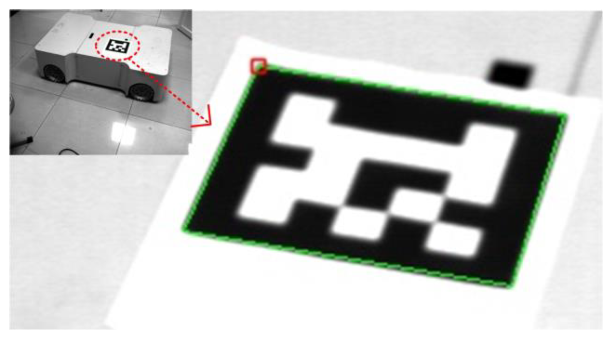
2.2.2. Corner Recognition and PnP Algorithm

The target for identification is a custom ceramic plate printed with ArUco code, the size of the ArUco code is 183 $\times$ 183 mm. It consists of a black border around and an internal binary matrix, the side length of each pixel block is 26.14 mm. The black border is conducive to rapid detection in the image, the internal binary matrix is beneficial to identify quickly and error correction. The upper left corner point in the figure is the mark point of the entire ArUco code. Mark point is the starting point of the corner point detection, and also the coordinate point for localization. The corner point detection is performed clockwise from the mark point. The coordinate value of the corner point represents the real-time coordinates of the AGV.

In the process of detecting the ArUco code, the image was first binarized based on an adaptive threshold. Then, a square contour was found and extracted from the binary image, which was transformed by perspective to restore its normal shape. The transformed image was separated into the white and black bits by using Ossu binarization. The specific dictionary type of the ArUco code is determined according to the black and white bits. After matching the correct ArUco code, with the marker point as the starting point, the four corner points are extracted clockwise. Combining the coordinate values of the four corner points in the image coordinate system and the world coordinate system, the PnP function in the OpenCV library is applied to solve the above rotation matrix R and translation matrix T to obtain the coordinate values of the landmark points in the world coordinate system. The solution method is the P3P algorithm. As shown in Figure 3, according to the cosine theorem:

$$\{\begin{array}{l}{L}_{O_c{P}_1}{}^2+L_{O_c{P}_2}{}^2-2\cdot L_{O_{c}P}{}_1\cdot L_{O_c{P}_2}\cos {\theta }_{P_1{O}_c{P}_2}=L_{P_1{P}_2}{}^2\\ L_{O_c{P}_1}{}^2+L_{O_c{P}_3}{}^2-2\cdot L_{O_c{P}_1}\cdot L_{O_c{P}_3}\cos {\theta }_{P_1{O}_c{P}_3}=L_{P_1{P}_3}{}^2\\ L_{O_c{P}_2}{}^2+L_{O_c{P}_3}{}^2-2\cdot L_{O_c{P}_2}\cdot L_{O_c{P}_3}\cos {\theta }_{P_2{O}_c{P}_3}=L_{P_2{P}_3}{}^2\end{array}$$

(9)

Divide all three expressions in Equation (9) by $L_{O_c{P}_3}{}^2$, make $x=\frac{L_{O{P}_1}}{L_{O{P}_3}},y=\frac{L_{O{P}_2}}{L_{O{P}_3}}$:

$$\{\begin{array}{l}{x}^2+y^2-2xy\cos {\theta }_{P_1{O}_c{P}_2}=\frac{L_{P_1{P}_2}{}^2}{L_{O{P}_3}}\\ y^2+1^2-2y\cos {\theta }_{P_1{O}_c{P}_3}=\frac{L_{P_1{P}_3}{}^2}{L_{O{P}_3}}\\ x^2+1^2-2x\cos {\theta }_{P_2{O}_c{P}_3}=\frac{L_{P_2{P}_3}{}^2}{L_{O{P}_3}}\end{array}$$

(10)

Make $v=\frac{L_{P_1{P}_2}{}^2}{L_{O{P}_3}},uv=\frac{L_{P_1{P}_3}{}^2}{L_{O{P}_3}},wv=\frac{L_{P_2{P}_3}{}^2}{L_{O{P}_3}}$:

$$\{\begin{array}{l}{x}^2+y^2-2xy\cos {\theta }_{P_1{O}_c{P}_2}-v=0\\ y^2+1^2-2y\cos {\theta }_{P_1{O}_c{P}_3}-uv=0\\ x^2+1^2-2x\cos {\theta }_{P_2{O}_c{P}_3}-wv=0\end{array}$$

(11)

Substituting the first expression in Equation (11) into the last two expressions:

$$\{\begin{array}{l}(1-u)y^2-u{x}^2-\cos {\theta }_{P_1{O}_c{P}_3}\cdot y+2uxy\cos {\theta }_{P_1{O}_c{P}_2}+1=0\\ (1-w)x^2-w{y}^2-\cos {\theta }_{P_2{O}_c{P}_3}\cdot x+2wxy\cos {\theta }_{P_1{O}_c{P}_2}+1=0\end{array}$$

(12)

where the three cosine values are known, u, w can be calculated by the coordinates of $P_1{P}_2{P}_3$ in the world coordinate system, x and y are unknown quantities. The above-mentioned system of binary quadratic equations about x and y are solved. Among the four sets of solutions obtained, the most suitable solution is selected, which is the obtained pose information. The recognition effect is shown in Figure 5.

2.3. Localization Method Fusion Complementary

Obstacles will easily block the FOV of the camera, causing the camera to fail to recognize the ArUco code on the AGV body. In this case, the host computer reads the UWB localization data sent by the Raspberry Pi as the current coordinates of the AGV. When the camera can accurately recognize the ArUco code, reading the localization data of the monocular camera as the coordinates of the AGV, it fulfills the localization requirements of the AGV in complex environments.

The data exchange is required at the moment when camera localization recognition is blocked. Since different localization method with a varied localization accuracy leads to a discontinuous localization trajectory, a mean compensation method is proposed to correct UWB localization data. The response time of both localization methods is at the millisecond level. The AGV moves at a speed of 0.2 m/s. At this speed, three consecutive sets of camera localization measurements can be viewed as three sets of data measured at the same position. At the moment of data switching, the host computer read the first three sets of camera localization data and record them as $(x_{c1},y_{c1})$,$(x_{c2},y_{c2})$,$(x_{c3},y_{c3})$, as well find the mean coordinates $(x_c,y_c)$. Similarly, the host computer read the first three sets of UWB measured data, record as $(x_{u1},y_{u1})$,$(x_{u2},y_{u2})$,$(x_{u3},y_{u3})$, and find the mean coordinates $(x_u,y_u)$. Then it subtracts coordinate $(x_u,y_u)$ from coordinate $(x_c,y_c)$ to get the error value $({\delta }_x,{\delta }_y)$ of the UWB localization relative to the camera localization. The calculation formulas are:

$$(x_c,y_c)=(\frac{1}{3}{\displaystyle \sum _{i=1}^3{x}_{ci},}\frac{1}{3}{\displaystyle \sum _{i=1}^3{y}_{ci}})$$

(13)

$$(x_c,y_c)=(\frac{1}{3}{\displaystyle \sum _{i=1}^3{x}_{ci},}\frac{1}{3}{\displaystyle \sum _{i=1}^3{y}_{ci}})$$

(14)

$$\{\begin{array}{l}{\delta }_x=x_c-x_u\\ {\delta }_y=y_c-y_u\end{array}$$

(15)

${\delta }_x,{\delta }_y$ are used as compensation factors to compensate for UWB localization data.

Subsequent UWB measured data are recorded as $(x_m,y_m)$, and the data corrected by the compensation factor are recorded as $(x_r,y_r)$. The compensation formula is:

$$(x_r,y_r)=(x_m+{\delta }_x,y_m+{\delta }_y)$$

(16)

The flowchart of the localization method is shown in Figure 6.

3. Localization Experiment Results and Analysis

3.1. Experimental Scheme Design

This test was performed in a room of 8 $\times$ 7 m. A UWB anchor and an industrial camera were installed on the four walls of the room respectively. The model of these industrial cameras is JHSM130Bs with 1.3 million pixels, 30 fps/s frame rate, and a resolution of 1280 $\times$ 1024 pixel. The center of the AGV was fixed with a UWB, and an ArUco code was printed on a custom ceramic plate. The AGV moved along a preset path in the center of the room. The schematic diagram of the measuring device is shown in Figure 7a. The physical diagram of the measuring device is shown in Figure 7b. The localization results of UWB and monocular cameras were recorded when the AGV was stationary at 30 specific coordinates respectively. As well, the curves of localization trajectory obtained by UWB and monocular camera were recorded when the AGV ran along the preset path. Then, the localization results were analyzed.

3.2. Static Localization Experiment

Within the scope of the room, a coordinate measurement point was selected every 120 cm. A total of 30 coordinate positions were set as static localization test points. Each position was repeatedly measured 100 times. The Euclidean distance between each sampling point and the coordinates set was calculated, which indicates the error generated by this localization. The calculation formula is:

$${\delta }_i=\sqrt{{(x_i-x)}^2+{(y_i-y)}^2}$$

(17)

where ${\delta }_i$ represents an error value, $x_i$,$y_i$ represents a measurement coordinate value, and x, y represents a set coordinate value. Among them, the error values of the coordinate (240, 240 cm) measured for one hundred times are shown in Figure 8. The average UWB localization errors of each coordinate point are shown in

Table 1. Ultra-wideband (UWB) localization average error of each coordinate point.

		X-axis
		120	240	360	480	600	720
Y-axis	120	(117.6,112.1) $\overline{\delta }$ = 8.25651	(242.0,127.4) $\overline{\delta }$ = 7.66551	(362.1,127.1) $\overline{\delta }$ = 7.40405	(477.3,113.1) $\overline{\delta }$ = 7.40945	(597.9,127.4) $\overline{\delta }$ = 7.69220	(717.3,128.5) $\overline{\delta }$ = 8.91852
	240	(122.2,247.6) $\overline{\delta }$ = 7.91201	(241.8,246.8) $\overline{\delta }$ = 7.03420	(361.8,246.6) $\overline{\delta }$ = 6.84105	(481.6,233.8) $\overline{\delta }$ = 6.40312	(601.9,247.0) $\overline{\delta }$ = 7.25328	(717.6,231.8) $\overline{\delta }$ = 8.54400
	360	(121.8,367.3) $\overline{\delta }$ = 7.51864	(241.7,366.6) $\overline{\delta }$ = 6.81542	(361.6,365.8) $\overline{\delta }$ = 6.07289	(481.6,354.4) $\overline{\delta }$ = 5.82409	(601.8,366.8) $\overline{\delta }$ = 7.03420	(717.8,367.5) $\overline{\delta }$ = 7.81601
	480	(122.1,472.1) $\overline{\delta }$ = 8.17435	(241.7,472.9) $\overline{\delta }$ = 7.30068	(361.7,486.0) $\overline{\delta }$ = 6.23618	(478.0,473.9) $\overline{\delta }$ = 6.41950	(601.9,486.9) $\overline{\delta }$ = 7.15681	(721.9,487.8) $\overline{\delta }$ = 8.02808
	600	(122.6,608.1) $\overline{\delta }$ = 8.50706	(242.2,607.2) $\overline{\delta }$ = 7.52861	(362.0,606.4) $\overline{\delta }$ = 6.70522	(482.0,593.6) $\overline{\delta }$ = 6.70522	(602.2,607.4) $\overline{\delta }$ = 7.72010	(717.4,608.3) $\overline{\delta }$ = 8.69770

, of which the unit is cm. The average camera localization errors at each coordinate point are shown in

Table 2. Camera localization average error at each coordinate point.

		X-axis
		120	240	360	480	600	720
Y-axis	120	(119.57,120.14) $\overline{\delta }$ = 0.45222	(239.35,120.13) $\overline{\delta }$ = 0.66287	(359.29,120.23) $\overline{\delta }$ = 0.66287	(479.28,120.26) $\overline{\delta }$ = 0.76551	(599.36,120.14) $\overline{\delta }$ = 0.75961	(720.44,120.13) $\overline{\delta }$ = 0.45880
	240	(119.37,240.17) $\overline{\delta }$ = 0.65253	(239.34,239.86) $\overline{\delta }$ = 0.67469	(359.18,240.27) $\overline{\delta }$ = 0.86331	(479.16,240.29) $\overline{\delta }$ = 0.88865	(599.32,240.18) $\overline{\delta }$ = 0.70342	(720.61,240.18) $\overline{\delta }$ = 0.63600
	360	(119.25,360.24) $\overline{\delta }$ = 0.78746	(239.13,360.27) $\overline{\delta }$ = 0.91093	(361.39,360.36) $\overline{\delta }$ = 1.43586	(478.73,360.34) $\overline{\delta }$ = 1.31472	(599.09,360.25) $\overline{\delta }$ = 0.94372	(720.78,360.23) $\overline{\delta }$ = 0.81320
	480	(119.38,480.18) $\overline{\delta }$ = 0.64560	(239.29,480.14) $\overline{\delta }$ = 0.72367	(360.84,480.24) $\overline{\delta }$ = 0.87361	(480.83,480.27) $\overline{\delta }$ = 0.87281	(599.23,480.18) $\overline{\delta }$ = 0.79076	(719.38,480.17) $\overline{\delta }$ = 0.64288
	600	(119.58,600.14) $\overline{\delta }$ = 0.44272	(239.36,600.14) $\overline{\delta }$ = 0.65513	(360.71,600.24) $\overline{\delta }$ = 0.74947	(480.71,600.27) $\overline{\delta }$ = 0.75961	(599.38,600.14) $\overline{\delta }$ = 0.63561	(720.43,600.16) $\overline{\delta }$ = 0.45880

, of which the unit is cm.

The localization results and setting values obtained by the two localization methods are shown in Figure 9. Figure 10 shows that for the difference of Y-axis coordinates, the average error $\overline{D}$ at the same X-axis coordinate is defined by Equation (18) when the X-axis coordinates are 120, 240, 360, 480, and 600.

$$\overline{D}=\frac{{\displaystyle \sum _{i=120,240,360,480,600}erro{r}_{Y=i}}}{5}$$

(18)

3.3. Dynamic Localization Experiment

The AGV traveled along a preset path. Obstacles in the path did not block the FOV of the camera. The measurement was repeated 10 times. The localization results of UWB and monocular cameras were recorded respectively. Figure 11 shows one of the localization results. Figure 11a shows relative to the results of the localization of the entire path. Figure 11b shows localization results relative to a path zoom. The red curve indicates the actual track in the figure. The green curve indicates the UWB localization trajectory. The blue dotted line indicates the camera localization trajectory. The distance, between the coordinates of the sampling point and the actual trajectory curve, represents the localization error. The average errors of the 10 localization results are calculated respectively, as

Table 3. Average errors of 10 localization results without occlusion.

Number	Monocular Camera Localization Error/mm	UWB Localization Error/mm
1	12.233	96.384
2	14.264	94.207
3	13.747	97.395
4	12.573	94.343
5	12.837	91.374
6	10.468	95.442
7	12.759	89.485
8	14.377	94.873
9	12.439	94.244
10	12.876	96.382

shows.

The camera was blocked for a time in the middle of the whole preset road to simulate the situation when the camera is blocked during the AGV driving. The measurement was repeated 10 times. The average errors of the localization results of the blocked road were calculated, as

Table 4. The average errors of 10 fusion localization results on the blocked road.

Number	Localization Error of Blocked Road/mm
1	47.436
2	51.357
3	53.583
4	49.437
5	50.422
6	44.382
7	62.593
8	45.873
9	47.795
10	48.376

shows. Figure 12 is a trajectory diagram of one of the localization results, in which the red trajectory is the localization trajectory of the occluded road section after the mean compensation method. Figure 13 is a comparison chart between the corrected data and the original data. It can be seen that the localization data of UWB is well corrected after the mean compensation method, which is closer to the standard value. Figure 14 shows the resulting trajectory of three localization methods. Figure 14a shows relative to the results of the localization of the entire path. Figure 14b shows localization results relative to a path zoom. The green curve in the figure indicates the UWB localization trajectory without the camera blocked. The blue dotted line indicates the camera localization trajectory without the camera blocked. The red curve indicates the actual trajectory of the AGV. The black dotted line indicates the merge localization trajectory of the two localization methods in the case of occlusion during the AGV driving.

Experimental data show that as the main localization method, in a situation that without obstructions, the localization of monocular camera can reach the static localization accuracy of 15 mm and the dynamic localization accuracy within 15 mm. The localization trajectory can perfectly coincide with the actual driving trajectory of the AGV. The mean compensation method is applied to compensate and correct the localization data of UWB when the FOV of the camera is blocked. It can be seen that the static localization accuracy with the only UWB is within 90 mm and the dynamic localization accuracy is within 100 mm. After correction, the dynamic localization accuracy can be reduced by half in theory. The experimental data verified this view that the average localization error of the covered road section is about 50 mm. The localization trajectory can maintain coherence at the instant of data exchange. The fusion of the two localization methods has a better effect, which meets the requirements of AGV positioning.

3.4. Effect of Camera Resolution on Experimental Results

To study the impact of the resolution of the camera on the localization accuracy, two additional cameras with a resolution of 640 $\times$ 480 pixels and 320 $\times$ 240 pixels were added for comparison experiments. Each camera was measured 100 times at the coordinates (240, 240 cm), the average static localization error was calculated to compare the static localization errors of different resolution cameras. Each camera was measured 10 times on the same path, obstacles in the path did not block the FOV of the camera. The average error was calculated to compare the dynamic localization errors of cameras with different resolutions. Each camera measures 10 times on the same path, the camera was blocked for a time in the middle of the whole preset road. And the average error was calculated to compare the fusion localization errors of cameras with different resolutions in the case of occlusion. The experimental results are shown in

Table 5. Camera localization test results at different resolutions.

Camera Resolution/Pixel	Average Static Localization Error at Coordinates (240, 240 cm)/cm	Dynamic Localization Error on Normal Road Section/mm	Dynamic Localization Error of Blocked Road Section/mm
1280 $\times$ 1024	0.675	12.857	50.125
640 $\times$ 480	1.572	19.374	66.581
320 $\times$ 240	3.351	45.718	89.743

.

Experimental data show that when the resolution is 1280 $\times$ 1024 pixel, high static localization accuracy, and dynamic localization accuracy can be achieved. When the resolution is decreased to 1/2, the localization accuracy is reduced. When the resolution is decreased to 1/4, both the static localization error and the dynamic localization error are relatively large. It can be seen that the use of a high-resolution camera can achieve a better localization effect, and the use of a low-resolution camera can reduce costs, but this results in a relatively large localization error. Therefore, when choosing a camera, the impact of resolution on the system should be fully considered.

Besides, the localization range of the UWB is about 100 $\times$ 100 m, and the FOV of the camera is the main factor affecting the scalability of the solution. Since each camera in this system is identified independently, when the room is large, the number of cameras can be increased to expand the localization area, which increases the scalability of the system.

4. Conclusions

This system of AGV indoor localization views the monocular camera as the main localization method while the UWB as an auxiliary localization method. The AGV was located by identifying the ArUco code fixed on AGV. This method avoids posting QR codes everywhere in the surrounding environment, as long as one ArUco code can realize the localization of the AGV. In the case that the FOV of the camera is blocked, UWB, as an auxiliary localization, is applied to ensure the coordinates of the AGV can be located at any time.

Compared with the most recent localization methods, LiDAR SLAM, this system has lower technical difficulty, lower cost, and higher localization accuracy on a path without obstructions. A comparison table of the two methods is shown in

Table 6. Comparison between the method of this article and the LiDAR SLAM localization method.

Method	Path Flexibility	Technical Difficulty	Precision	Cost
Method of this article	Good	General	High	General
LiDAR SLAM	Good	High	High	High

.

In general, the indoor localization system described in this article realizes the function of autonomous localization and navigation of the AGV in a storage environment.

In the future, we will continue to optimize this system, such as finding the best combination between the number of cameras and resolution to optimize performance and find the most cost-effective solution.

References

1. Long, J.; Zhang, C.L. The Summary of AGV Guidance Technology. Adv. Mater. Res. 2012, 591–593, 1625–1628. [Google Scholar] [CrossRef]
2. Moosavian, A.; Xi, F. Modular design of parallel robots with static redundancy. Mech. Mach. Theory 2016, 96, 26–37. [Google Scholar] [CrossRef]
3. Lu, S.; Xu, C.; Zhong, R.Y.; Wang, L. A RFID-enabled positioning system in automated guided vehicle for smart factories. J. Manuf. Syst. 2017, 44, 179–190. [Google Scholar] [CrossRef]
4. Yudanto, R.G.; Petré, F. Sensor fusion for indoor navigation and tracking of automated guided vehicles. In Proceedings of the 2015 International Conference on Indoor Positioning and Indoor Navigation (IPIN), Banff, AB, Canada, 13–16 October 2015. [Google Scholar]
5. Wang, L.; Guo, H. Exploring Key Technologies of Multi-Sensor Data Fusion; Atlantis Press: Paris, France, 2017. [Google Scholar]
6. Song, Z.; Wu, X.; Xu, T.; Sun, J.; Gao, Q.; He, Y. A new method of AGV navigation based on Kalman Filter and a magnetic nail localization. In Proceedings of the 2016 IEEE International Conference on Robotics and Biomimetics (ROBIO), Qingdao, China, 3–7 Decmber 2016. [Google Scholar]
7. Škrabánek, P.; Vodička, P. Magnetic strips as landmarks for mobile robot navigation. In Proceedings of the 2016 International Conference on Applied Electronics (AE), Pilsen, Czech Republic, 6–7 September 2016. [Google Scholar]
8. Sun, G.; Feng, D.; Zhang, Y.; Weng, D. Detection and control of a wheeled mobile robot based on magnetic navigation. In Proceedings of the 2013 9th Asian Control Conference (ASCC), Istanbul, Turkey, 23–26 June 2013. [Google Scholar]
9. Wang, C.; Wang, L.; Qin, J.; Wu, Z.; Duan, L.; Cao, M.; Li, Z.; Li, W.; Lu, Z.; Ling, Y.; et al. Development of a vision navigation system with Fuzzy Control Algorithm for Automated Guided Vehicle. In Proceedings of the 2015 IEEE International Conference on Information and Automation, Beijing, China, 2–5 August 2015. [Google Scholar]
10. Li, Q.; Hu, Z.; Ge, L. AGV Design Using Electromagnetic Navigation. Mod. Electron. Technol. 2012, 35, 79–81. [Google Scholar]
11. Xin, J.; Jiao, X.-L.; Yang, Y.; Liu, D. Visual navigation for mobile robot with Kinect camera in dynamic environment. In Proceedings of the 2016 35th Chinese Control Conference (CCC), Chengdu, China, 27–29 July 2016. [Google Scholar]
12. Ronzoni, D.; Olmi, R.; Secchi, C.; Fantuzzi, C. AGV global localization using indistinguishable artificial landmarks. In Proceedings of the 2011 IEEE International Conference on Robotics and Automation, Shanghai, China, 9–13 May 2011. [Google Scholar]
13. Wu, X.; Lou, P.; Tang, D.; Yu, J. An intelligent-optimal predictive controller for path tracking of Vision-based Automated Guided Vehicle. In Proceedings of the 2008 International Conference on Information and Automation, Shanghai, China, 20–23 June 2008. [Google Scholar]
14. Zhou, C.; Shuai, P.; Dai, C. The Application of QR Codes and WIFI Technology in the Autonomous Navigation System for AGV; Atlantis Press: Paris, France, 2018. [Google Scholar]
15. Zhou, C.; Liu, X. The Study of Applying the AGV Navigation System Based on Two Dimensional Bar Code. In Proceedings of the 2016 International Conference on Industrial Informatics—Computing Technology, Intelligent Technology, Industrial Information Integration (ICIICII), Wuhan, China, 3–4 December 2016. [Google Scholar]
16. Zeng, P.; Wu, F.; Zhi, T.; Xiao, L.; Zhu, S. Research on Automatic Tool Delivery for CNC Workshop of Aircraft Equipment Manufacturing. J. Phys. Conf. Ser. 2019, 1215, 012007. [Google Scholar] [CrossRef]
17. Weng, J.-F.; Su, K.-L. Development of a SLAM based automated guided vehicle. J. Intell. Fuzzy Syst. 2019, 36, 1245–1257. [Google Scholar] [CrossRef]
18. Wu, Z.; Wang, X.; Wang, J.; Wen, H. Research on improved graph-based SLAM used in intelligent garage. In Proceedings of the 2017 IEEE International Conference on Information and Automation (ICIA), Macau SAR, China, 18–20 July 2017. [Google Scholar]
19. Schueftan, D.S.; Colorado, M.J.; Bernal, I.F.M. Indoor mapping using SLAM for applications in Flexible Manufacturing Systems. In Proceedings of the 2015 IEEE 2nd Colombian Conference on Automatic Control (CCAC), Manizales, Colombia, 14–16 October 2015. [Google Scholar]
20. Zhang, J.; Lou, P.; Qian, X.; Wu, X. Research on Vision-Guided AGV Precise Positioning Technology for Multi-window Real-time Ranging. J. Instrum. 2016, 37, 1356–1363. [Google Scholar]
21. He, Z.; Lou, P.; Qian, X.; Wu, X.; Zhu, L. Research on Multi-Vision and Laser Integrated Navigation AGV Precise Positioning Technology. J. Instrum. 2017, 38, 2830–2838. [Google Scholar]
22. Zhang, H.; Cheng, X.; Liu, C.; Sun, J. AGV vision positioning technology based on global sparse map. J. Beijing Univ. Aeronaut. Astronaut. 2019, 45, 218–226. [Google Scholar]
23. Li, X.; Zhang, W. An Adaptive Fault-Tolerant Multisensor Navigation Strategy for Automated Vehicles. IEEE Trans. Veh. Technol. 2010, 59, 2815–2829. [Google Scholar]
24. Wang, H.; Zhang, X.; Li, X.; Han, L.; Zhang, J. GPS/DR information fusion for AGV navigation. In Proceedings of the World Automation Congress, Beijing, China, 6–8 July 2012. [Google Scholar]
25. Wei, Z.; Lang, Y.; Yang, F.; Zhao, S. A TOF Localization Algorithm Based on Improved Double-sided Two Way Ranging. DEStech Trans. Comput. Sci. Eng. 2018, 25, 307–315. [Google Scholar] [CrossRef]
26. Chen, P.; Wang, C. IEPnP: An Iterative Estimation Algorithm for Camera Pose Based on EPnP. Acta Opt. Sin. 2018, 38, 138–144. [Google Scholar] [CrossRef]
Figure 1. Time of flight (TOF) two-way ranging algorithm principle.
Electronics 09 00448 g001
Figure 2. Trilateral centroid localization algorithm.
Electronics 09 00448 g002
Figure 3. Schematic diagram of the world coordinate system and camera coordinate system conversion.
Electronics 09 00448 g003
Figure 4. Monocular camera localization diagram.
Electronics 09 00448 g004
Figure 5. Monocular camera localization recognition effect.
Electronics 09 00448 g005
Figure 6. Flow chart of the localization method.
Electronics 09 00448 g006
Figure 7. Flow chart of the localization method: (a) the schematic diagram of the measuring device; (b) the physical diagram of the measuring device.
Electronics 09 00448 g007
Figure 8. Coordinate (240,240) one hundred times localization error.
Electronics 09 00448 g008
Figure 9. Localization results and setting values obtained by two localization methods.
Electronics 09 00448 g009
Figure 10. Average errors of two localization methods.
Electronics 09 00448 g010
Figure 11. The localization result of UWB and monocular camera: (a) relative to the results of the localization of the entire path; (b) localization results relative to a path zoom.
Electronics 09 00448 g011
Figure 12. Location result tracking of the camera obscured road section.
Electronics 09 00448 g012
Figure 13. Comparison of corrected data and original data.
Electronics 09 00448 g013
Figure 14. Results of three localization methods: (a) relative to the results of the localization of the entire path; (b) localization results relative to a path zoom.
Electronics 09 00448 g014