1. Introduction
The 3D shapes recognition problem has been studied over a long period in the computer age with many applications in real life, such as robotics, autonomous driving, augmented/mixed reality, and so on. Many remarkable achievements in 2D object recognition have been made subsequently by the strong learning capability of a convolution neural network (CNN) and large-scale training datasets. Unlike conventional 2D images, there is a limit in the progress of 3D shape recognition [
1]. The reason is that a 2D manifolds’ representation of 3D models is not similar to the representation of 2D images.
The 3D models’ representation as 2D manifolds are not similar to 2D images representation, and a standard method to store the information of 3D geometrical shapes has not been developed [
2]. It seems hard to select deep learning techniques directly for 3D shape recognition. Unlike the general data formation of 2D images, the extraordinary formation of 3D shapes, such as Point Clouds and meshes as direct inputs for CNN, is one of the most challenging in CNN generalization from 3D shapes to 2D images [
3]. Presentations obtained for 3D shapes have significantly affected the performance of shape recognition.
Point Clouds and mesh are two main types of 3D shapes representation. Point Clouds representation has more benefits than 3D meshes in some ways. Firstly, Point Clouds are simpler and more uniform structures for a network to learn quickly. Secondly, Point Clouds allows easy applying of the deformation due to the independence of all the points as well as no requirement in updating connected information [
4]. Hence, the right choice for the classification task is directly generating 3D Point Clouds for the original 3D shape.
3D shape recognition is a base step that widely uses other tasks in intelligent electronic systems, such as 3D object tracking in intelligent robots or 3D object detection in autonomously driving cars. This paper will present the hybrid deep learning method, a combination of CNN and a Polynomial Kernel-based support vector machine (SVM) classifier, with a high accuracy in 3D shape recognition. CNN is used as the algorithm for feature extraction. The related studies are presented in section two before describing the method in section three. Then, we will compare other methods based on the numerical results. Finally, the conclusion is given.
3. Methodology
As shown in
Figure 2, the original 3D shape is first used for generating the 3D Point Clouds; these Point Clouds are rotated for the data augmentation and create the 2D projection. We use the hybrid deep learning network convolution neural network–support vector machine (CNN–SVM) for feature extraction and classification at the final step. Our method will be fully explained in the next section.
3.1. The Creation of 3D Point Clouds Data
We interpolate all vertices of the original 3D shape to produce the 3D Point Clouds. The 3D shape, including the faces and vertices, have file the formats STL, OBJ, and OFF. These file formats use the triangular faces with three vertices for each face.
Figure 3 shows the OFF file with only 41,285 vertices (without 22,034 faces).
We will interpolate 510 points
between two adjacent vertices
and
(
i = 1,2, …,
M − 1) among
M vertices
of the 3D shape using Equation (1). This interpolation technique will create 512 equally spaced points in the interval
.
Figure 4 shows the interpolation results of the original 3D shape. We can see that Point Clouds explore the interior designs such as chairs, the steering wheels, and the opposite wheels beside the reservation of the 3D shape boundary.
3.2. D Point Clouds Data Augmentation
As we have known, an insufficient amount of training data or unbalanced datasets are challenges in deep learning. Data augmentation, such as rotating, cropping, zooming, and histogram-based methods in conventional image transformation, are one method for solving these problems in 2D images classification [
23]. It is reasonable for us to extend to 3D from these 2D methods by choosing a rotation approach for 3D Point Clouds.
Figure 5 shows the original Point Clouds and Point Clouds after rotating by 90, 180, and 270 degrees, respectively.
We will normalize the 3D point by dividing all current elements in Point Clouds,
(a nx3 matrix with the number of points at n), by the maximum coordinate values of the
before the rotation. As a result, three coordinate values of Point Clouds will be inside the unit cubic (−1 <
x < 1, −1 <
y < 1, −1 <
z < 1).
Rodrigues' rotation formula [
24] is adapted to rotate the 3D Point Clouds, as given by Equation (3).
where
is the rotation matrix;
is the original Point Clouds;
is a rotated Point Clouds; RotAngle is the angle of the rotation in the degree;
H is the skew-symmetric;
h = (
) = ( 1 0 0 ); the rotation axis is Ox.
We rotate to obtain three more 3D shapes and four 3D shapes in total for each 3D shape in the dataset. Furthermore, we obtain four projections in total with a 32 × 32 × 3 size for each projection from each 2D projection of each 3D shape. The concatenation of these four projections along the third dimension produces a 32 × 32 × 12 matrix A as the input data of CNN.
3.3. The Architecture of CNN–SVM
The CNN–SVM architecture in the proposed method consists of an input layer, followed by four convolutional layers with 8, 32, 128, and 512 filters, respectively (see
Figure 6). We set values 1 for the padding for all convolutional layers, and the stride equals 1. Then, the fourth convolution layer is followed respectively by batch normalization and the rectified linear unit (ReLU) layer, and fully connected layer. Finally, CNN–SVM uses the SVM for the classification of the feature extract. There are some reasons for using the batch normalization layer in our network. Batch normalization not only speeds the training of neural networks but also allows to reduce overfitting by regularity, use the higher learning rates with fewer parameter initialization. A network’s activations over a mini-batch are normalized by batch normalization. More specifically, these activations subtract their means, all divided by their standard deviations. Hence, batch normalization is used to increase convergence speeds and to prevent model divergence [
25].
The first convolution layer, which inputs matrix A to apply a padding 1, and 1 × 1 stride-convolution function, produces eight feature maps traveling to the second convolution layer. The second, third, and fourth convolution layers produce 32, 128, and 512 feature maps with the dimensions of 34 × 34, 35 × 35, and 36 × 36, respectively. The output of the fourth convolution layer with a feature vector at size 512 is taken by the batch normalization layer. The output of the batch normalization layer moves to the ReLU layer, then to the fully connected layer.
The softmax activation function is employed in most of the deep learning models to predict and minimize cross-entropy loss in classification tasks. Tang et al. [
26] uses linear SVM instead of softmax for classification accuracy improvement on datasets, such as MNIST, CIFAR-10, and the ICML 2013. Softmax will be replaced by polynomial SVM in this paper. For each testing 3D shape, the SVM classification layer takes 128 feature vectors from the fully connected layer output and decides the corresponding class among
L classes (
L = 10 or 40).
The original problem of the SVM algorithm is binary classification, as seen in
Figure 1 (linear separable case). Suppose that we have a training data set (
), (
), …, (
), where
is the
i-th training data and
is the corresponding label. The equation of the hyperplane is
. The nearest red point to the hyperplane satisfies
. If the new data point satisfies
it will belong to the red class (class 1), and vice versa.
SVM’s problem in binary classification is to find
w and
b so that the margin is maximized. The SVM problem is defined as a quadratic optimization problem, shown in formula six.
The dual form is defined as
The data is normally non-linear for multi-classification, and SVM transforms non-linear data to linear by using mapping function, namely,
. This mapping transforms original data to a higher dimension space that is linearly separable. The term
in Equation (7) is replaced by
in the multi-classification problem. Practically, it is unnecessary to calculate
for all data points, so we need to calculate the only
for any two data points. From this point, the concept kernel,
is introduced. The polynomial kernel in this study is defined in the following equation.
This study uses a one-versus-one approach for multi-classification SVM, which constructs pairwise binary classifications SVM (L is the number of classes). The most frequent predicted class, which wins most among these pairwise binary classifications for one-versus-one multiclass SVM, is defined as the final prediction for a test point. Let consider an example with L = 4, and the four classes, namely, A, B, C, and D. Multi-classification SVM will use six binary classifications SVM to predict the class of a test point. The first binary classification will determine whether a test point belongs to class A or B. Similarly, the remaining five binary classifications will predict whether a test point belongs to class A or class C, class A or class D, class B or class C, class B or class D, and class C or class D. Suppose that the results for six binary classification SVM are B, A, D, B, B, D, then the final prediction will be class B with the highest frequency (frequency is 3).
4. Experimental Results
Our experiments will work on the ModelNet dataset, including ModelNet10 and ModelNet40 [
16]. The original ModelNet dataset can be downloaded from the website in the
Supplementary Materials. The 3D CAD of ModelNet10 has ten categories with 3991 training and 908 testing models, comparing forty categories with 9843 training and 2468 testing models from the 3D CAD of ModelNet40. OFF is a 3D-triangle mesh format of each CAD model of ModelNet. The number of models of a specific class for the ModelNet40 is shown in
Table 2. In case that the model has less than 128,000 vertices, all CAD models in the original dataset are interpolated. If the model has more than 128,000 vertices, the original model is still kept without interpolation due to the differences in the number of model vertices in the same class. For example, the airplane class has the maximum vertices at 2,286,376 and the minimum at 1107 before interpolation, so the ratio is 2,286,376/1107 = 2065.38. After the interpolation process, we have 1106 × (510) + 1107 = 565,167 total points, and the ratio is 2,286,376/565,167 = 4.05.
Figure 7 shows the 2D projections from the 3D rotation on 3D Point Clouds of random models in the ModelNet40 dataset.
We implemented all experiments on the computer I7 7700, 32GB memory, 1080Ti GPU, windows 10, MATALB (9.7 (R2019b), Natick, MA, USA). The network is trained by choosing Adam optimization Algorithm at the momentum 0.9, at the mini-batch size 16, and with the initial learning rate 0.000001. The polynomial kernel is used in SVM with the hyperparameters at degree 2, gamma 0.001, and cost 1. The training time for ModelNet10 and ModelNet40 is 4.5 hours and 15.5 hours, respectively.
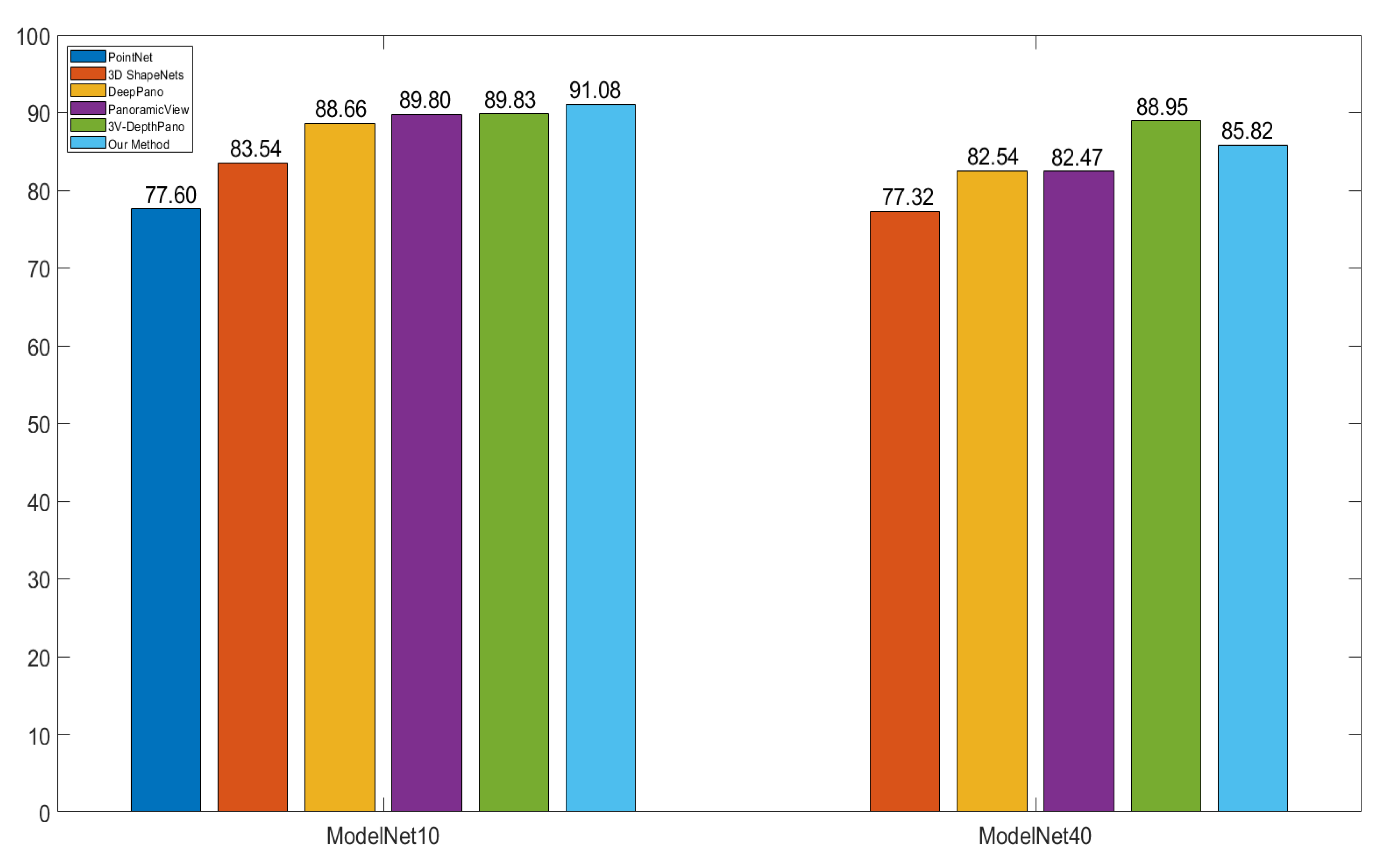
Figure 8 shows that our method is more accurate than others with precision at 91.08% and 85.82% for ModelNet10 and ModelNet40, respectively. The PointNet and 3D ShapeNets have the lowest precision levels, with 77.60% on the evaluation of only the ModelNet10 dataset for the PointNet, and with 83.54% on ModelNet10 and 77.32% on ModelNet40 for the 3D ShapeNets.
The PointNet and 3D ShapeNets work with the voxel, which has a 30 × 30 × 30 minimum size for each 3D shape. In Matlab, the default class double requires eight bytes per element of memory for storage. Hence a 3D matrix of size 30 by 30 by 30 takes 0.206 Mb of memory. In contrast, the proposed method describes each 3D shape by a 32 ×32 × 12 matrix, and thereby takes 0.094 Mb of memory (half the size of the voxel approach). DeepPano, PanoView, and 3V-DepthPano belong to the group of the view-based method. In these three methods, a cylindrical surface whose central axis concurs the principal axis of the model surrounds the 3D model for building a panoramic view. DeepPano and PanoView construct a panoramic view from one key view, while 3V-DepthPano uses three different panoramic views from three key views. 3V-DepthPano gains the highest accuracy but requires the largest input data size at 227 by 227, which consumes 0.393 Mb of memory, is four times the memory of the proposed method. Moreover, 3V-DepthPano is the only method which uses parallel CNN structure with three-branch CNN, causing the high complexity of deep learning network. The proposed method could get better accuracy without constructing a cylindrical surface and panoramic view because it directly captures a single 2D projection of 3D interpolation Point Clouds based on the linear interpolation algorithm. In addition, the proposed method uses single CNN instead of multi-branch CNN. Furthermore, our method contains more spatial information with a single 2D projection, such as the opposite side of the cone and Flower Pot, as seen in
Figure 7.
There is at least one parameter in the pooling layer and no parameters in batch normalization and the ReLU layer for all other methods. There are five convolution layers in the 3V-DepthPano which use the Alexnet model [
27]. Both Panoramic View [
3] and DeepPano use four convolution Blocks with one convolution layer for each block, followed by a max-pooling layer, compared with four convolution layers in our method. The number of parameters in the fully-connected layers is not compared because there is no information on the number of feature vectors of this layer in the DeepPano method in [
17]. The first and second layers of the Panoramic View used 512 and 1024 feature vectors, respectively, while both layers of the 3V DepthPano method had 4096 vectors. Unlike these methods, one fully connected layer with 128 feature vectors will be used. Our method used fewer parameters at 3400 in total for all convolution layers than their methods with 18,112 for DeepPano, 15,088 for Panoramic View, and 28,608 for 3V-DepthPano (see
Table 3). Therefore, our method is more efficient because it reduces model parameters, and as a result, diminishes the computational cost. Panoramic View and DeepPano choose parameters approximately equal and have similar accuracy at 82.54% and at 82.47%, respectively, for ModeleNet40. Panoramic View made a 1.14% accuracy increment in the classification task on ModelNet10, compared with DeepPano, and has the same accuracy with 3V-DepthPano. Because 3V-DepthPano has twice as many parameters as Panoramic View, it shows a 6.49% higher accuracy in the ModelNet40 classification.
Our method is more accurate on ModelNet40 than on other methods, except 3V-DepthPano. The main reason is that the number of parameters in 3V-DepthPano, namely, 28,608, is 8.41 times the corresponding parameters in our method, and the 3V-DepthPano used the highest input at a 227 x 227 size.
Figure 9 shows a confusion plot for ModelNet10 and ModelNet40. The most misclassified percentages are 25% for the Flower Pot class and 40% for the Cup class. Flower Pots are misclassified as Plants at 50%, and Cups are predicted as vases at 20%. The data representation helps our methods to obtain the highest accuracy in the ModelNet10 dataset, as shown in
Figure 8. DeepPano used only one view, while 3V-DepthPano had complete information in three views. This is one of the reasons why 3V-DepthPano outperforms DeepPano. The information of the 3D shape in our method is explored externally and internally; for example, the interior designs of the car class is stored. Therefore, the proposed method achieved higher accuracy.
The proposed method performs best, except that the recognition for the cup object class still has a low accuracy. The imbalance between classes in the dataset in the study may affect the results. The rate of success in object recognition is opposite with an increase and a decrease in a higher and a lower number of training samples, respectively. Oversampling techniques could handle the class imbalance and reduce uncertainties in the minority classes because it adds an amount to the training data for these classes. The direction for future research is that we design new oversampling techniques to eliminate the imbalance between classes.
The object recognition method in this study can work with an intelligent robot using the Microsoft Kinect sensor. At the initial step, the robot could not recognize various objects such as a person, cup, bottle, and desk in the scene. Next step, the robot queries the feature vectors of the offline dataset; these feature vectors are extracted by using the proposed method. Then, the robot assigns the labels for the extracted features from the constructed 3D object. This 3D object is captured by the Kinect sensor. Finally, the robot can fully recognize objects.


