Article

Trajectory Prediction and Channel Monitoring Aided Fast Beam Tracking Scheme at Unlicensed mmWave Bands

1
Beijing Laboratory of Advanced Information Network, Beijing Key Laboratory of Network System Architecture and Convergence, Beijing University of Posts and Telecommunications, Beijing 100876, China
2
DOCOMO Beijing Communications Laboratories Co. Ltd., Beijing 100190, China
*
Author to whom correspondence should be addressed.
Electronics 2020, 9(5), 747; https://doi.org/10.3390/electronics9050747
Submission received: 20 March 2020 / Revised: 21 April 2020 / Accepted: 28 April 2020 / Published: 1 May 2020
(This article belongs to the Special Issue Massive MIMO for 5G)

Abstract

:
Unlicensed 60 GHz millimeter band has a great potential in industrial Internet of things (IIoT) owing to its continuous large bandwidth. However, the signal transmission in this band suffers from high propagation loss, thus beamforming is adopted to provide directional gain. With the increasing number of beams, beam alignment and tracking in mobility scenario may incur unacceptable latency and overhead, and the existing beam management mechanism is no longer suitable. To reduce the latency and signaling overhead during beam tracking, we propose a fast beam tracking scheme with the help of trajectory prediction and channel monitoring. More specifically, we firstly quantify the beam coherent time to reduce the frequency of beam searching. Then, a two-stage heuristic trajectory prediction and channel monitoring aided fast beam tracking scheme is proposed to obtain the optimal beam pairs in the process of terminal movement and make sure that the interference on the directional beam is under the limit. Simulation results verify the effectiveness of the beam coherent time and the advantages of the proposed scheme in terms of complexity, outage probability, and effective spectrum efficiency.

1. Introduction

With the development of wireless communication system, the next industrial revolution is on the way. The fifth generation (5G) communication technology brings the industrial Internet of things (IIoT) into the era of Industry 4.0 [1]. Head mounted displays, handheld terminals, collaborative robots, and automated guided vehicles (AGV) are widely deployed in industrial factory to achieve more intelligent information interaction. Due to the exponential growth of mobile data traffic, the problem of spectrum scarcity is getting worse. To meet the requirements of IIoT, unlicensed 60 GHz spectrum has aroused extensive attention due to the continuously available spectrum resources [2]. However, the signal transmission in this band suffers from high propagation loss [3]. Therefore, large-scale antenna should be used to improve the diversity gains at the transceiver [4].
To further extend the coverage range, beamforming techniques are also adopted to provide directional gain. Typically, the hybrid beamforming architecture is used to realize massive multiple-input multiple-output (MIMO) due to the high cost of RF chains and power consumption in traditional full-digital beamforming [5]. Considering the difficulty to acquire perfect channel state information (CSI), the analog beamformer usually performs beam alignment through a specific pre-defined codebooks. Although the codebook-based beam alignment techniques are more convenient to be adopted on the inexpensive RF phase shifters, the latency and signaling overhead will be increased during beam management [6,7].
Compared with the static scenario, beam misalignment probability increases greatly in a dynamic IIoT environment. The communication links are prone to interruption due to the rapid changes of mobile user’s location. To update and reconstruct the communication beam, some beam tracking methods have been proposed in the literature. The three-stage search method in [8] narrows the beam range step by step to reduce the time complexity. However, when the size of antenna arrays increases, the time complexity of this method is still very high. Two pre-established codebook fingerprints are constructed in [9] to obtain the optimal beam pairs at the current location. Although the proposed method provides high performance with larger antenna arrays, the database construction is time consuming. Since communication is mainly through LOS component in dynamic scenario, its beam direction can be tracked based on the user’s location and velocity. Prior works developed in [10,11,12,13,14] attempt to obtain location of the user to track the beam. The angle of arrival (AOA) and angle of departure (AOD) can determine the channel, which can then be used to construct the optimal beamforming precoding vector directly [11]. To achieve accurate location information, an uplink time-difference-of-arrival (TDOA) measurement is considered in [12] at multiple Remote Radio Heads (RRHs). In addition, to track and predict the position more precisely, the Extend Kalman Filter (EKF) is adopted. Device Positioning is another way to get a user’s location, which can be achieved by global navigation satellite-based systems (GNSS), radar, cameras, and laser scanners (lidar) [13,14].
With the use of larger antenna array and narrower beams at unlicensed 60 GHz spectrum, a higher latency and signaling overhead of the beam tracking will be caused by the increasing of the number of beams. To deal with this problem, in addition to reducing the complexity of the beam tracking algorithm, a suitable beam switching time should also be found to minimize the signaling overhead. To the best of our knowledge, there are few studies aiming to investigate the update frequency of beam alignment during terminal motion. It is naturally to leverage channel coherence time for beam alignment. However, the channel coherence time is only a few milliseconds or less at the 60 GHz mmWave bands. As a result, it is impossible to align beams by the channel coherence time in terms of the frame structure in the 5G protocol. To determine a suitable beam switching time, we derive the beam coherent time. Moreover, we propose a trajectory prediction and channel monitoring aided fast beam tracking (TCFBT) scheme to further reduce the latency and overhead for beam alignment. In other words, we first derive a beam coherent time to reduce the frequency of beam alignment. Then, a Gaussian process-based sector prediction algorithm is presented to narrow the scope of beam searching. Finally, the optimal beam pairs are selected by the joint directional Listen before talk (LBT) and beam training algorithm proposed in the following.
In conclusion, the main contributions of this paper can be summarized as follows:
  • We derive the beam coherent time based on DFT codebook to indicate the terminals switching their beams. Moreover, we quantify the beam pointing error and the beam coherence time and discover that the beam coherence time is much longer than the mmWave channel coherence time. Consequently, the beam coherence time is more suitable for beam tracking with mobile terminal.
  • We propose a two-stage heuristic TCFBT scheme to ensure the fairness and availability of the beams for 5G mobile terminal in unlicensed 60 GHz. In other words, a Gaussian process-based sector predict algorithm is adopted to determine the corresponding sectors at the transceivers in the first stage. Then, a joint directional LBT and beam training algorithm is proposed in the second stage to obtain the optimal beam pair links in the current moment. The proposed scheme reduces the searching range of the beam set by trajectory prediction and channel monitoring. Therefore, the latency and overhead are further reduced to a large degree.
The symbolic notation we use in this paper is shown in Table 1.
The rest of this paper is organized as follows. In 
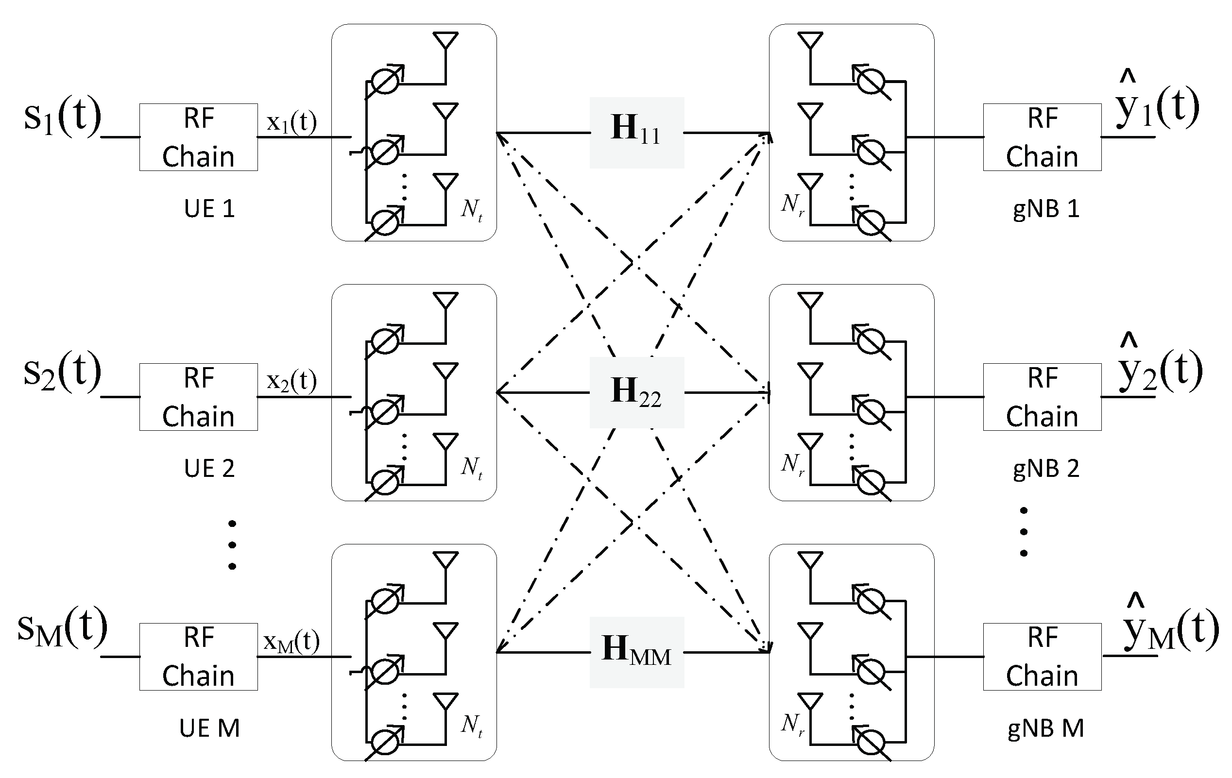
Section 2, the considered system model is described, including the multi-user single links in mobility scenario, receive signal structures with analog beamforming and channel model. To reduce the frequency of beam searching, the beam coherent time is derived in Section 3. In Section 4, we present the TCFBT scheme, including a Gaussian process-based prediction algorithm and the joint directional LBT and beam training algorithm. After that, the performance of our algorithm is evaluated by the system-level simulations in Section 5, while the conclusions are drawn in Section 6.

2. System Model

2.1. Multi-User Single Links in Mobility Scenario at 60 GHz

We consider a multi-user single links communication system in an industrial factory building with low mobility. The transceivers are equipped with massive MIMO systems. As shown in Figure 1, assume that there are M 5G mobile users (UEs) communicating with the corresponding gNBs at 60 GHz using directional beams. An uplink transmission scenario is considered to analyze the signal transmission characteristics, while the conclusion can be easily extended to the downlink transmission.
We assume there are N s transmitting antennas on the UE side and N r receiving antennas on the gNB side. Here, only one RF chain is considered to form directional links and we only focus the beam tracking in a single gNB. The analog precoding vector on the ith UE at time t is denoted by f i , t ( N s × 1 ) at the transmitter, and the combining vector on the ith gNB at the same time is regarded as w i , t ( N r × 1 ) at the receiver. The definition also applies to f j , t , w j , t .
According to the signal transmission model in Figure 2, the transmitted signal vector x i ( t ) is therefore given by
x i ( t ) = f i , t s i ( t ) ,
where s i ( t ) is the data transmitted from UE i to gNB i at time t, which should also obey E [ | s i ( t ) | 2 ] = 1 .
For the ith gNB, the final processed signals y ^ i ( t ) at the gNB can be written as
y ^ i ( t ) = w i , t H H i i ( t ) f i , t s i ( t ) + j = 1 , j i M w i , t H H j i ( t ) f j , t s j ( t ) + w i , t H n ( t ) ,
where s j ( t ) is the interference signal transmitted from other 5G users. It should be noticed that these interferences include mainlobe and sidelobe interference, which depend on the relative position of the gNB and UE at the current time. The dashed lines in Figure 2 represent the interference links, while the solid lines are the desired signals from UE to the corresponding gNB. n ( t ) is Gaussian white noise that follows i.i.d C N ( 0 , δ 2 ) .

2.2. Channel Model

Considering a common geometric mmWave channel model, the spatiotemporal multipath mmWave sparse channel is given by [15]:
H ( t ) = N s N r N c N l c l α c , l a r φ c , l r ( t ) a s H [ φ c , l s ( t ) ] e j 2 π v l t ,
where N c and N l represent the number of clusters and the rays of channel, respectively. α c , l denotes the complex gain on cth cluster, lth ray, with zero means and χ c 2 variance, where χ c is the power of each cluster and c χ c 2 = N c N l . a r φ c , l r ( t ) and a s φ c , l s ( t ) represent the normalized array response vectors at the receiver side and the transmitter side, respectively. φ ( t ) is the corresponding azimuth angle at time t. Then, we get the channel gain E [ | | H | | F 2 ] = N s N r . e j 2 π v l t represents the doppler shift and v l represents the speed on each path of the channel. We adopt a uniform linear array (ULA) at the transceiver, the array response vector can be expressed as
a φ ( t ) = 1 N [ 1 , , e j 2 π λ d ( p sin φ ( t ) ) , , e j 2 π λ d ( ( N 1 ) sin φ ( t ) ) ] ,
where p = 0 , . . , N 1 is the antenna element index on the antenna panel. λ is the wavelength and d = λ / 2 represents the distance between antennas. N is the number of antennas which can be recognized with N s or N r .

2.3. Problem Formulation

When the data transmit over the narrowband block-fading mmWave channel during a period of time, the ergodic capacity of the communication networks can be denoted as
C = E [ i = 1 M log 2 ( 1 + | w i , T H H i i ( T ) f i , T | 2 j = 1 , j i M | w i , t H H j i ( t ) f j , t | 2 + | w i , T H | 2 δ 2 ) ] ,
where E [ · ] represents the expectation of the network capacity over different fading channel states due to the movement of UE. Assume that the users switch the beams during each beam switching time T B , we define T = 1 , 2 , , as the index of the beam switching time.
To obtain the optimal analog precoding matrix and the combining matrix at each beam switching time, the transceivers have to exhaustively search all the possible beam pairs. The UE should switch their beam pairs to maintain the capacity of communication systems according to the physical location. Therefore, we define a latency factor to quantify the impact of signaling overhead for beam switch, which is denoted as η = ( T B T s ) \ T B , where T s is the beam searching time. Then, the effective ergodic capacity is written as η C . We formulate the following optimization problem
{ w i , T , f i , T , T B , T s } = arg max η C s . t . w R F i , T W f R F i , T F j = 1 , j i M | w i , t H H j i ( t ) f j , t | 2 β t h
where F and W are the corresponding beamforming codebooks on the transmitter and the receiver, respectively. β t h is denoted as the clear channel assessment (CCA) threshold of directional LBT to guarantee an idle channel. This problem is a non-convex optimization problem, and it is hard to obtain the global optimal solution. To this end, we derive a more appropriate beam coherent time to reduce the frequency of beam alignment in Section 3. Then, a two-stage heuristic TCFBT scheme is proposed in Section 4 to further decrease the beam searching time T s . The optimal beam pairs can be selected by joint directional LBT and beam training algorithm designed in TCFBT scheme.

3. Beam Coherent Time

In the process of terminal movement, it is much more frequent to switch beam according to channel coherent time. To determine a more reasonable beam switching time, we first quantify the beam pointing error and the beam coherence time for the LOS cases in this section. Then, two types of function are proposed to fit the probability density function (PDF) of antenna pattern. It should be noticed that the analysis is based on a single link, while the derived beam coherent time is also applicable to multiple links since the time is only related to the user’s speed, time, and beam direction (or the beam width).
The model we use to evaluate the beam misalignment is the two-dimensional motion model shown in Figure 3. Let the UE point at gNB have beam direction θ ( t ) at time t and move with a constant speed v along the straight line to reach point B at time t + τ . Take the UE side as an example; the beam pointing error is defined as Δ θ = θ ( t + τ ) θ ( t ) over a short period of time τ . As a result, the distance from A to B can be denoted as v τ . Assuming the distance from the gNB to the UE is S at time t, we quantify the relationship between the user’s speed, time and beam direction according to the law of sines for triangle, i.e.,
S s i n ( θ ( t + τ ) ) = v τ s i n ( Δ θ ) .
When the angle Δ θ is small, s i n ( Δ θ ) Δ θ , the beam pointing error is derived as
Δ θ = v τ S s i n ( θ ( t ) ) .
To evaluate the relationship between beam pointing error and receive power, we introduce the concept of beam coherence time. It is defined as the average time that the beam can stay aligned [16]. In other words, when the received power P at time t + τ drops to a certain degree compared with the power at time t due to channel variation, it is considered that the beam misalignment occurs at this time. In this case, T B = τ is defined as the beam coherence time, i.e.,
T B = i n f { τ | P t + τ P t < ξ t h } ,
where ξ t h is the threshold representing the decline degree of the received power. Because the power is proportional to the beam pattern G, Equation (9) can be written as ξ t h = G θ + Δ θ / G θ at beam switching moment. Moreover, we adopt a specific DFT codebook [17] as a predefined codebook to generate the communication beam pattern. The codebook can be generated by
F ( m , n ) = 1 N exp ( j 2 π N m n ) ,
where m = 0 , . . , N 1 and n = 1 , , N 1 represent the antenna element index and the beam pattern index, respectively.
Since the received power P can be expressed as the gain of antenna beam pattern approximately, the study in [
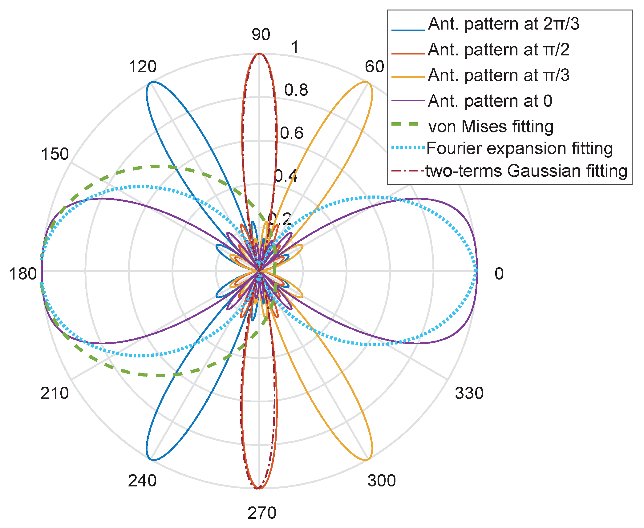
16] adopts von Mises distribution to fit the probability density function (PDF) of antenna beam pattern. However, von Mises cannot fit the antenna beam pattern exactly. As a result, we select Fourier expansion of triangular (FET) and two-term Gaussian function (TGF) to fit the PDF of DFT beam pattern more accurately. The fitting functions are shown as
G θ F E T = a 0 + a 1 cos ( w θ ) + b 1 sin ( w θ ) , G θ T G F = a 1 e ( θ b 1 c 1 ) 2 + a 2 e ( θ b 2 c 2 ) 2 ,
where a 0 , a 1 , a 2 , b 1 , b 2 , c 1 , c 2 , w are regression coefficients under the confidence probability of 95 % which can be calculated by least square estimator. As shown in Figure 4, the root mean square error (RMSE) in FET fitting is 0.1638 for the first column vector with the largest beamwidth in DFT codebook. The fitting precision becomes better as the number of Fourier expansion terms increases. For the other column vector in DFT codebook, the RMSE in TGF fitting is 0.103 . Both are much smaller than the von Mises distribution (RMSE with 0.3147 for the first column vector) proposed in [16]. It should be noticed that the FET fitting is appropriate for the case where the beamwidth is greater than or equal to π / 3 , and TGF fitting is suitable for the beams with beamwidth less than π / 3 . Taking FET fitting as an example, the beam coherence time is
T B = S v sin ( θ ) a 0 + a 1 cos ( w θ ) + b 1 sin ( w θ ) a 1 sin ( w θ ) b 1 cos ( w θ ) w 1 ξ t h ,
and the derivative process can be seen in Appendix A.
Therefore, the beam coherent time is then defined as the corresponding beam switching time. Instead of switching beams in each shorter channel coherent time, the UE only need to switch their beams at the beginning of each beam coherent time, which can reduce the latency and overhead to a large extent.

4. Trajectory Prediction and Channel Monitoring Aided Fast Beam Tracking Scheme

As discussed above, we derive an appropriate beam coherent time to decrease the frequency of beam alignment. In this section, we propose a two-stage heuristic TCFBT scheme to reduce the latency T s in the problem in Equation (
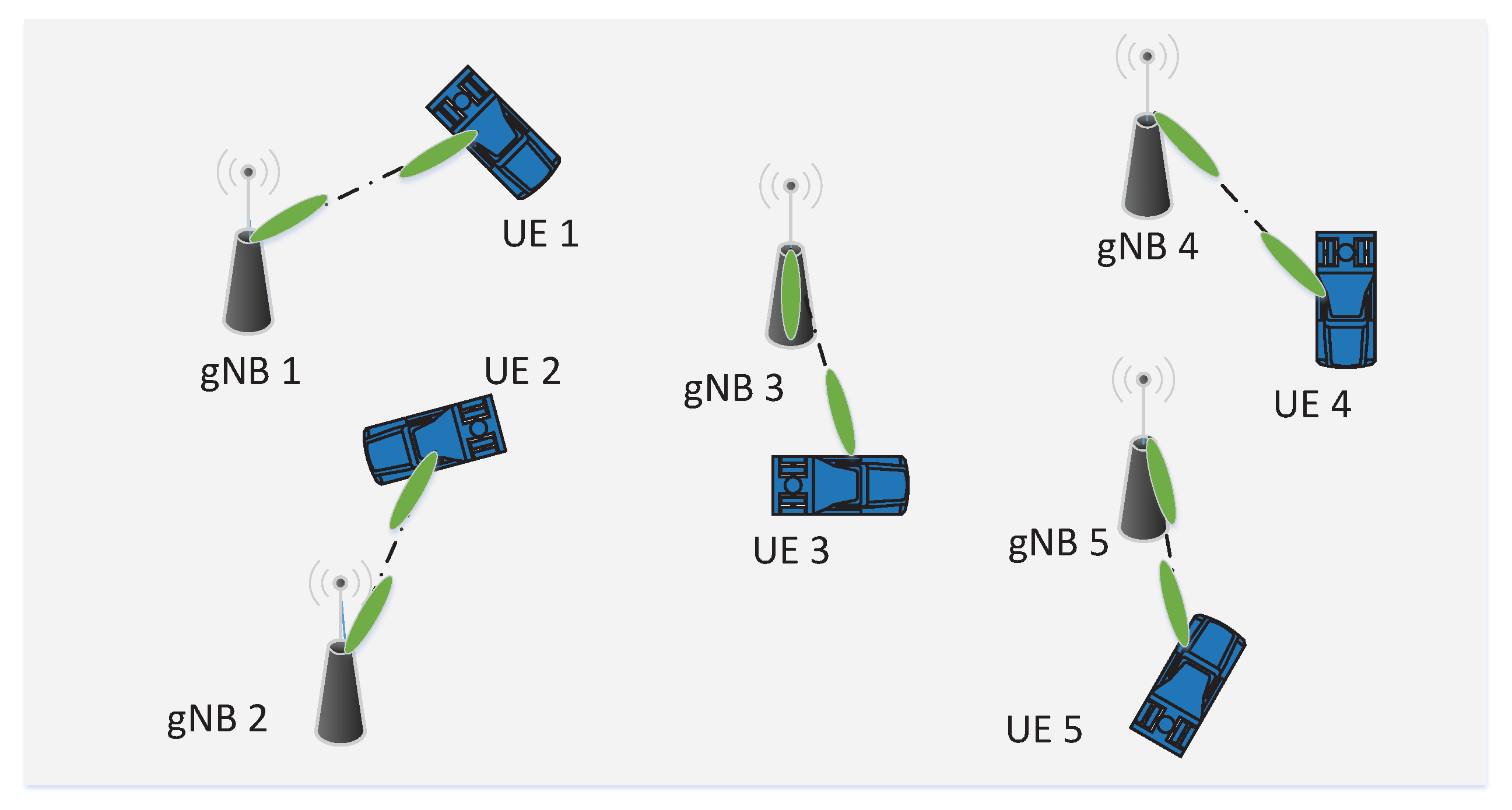
6) and signaling overhead in the process of beam training. A sector prediction algorithm based on Gaussian process classifier is adopted in the first stage to acquire the beam subset, which reduces the space of beam training and is more suitable for beam tracking in mobile scenario. Then, we leverage directional LBT in the second stage to further decrease the range of beam training. To be more specific, we divide the 360-degree spatial region of the transceiver into a limited set of sectors, and the sector prediction algorithm is used to predict the sector indices of the transceivers. After that, the joint directional LBT and beam training algorithm (JDLBT) is used in the selected sector to obtain the optimal beam pair. Finally, we analyze the complexity of the proposed two-stage scheme.

4.1. Gaussian Process-Based Sector Prediction Algorithm

In the light of the study in [18], a Gaussian process is a collection of random variables, any finite number of which have a joint Gaussian distribution. Therefore, we adopt the GP-based machine learning algorithm to build a prediction model for coordinate prediction. The aim of the GP-based algorithm is to find the input-output mappings of the position coordinates from the observation data. After that, we use the geometric model described in Section 4.1.1 and Section 4.1.2 to establish the relationship between position coordinates and sectors.
Considering a standard GP regression model,
z = f ( x ) + n ,
where x is the one-dimension coordinate value of each mobile user in the xy-plane and z is the output predicted coordinate value on the same direction. f ( ) is the regression function with the mean function of m ( x ) and covariance function k ( x , x ) . n is the Gaussian noise that follows i.i.d C N ( 0 , δ 2 ) .
Define a training set Γ with length L, Γ = ( X , Z ) , where X = [ x 1 , , x L ] is a matrix of input coordinate value and Z = [ z 1 , , z L ] is a matrix of output predicted coordinate value, respectively. For each x l ( l = 1 , , L ) , it represents the historical observations during each beam coherent time T B and can be denoted as x l = [ x ( t 1 ) , , x ( t Δ t ) ] T . z l = [ z ( t ) , , z ( t + Δ t ) ] T is defined as the predicted coordinate value during the same beam coherent time T B . It should be noticed that X can be represented by either x-coordinate value or y-coordinate value of the mobile user in the xy-plane here. Assuming that the input of test dataset is X and the output is Z , the distribution with the zero mean function can be written as
[ Z , Z ] T N ( 0 , [ K ( X , X ) + δ 2 I L , K ( X , X ) K ( X , X ) , K ( X , X ) ] ) ,
where K ( ) represents the covariance function. As a result, the prediction distribution can be denoted as
P ( Z | X , Γ ) N ( K ( X , X ) ( K ( X , X ) + δ 2 I L ) 1 Z , K ( X , X ) K ( X , X ) ( K ( X , X ) + δ 2 I L ) 1 K ( X , X ) ) .
The predicted coordinate value can be obtained by the mean function in Equation (15), which means the predicted coordinates can be achieved by using expression x ^ u ( y ^ u ) = K ( X , X ) ( K ( X , X ) + δ 2 I L ) 1 Z . Then, the following two steps can be processed to predict the corresponding sector.
As shown in Figure 3, we assume that the coordinate of UE is ( x u , y u ) , and the coordinate of gNB is ( x b , y b ) . The initial pointing direction ϑ at UE side is denoted as ϑ ( t ) . As a result, we derive t a n ϑ ( t ) = y u y b x u x b . Assume that the transceivers pre-divide the beam radiation space into eight sectors. Take the transmitter as an example, the relationship between coordinate and the antenna sector can be obtained by using the following steps.

4.1.1. Step 1

First, the transmitter should determine the range of the AOD. When x u x b < 0 , it indicates ϑ ( t ) [ π 2 , π 2 ] . If x u x b = 0 , y u y b < 0 , it represents ϑ ( t ) = π 2 , and, if x u x b = 0 , y u y b > 0 , ϑ ( t ) = π 2 . When x u x b > 0 , it means ϑ ( t ) [ π 2 , 3 π 2 ] .

4.1.2. Step 2

Then, the transmitter will calculate the AOD by ϑ ( t ) = a r c t a n y u y b x u x b . After that, the transmitter will search the range of sector sets to determine the sector index based on the corresponding ϑ ( t ) .
After sector prediction, each 5G mobile user i and the corresponding gNB i can select their optimal beam pairs from the beamforming codebooks in the predicted transceiver sectors, and this subset is denoted as F s and W s , respectively.

4.2. Joint Directional LBT and Beam Training Algorithm

Although the size of beam training set decreases, we can also use directional LBT to further narrow the scope of beam training. Therefore, we design a JDLBT algorithm to obtain the optimal beam pairs. Specifically, the transceivers execute directional LBT on the beam training subset W s , F s , which are selected by the first stage, and ensure that the interference is under the CCA threshold β t h . With the help of request to send reference signal (RTS) and clear to send reference signal (CTS), the optimal communication beam pairs are then determined during beam training process. It should be noticed that the latency of JDLBT will be much less than the duration of each beam coherent time.
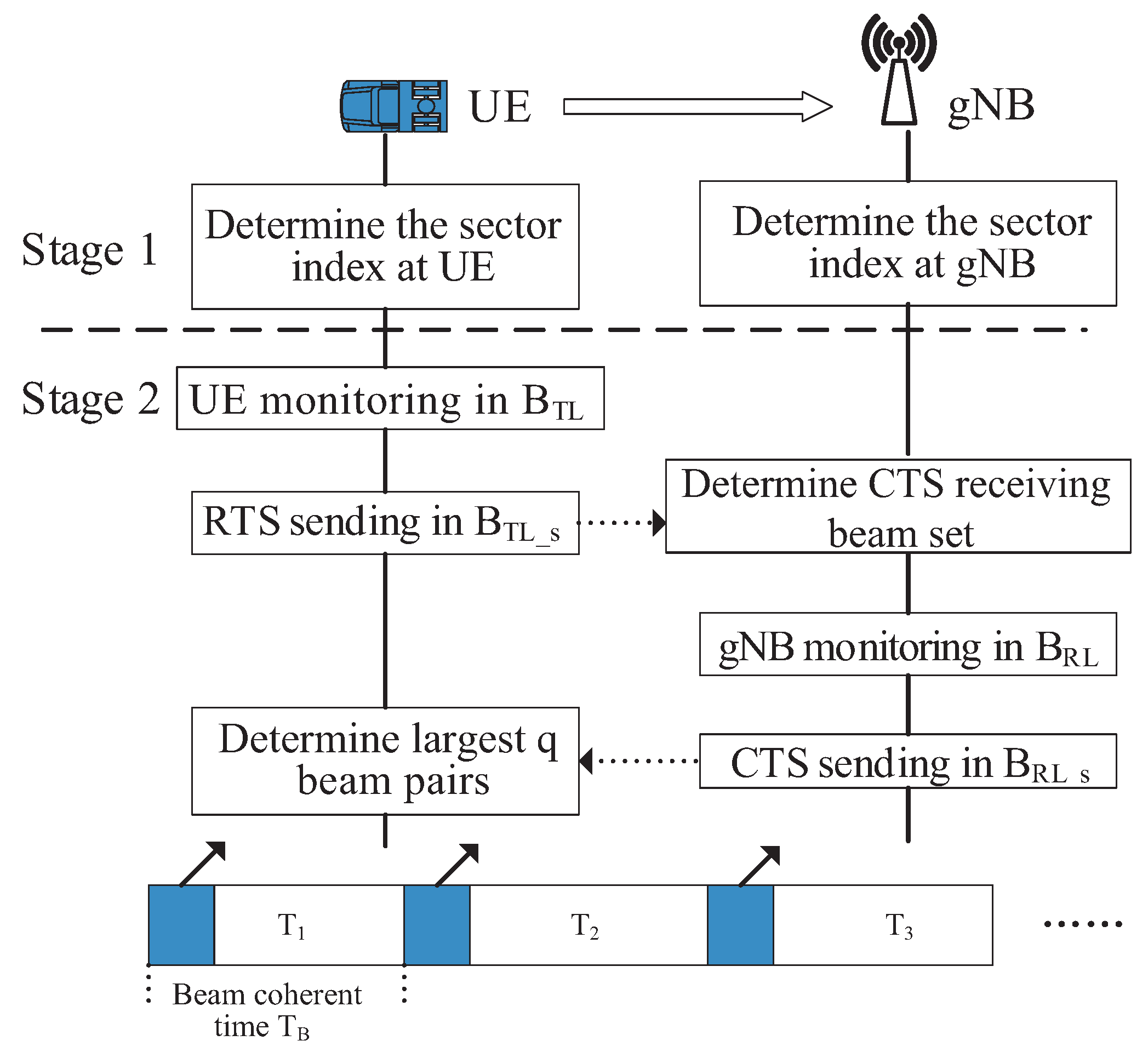
We divide the JDLBT into four stages: UE monitoring, RTS sending, gNB monitoring, and CTS sending. Based on channel reciprocity theory between uplink and downlink, the details are describe as follows.

4.2.1. UE Monitoring

The UE sweeps the beam set B T L = { T L 1 , T L 2 , , T L K 1 } which belongs to the selected sector according to the angle correlation and detects the channel energy on each beam direction. If the co-channel interference is lower than the CCA threshold β t h , the transmitter will choose these beams as a subset of B T L to send RTS in the next stage. The subset is denoted as B T L _ s .

4.2.2. RTS Sending

The UE sends RTS on each beam direction in B T L _ s . At the same time, the gNB carries out a sector beam sweeping during each beam transmission cycle. Based on sounding reference signal (SRS), the gNB sorts the reference signal receiving power (RSRP) of the receiving beams in descending order after K 1 times of beam sweeping. Then, the the largest p beam indices in RSRP are sent to UE and adopted as the CTS receiving beam set at UE.

4.2.3. gNB Monitoring

In a similar way, the gNB scans its monitoring beam set B R L = { R L 1 , R L 2 , , R L M 1 } in the corresponding receiving beam sector. Then, the gNB performs CCA detection on those beam direction to pick out a subset of B R L , which is used for CTS sending in the next stage, denoted as B R L _ s .

4.2.4. CTS Sending

At the end of the procedure, the gNB sends CTS by sweeping each beams in B R L _ s to occupy the channels. Meanwhile, the UE sweeps the largest p beams in RSRP which are selected by RTS sending stage in each beam transmission cycle. According to the RSRP, the transceiver determine the largest q beam pairs as the communication beam set. Further, the optimal beam pairs are chosen as the current communication beams. Finally, the UE will report the beam index to gNB.
It should be noticed that the exposed node problem and hidden node problem can be solved with the help of RTS/CTS in JDLBT [19]. The JDLBT enables exposed node to establish a communication link with limited interference, and prevents hidden node form the link by stop sending CTS on beams with strong interference. In conclusion, the JDLBT avoids duplicating beam sweeping in the process of directional LBT and succeeding beam training, and reduces the latency and signaling overhead significantly. The range of beam set is further reduced with the help of the directional LBT.
The procedure of the TCFBT scheme is summarized in Figure 5.

4.3. Complexity Analysis

We analyze the complexity of TCFBT scheme in each beam coherent time in this subsection. Taking IEEE 802.15.3c three-stage search algorithm as the baseline [8], which is much less complex than ergodic searching, the complexity of the independent beam searching is O ( N s + N r ) , and it needs extra O ( 2 ( N s + N r ) ) beam pair links in the RTS/CTS sending process. Moreover, it requires N s times channel monitoring at UE side and N r times channel monitoring in gNB before beam training. Therefore, the total complexity is less than or equal to O ( 4 ( N s + N r ) ) , which is relatively high for beam tracking with mobile users.
When channel monitoring combines with beam tracking, the complexity become much lower than the independent scheme. Thanks to the sector prediction algorithm, the beam training set is narrowed to K 1 at the UE and M 1 at the gNB. In the process of RTS sending, the beam pair links are O ( K 1 × M 1 ) times, while the complexity is O ( M 1 × p ) at CTS sending. As a result, the complexity of the proposed TCFBT scheme is O ( K 1 + M 1 + K 1 × M 1 + M 1 × p ) . As shown in Table 2, we assume there are eight sectors at the gNB and the size of alternative beam set p is equal to 3. The beam pair links are largely reduced by using TCFBT scheme.

5. Simulations Results

In this section, we evaluate the proposed TCFBT scheme with different beam coherent time in single link and validate the TCFBT scheme with newly derived beam coherent time for 5G communication systems at 60 GHz mmWave band. All evaluations use the mmWave eSV channel described in Section 2.2. We only consider LOS case here. When the locations of the users are determined, the AOA and AOD can be fixed correspondingly. The variety of channel is mainly caused by the mobility of UE and Doppler frequency shift. To calculate the overhead of signaling interaction, we employ the beam management scheme mentioned in Section 4.3. Define the signal power of the user i in each beam switching time as P i , T B . In addition, the analog beamforming vectors are generated by DFT codebooks in the following simulations. Assume each UE moves with a constant speed 1 m/s and the trajectory are generated by random walk model. The UE can choose a direction from nine candidates to move forward. Note that the coverage of gNB is limited to 100 m, and we do not consider the handover between gNB in this paper due to the small plant area. The simulation parameters are shown in Table 3.

5.1. The Performance of the TCFBT Scheme with Different Beam Coherent Time

We analyze the effectiveness in multi-user single links communication scenario, where N s = 16 and N r = 64 . Three metrics are defined to evaluate the performance of the proposed TCFBT scheme with different beam coherent times, namely ergodic capacity, the effective ergodic capacity, and outage probability. We define the outage probability as P o u t = P { R i < R t h } , where R i is the instantaneous spectrum efficiency of user i, R t h is the outage threshold, and P { } represents the probability of interruption. The threshold of beam misalignment ξ t h is set to 0.5. Then, the proposed TCFBT scheme with two newly derived beam coherence times is compared with channel coherence time defined in [10] and beam coherence time presented in [16].
Referring to single user MIMO, the ergodic capacity with different beam coherent times is shown in Figure 6. The channel coherence time presented in [10] has the highest ergodic capacity than the proposed two beam coherent time. Compared with beam coherent time derived by von Mises [16], the FET fitting declines approximately 40 % . The ergodic capacity of TGF fitting is five times higher than the von Mises fitting when SNR=10. However, the duration of channel coherence time is much shorter than the proposed beam coherent time, which will bring more latency and signal interaction. To further illustrate the effect of overhead, we compare the effective ergodic capacity of the proposed beam coherent time.
As shown in Figure 7, the TGF fitting has the highest effective ergodic capacity, followed by the other beam coherent time. Because of frequent switching, the effective ergodic capacity of channel coherence time declines about 30 % compared with the ergodic capacity in Figure 6. Since the beam coherent time derived by von Mises is much longer and less accurate than the proposed beam coherent time, the effective ergodic capacity is lower than that of TGF fitting and FET fitting. Actually, FET is more adapted to fitting coarse beam where its beamwidth is greater than or equal to π / 3 . Therefore, the effective ergodic capacities of FET and von Mises are still much lower than that of TGF fitting when N s = 16 and N r = 64 .
In Figure 8, the solid lines represent the outage threshold equals to 1 bit/s/Hz with N s = 16 , N r = 64 , and the antenna beamwidth is fine, and the dash lines are the outage probabilities with the same outage threshold where the beamwidth is coarse, N s = 4 , and N r = 16 . Due to the frequent switching, the channel coherent time has the lowest outage probability both in fine beams and in coarse beams. With less switching latency, the outage probability of TGF fitting is slightly higher than the beam coherence time at lower SNRs, while the gap become smaller with the increasing of SNR. This observation demonstrates frequent beam switching does maintain the communication links. However, the beam coherent time with TGF fitting can reduce delay and signaling overhead in a large extent. It should be noticed that the beam coherent times derived by FET and von Mises fitting have higher outage probabilities. As the number of antennas increases, the gap between TGF and FET fitting grows. It indicates that the FET fitting is more suitable for coarse beam, while this beam coherent time is relatively longer for fine beams.
Figure 9 depicts the optimal beam searching time T s setting for the proposed TCFBT scheme with the increasing complexity. It should be noticed that the complexity in our simulation consists of two parts: one is the number of beam pair links which influence the beam searching time T s and the other is the number of antennas at transceiver which influence the computation complexity. Consequently, Figure 9 shows the simulation results in these two parts. Firstly, it can be observed that the effective ergodic capacity increases with the growing of T s and tends to flatten when T s is longer enough to find the optimal beam pairs. Secondly, as the number of antennas increases, a longer beam search time is required to achieve the maximum effective ergodic capacity. Therefore, the optimal beam searching times T s for TCFBT scheme with different numbers of antennas are the inflection points of each curve in the figure.

5.2. The Performance of the TCFBT Scheme with Newly Derived Beam Coherent Time

To validate the performance of the proposed TCFBT scheme with newly derived beam coherent time at 60 GHz mmWave spectrum, we adopt the system model described in Section 2.1. Assume that there are eight 5G users communicating with the corresponding gNBs. We adopt the the beam coherent time derived by TGF fitting here. The threshold of beam misalignment ξ t h is set to 0.5, while the CCA threshold β t h is defined as 0.5 times of signal power P i , T B for user i during each beam switching time.
As shown in Figure 10, the position prediction accuracy error has less effect on the effective ergodic capacity of the proposed TCFBT scheme compared with the fast beam tracking scheme in [10]. The Gaussian process-based sector prediction algorithm only confirms a sector range from eight determined sector rather than a certain beam direction on the transceiver. Then, the JDLBT algorithm will adopt to obtain the optimal beam pairs. Therefore, if the position prediction accuracy error is less than π / 4 degrees, the effective ergodic capacity of the proposed algorithm will not be affected.
Figure 11 illustrates the effectiveness of the TCFBT scheme with TGF fitting in terms of effective ergodic capacity of the communication networks. We can observe that the effective ergodic capacity of the proposed scheme is far superior to that of the fast beam tracking scheme proposed in [10] under common beam coherent time with the same position prediction algorithm. There are two reasons for this trend. Firstly, directional LBT helps the transceiver avoiding some beam directions to form the communication links according to CCA threshold, which reduces the effect of interference. Secondly, the proposed scheme requires less position prediction accuracy than the beam tracking scheme in [10]. Therefore, the proposed TCFBT scheme can reduce the influence of position noise in Gaussian process-based sector prediction.
In Figure 12, we show the average latency of the proposed scheme with TGF fitting in terms of the number of antennas. Each transceiver is divided into eight sectors, which are used for determine the subset in the first stage during the Gaussian positioning process. With the position prediction and directional LBT, the TCFBT scheme we propose has the lowest latency, which ensures the efficiency of beam tracking of mobile terminal in massive MIMO system.
Figure 13 depicts the relationship between the effective ergodic capacity and the number of 5G communication links. Due to the interference between users, the effective ergodic capacity does not increase linearly as the number of communication links increases. Compared with the fast beam tracking scheme in [10], directional LBT in the proposed scheme avoids the beam direction with strong interference due to the CCA threshold, and ensures the reliability of the formed communication links. Therefore, higher effective ergodic capacity and the near optimal beam pairs can be achieved by the proposed scheme.

6. Conclusions

In this paper, we propose a two-stage TCFBT scheme to reduce the latency and signaling overhead in the process of beam tracking, while avoiding the beam direction with strong interference from other moving terminals according CCA threshold in 5G wireless communication networks. We determine the optimal beam pairs and maintain the communication links during each beam coherent time. The numerical results show that the beam coherent time is much longer than the channel coherent time. The performance of TGF fitting outperforms the other fitting function for DFT codebook when the number of antenna increases. Therefore, the two-stage TCFBT scheme we propose will greatly decrease the beam searching complexity in 5G system when the user moves.

Author Contributions

Conceptualization, P.L.; Data curation, P.L. and D.L.; Formal analysis, P.L. and D.L.; Funding acquisition, X.H. and J.W.; Methodology, D.L.; Software, P.L.; Writing—original draft, P.L.; and Writing—review and editing, D.L., P.L., and J.W. All authors have read and agreed to the published version of the manuscript.

Funding

This work is supported by Docomo Beijing Lab. This work is also supported in part by the National Natural Science Foundation of China under Grant No.61971069, 61801051, Key R&D Program Projects in Shanxi Province under Grant No. 2019ZDLGY07-10, and the Open Project of A Laboratory under Grant 2017XXAQ08.

Conflicts of Interest

The authors declare no conflict of interest.

Appendix A. Proof of Beam Coherence Time

Taking Fourier expansion fitting function as an example, we have
ξ t h = a 0 + a 1 cos ( w ( θ + Δ θ ) ) + b 1 sin ( w ( θ + Δ θ ) ) a 0 + a 1 cos ( w θ ) + b 1 sin ( w θ )
In light of trigonometric theorem, we obtain
a 0 ( 1 ξ t h ) + ( a 1 cos ( w θ ) + b 1 sin ( w θ ) ) ( cos ( w Δ θ ) ξ t h ) + ( b 1 cos ( w θ ) a 1 sin ( w θ ) ) sin ( w Δ θ ) = 0
When the angle Δ θ is small, the sin ( w Δ θ ) w Δ θ and cos ( w Δ θ ) 1 , it can be seen that
Δ θ = a 0 + a 1 cos ( w θ ) + b 1 sin ( w θ ) ( a 1 sin ( w θ ) b 1 cos ( w θ ) w
Combining Equation (9), we have derived the closed-form expression for beam coherence time (12). Similarly, the beam coherence time can be calculated by two-terms Gaussian function.

References

  1. Ma, Z.; Xiao, M.; Xiao, Y.; Pang, Z.; Poor, H.V.; Vucetic, B. High-Reliability and Low-Latency Wireless Communication for Internet of Things: Challenges, Fundamentals, and Enabling Technologies. IEEE Internet Things J. 2019, 6, 7946–7970. [Google Scholar] [CrossRef]
  2. Lu, X.; Sopin, E.; Petrov, V.; Galinina, O.; Moltchanov, D.; Ageev, K.; Andreev, S.; Koucheryavy, Y.; Samouylov, K.; Dohler, M. Integrated Use of Licensed- and Unlicensed-Band mmWave Radio Technology in 5G and Beyond. IEEE Access 2019, 7, 24376–24391. [Google Scholar] [CrossRef]
  3. Wang, X.; Kong, L.; Kong, F.; Qiu, F.; Xia, M.; Arnon, S.; Chen, G. Millimeter Wave Communication: A Comprehensive Survey. IEEE Commun. Surv. Tutor. 2018, 20, 1616–1653. [Google Scholar] [CrossRef]
  4. Liu, P.; Blumenstein, J.; Perovic, N.S.; di Renzo, M.; Springer, A. Performance of Generalized Spatial Modulation MIMO Over Measured 60 GHz Indoor Channels. IEEE Trans. Commun. 2018, 66, 133–148. [Google Scholar] [CrossRef]
  5. Ahmed, I.; Khammari, H.; Shahid, A.; Musa, A.; Kim, K.S.; De Poorter, E.; Moerman, I. A Survey on Hybrid Beamforming Techniques in 5G: Architecture and System Model Perspectives. IEEE Commun. Surv. Tutor. 2018, 20, 3060–3097. [Google Scholar] [CrossRef] [Green Version]
  6. Giordani, M.; Polese, M.; Roy, A.; Castor, D.; Zorzi, M. A Tutorial on Beam Management for 3GPP NR at mmWave Frequencies. IEEE Commun. Surv. Tutor. 2019, 21, 173–196. [Google Scholar] [CrossRef] [Green Version]
  7. Zhang, J.; Huang, Y.; Shi, Q.; Wang, J.; Yang, L. Codebook Design for Beam Alignment in Millimeter Wave Communication Systems. IEEE Trans. Commun. 2017, 65, 4980–4995. [Google Scholar] [CrossRef]
  8. Wang, J.; Lan, Z.; Pyo, C.-W.; Baykas, T.; Sum, C.-S.; Rahman, M.A.; Gao, J.; Funada, R.; Kojima, F.; Harada, H.; et al. Beam codebook based beamforming protocol for multi-Gbps millimeter-wave WPAN systems. IEEE J. Sel. Areas Commun. 2009, 27, 1390–1399. [Google Scholar] [CrossRef]
  9. Va, V.; Choi, J.; Shimizu, T.; Bansal, G.; Heath, R.W. Inverse Multipath Fingerprinting for Millimeter Wave V2I Beam Alignment. IEEE Trans. Veh. Technol. 2018, 67, 4042–4058. [Google Scholar] [CrossRef] [Green Version]
  10. Zhang, J.; Xu, W.; Gao, H.; Pan, M.; Feng, Z.; Han, Z. Position Prediction Based Fast Beam Tracking Scheme for Multi-User UAV-mmWave Communications. In Proceedings of the ICC 2019—2019 IEEE International Conference on Communications (ICC), Shanghai, China, 20–24 May 2019; pp. 1–7. [Google Scholar]
  11. Zhang, J.; Xu, W.; Gao, H.; Pan, M.; Feng, Z.; Han, Z. Position-Attitude Prediction Based Beam Tracking for UAV mmWave Communications. In Proceedings of the ICC 2019—2019 IEEE International Conference on Communications (ICC), Shanghai, China, 20–24 May 2019; pp. 1–7. [Google Scholar]
  12. Talvitie, J.; Levanen, T.; Koivisto, M.; Ihalainen, T.; Pajukoski, K.; Renfors, M.; Valkama, M. Positioning and Location-Based Beamforming for High Speed Trains in 5G NR Networks. In Proceedings of the 2018 IEEE Globecom Workshops (GC Wkshps), Abu Dhabi, UAE, 9–13 December 2018; pp. 1–7. [Google Scholar]
  13. Bao, J.; Li, H. Motion Aware Beam Tracking in Mobile Millimeter Wave Communications: A Data-Driven approach. In Proceedings of the ICC 2019—2019 IEEE International Conference on Communications (ICC), Shanghai, China, 20–24 May 2019; pp. 1–6. [Google Scholar]
  14. Koivisto, M.; Hakkarainen, A.; Costa, M.; Kela, P.; Leppanen, K.; Valkama, M. High-Efficiency Device Positioning and Location-Aware Communications in Dense 5G Networks. IEEE Commun. Mag. 2017, 55, 188–195. [Google Scholar] [CrossRef] [Green Version]
  15. Li, J.; Ai, B.; He, R.; Yang, M.; Wang, Q.; Zhang, B.; Zhong, Z. ClusterBased 3-D Channel Modeling for Massive MIMO in Subway Station Environment. IEEE Access 2018, 6, 6257–6272. [Google Scholar] [CrossRef]
  16. Va, V.; Choi, J.; Heath, R.W. The Impact of Beamwidth on Temporal Channel Variation in Vehicular Channels and Its Implications. IEEE Trans. Veh. Technol. 2017, 66, 5014–5029. [Google Scholar] [CrossRef]
  17. Gao, X.; Dai, L.; Yuen, C.; Wang, Z. Turbo-Like Beamforming Based on Tabu Search Algorithm for Millimeter- Wave Massive MIMO Systems. IEEE Trans. Veh. Technol. 2016, 65, 5731–5737. [Google Scholar] [CrossRef]
  18. Rasmussen, C.E.; Williams, C.I.K. Gaussian Processes for Machine Learning; MIT Press: Cambridge, MA, USA, 2006. [Google Scholar]
  19. Li, P.; Liu, D.; Yu, F. Joint Directional LBT and Beam Training for Channel Access in Unlicensed 60 GHz mmWave. In Proceedings of the 2018 IEEE Globecom Workshops (GC Wkshps), Abu Dhabi, UAE, 9–13 December 2018; pp. 1–6. [Google Scholar]
Figure 1. Multi-user single links in mobility scenario.
Electronics 09 00747 g001
Figure 2. Signal transmission model with analog beamforming structure.
Electronics 09 00747 g002
Figure 3. Motion model in two dimensional plane.
Electronics 09 00747 g003
Figure 4. Fitting of beam radiation pattern.
Electronics 09 00747 g004
Figure 5. The procedure of trajectory prediction and channel monitoring aided fast beam tracking scheme.
Electronics 09 00747 g005
Figure 6. The ergodic capacity vs. SNR with v = 1 m/s.
Electronics 09 00747 g006
Figure 7. The effective ergodic capacity vs. SNR with v = 1 m/s and OFDM duration = 8.92 u s .
Electronics 09 00747 g007
Figure 8. The outage probability vs. SNR with v = 1m/s.
Electronics 09 00747 g008
Figure 9. The effective ergodic capacity vs. T s with the proposed TCFBT scheme.
Electronics 09 00747 g009
Figure 10. The effective ergodic capacity vs. position prediction accuracy error.
Electronics 09 00747 g010
Figure 11. The effective ergodic capacity vs. SNR.
Electronics 09 00747 g011
Figure 12. The average latency vs. different antenna numbers.
Electronics 09 00747 g012
Figure 13. The effective ergodic capacity vs. different 5G communication links.
Electronics 09 00747 g013
Table 1. Symbol table.
SymbolsMeaning
A Matrix
a vector
a scalar
E [ x ] The expectation of the variable x
C N ( 0 , δ 2 ) Complex Gaussian distribution with zero mean and δ 2 variance
| | A | | F Frobenius norm
H Conjugate transpose of a matrix or vector
T Transpose of a matrix or vector
Table 2. The complexity of beam pair links.
UE Antenna = 2
gNB Antenna = 8
UE Antenna = 4
gNB Antenna = 16
UE Antenna = 16
gNB Antenna = 64
UE Antenna = 32
gNB Antenna = 128
3c searching<40<80<320<640
TCFBT scheme
(with 8 sector in gNB, p = 3)

<8

<20

<176

<608
Table 3. Simulation parameters.
ParametersValue
Simulation time5000 ms
Channel modeleSV
RayLOS
UE’s speed1 m/s
Maximum Doppler shift200 Hz
Motion ModelRandom walk
Channel coherent time5 ms
Number of antenna N s = 16 , N r = 64
Beam misalignment threshold ξ t h 0.5
CCA threshold β t h P i , T B / 2
Outage threshold R t h 1 bit/s/Hz
Noise variance in Gaussian process0.5

