Abstract
A knowledge graph (KG), also known as a knowledge base, is a particular kind of network structure in which the node indicates entity and the edge represent relation. However, with the explosion of network volume, the problem of data sparsity that causes large-scale KG systems to calculate and manage difficultly has become more significant. For alleviating the issue, knowledge graph embedding is proposed to embed entities and relations in a KG to a low-, dense and continuous feature space, and endow the yield model with abilities of knowledge inference and fusion. In recent years, many researchers have poured much attention in this approach, and we will systematically introduce the existing state-of-the-art approaches and a variety of applications that benefit from these methods in this paper. In addition, we discuss future prospects for the development of techniques and application trends. Specifically, we first introduce the embedding models that only leverage the information of observed triplets in the KG. We illustrate the overall framework and specific idea and compare the advantages and disadvantages of such approaches. Next, we introduce the advanced models that utilize additional semantic information to improve the performance of the original methods. We divide the additional information into two categories, including textual descriptions and relation paths. The extension approaches in each category are described, following the same classification criteria as those defined for the triplet fact-based models. We then describe two experiments for comparing the performance of listed methods and mention some broader domain tasks such as question answering, recommender systems, and so forth. Finally, we collect several hurdles that need to be overcome and provide a few future research directions for knowledge graph embedding.
1. Introduction
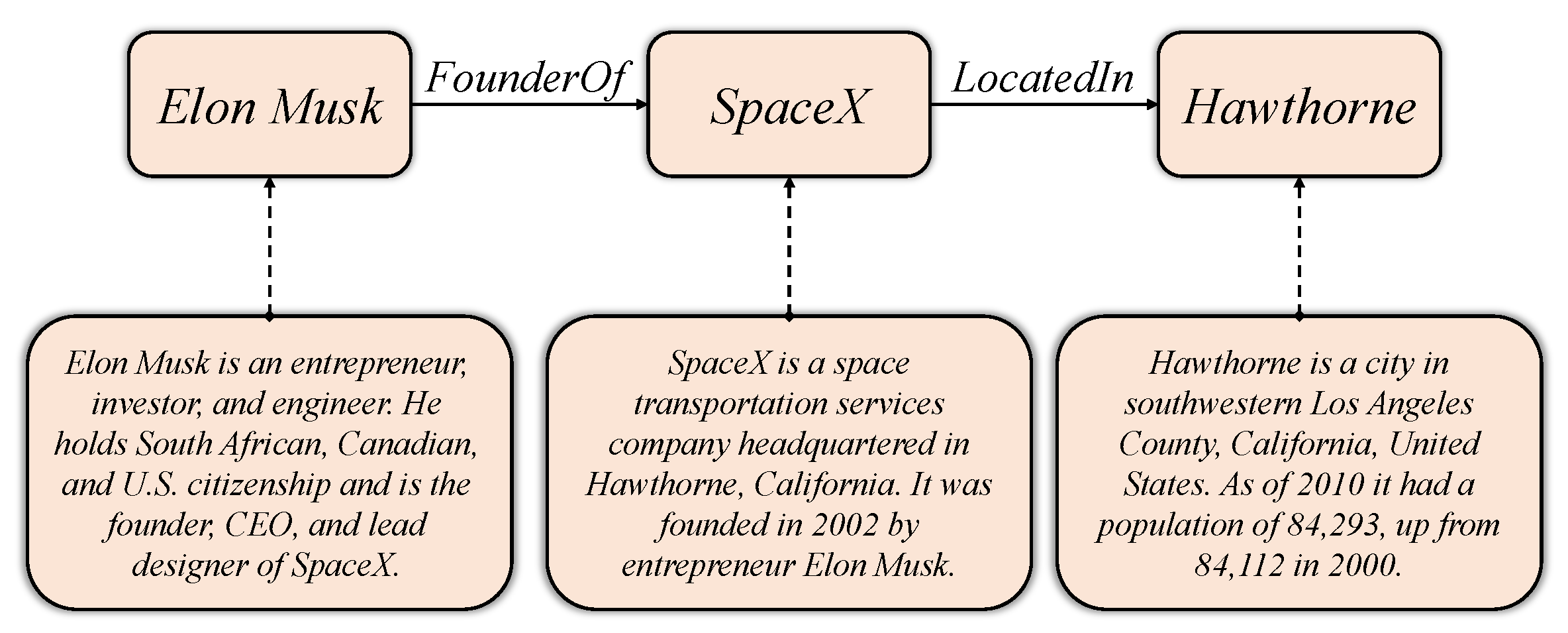
Numerous large-scale knowledge graphs, such as SUMO [1], YAGO [2], Freebase [3], Wikidata [4], and DBpedia [5], have been released in recent years. These KGs have become a significant resource for many natural language processing (NLP) applications, from named entity recognition [6,7] and entity disambiguation [8,9] to question answering [10,11] and information extraction [12,13]. In addition, as an applied technology, a knowledge graph also supports specific applications in many industries. For instance, it can provide visual knowledge representation for drug analysis, disease diagnosis in the field of medicine [14,15]; in the field of e-commerce, it can be used to construct a product knowledge graph to accurately match the user’s purchase intention and product candidate set [16,17]; it also can be employed in public security to analyze the relations between entities and obtain clues [18]. The knowledge graph stores real-world objective information that the data structure is in RDF-style triplets (http://www.w3.org/TR/rdf11-concepts/) , where h and t are head and tail entity, respectively, and r represents a relation between h and t. For instance, Figure 1 shows two triplets that each entity has a corresponding description. However, with the explosion of network volume, this traditional graph structure usually makes KGs hard to manipulate. The drawback of traditional KGs mainly includes the following two aspects: (i) Computational efficiency issues. When using the knowledge graph to calculate the semantic relations between entities, it is often necessary to design a special graph algorithm to achieve it. However, this graph algorithm has high computational complexity and poor scalability. While the knowledge graph reaches a large scale, it is difficult to meet the needs of real-time computing. (ii) Data sparsity problem. Similar to other large-scale data, the large-scale knowledge graph is also faced with a serious problem of data sparsity, which makes the calculation of semantic or inferential relations of entities extremely inaccurate.
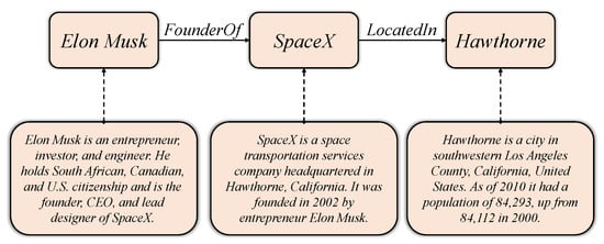
Figure 1.
A simple instance of a knowledge graph.
For tackling these challenge, knowledge graph embedding has been provided and attracted much attention, as it has the capability of knowledge graph to a dense and low dimensional, feature space [19,20,21,22,23,24,25] and it can efficiently calculate the semantic relation between entities in low dimensional space and effectively solve the problems of computational complexity and data sparsity. This method can further be used to explore new knowledge from existing facts (link prediction [19,23]), disambiguate entities (entity resolution [22,24]), extract relations (relation classification [26,27]), etc. The embedding procedure is described as follows. Given a KG, the entities and relations are first randomly represented in a low-, vector space, and an evaluation function is defined to measure the plausibility of each fact triplet. At each iteration, the embedding vectors of entities and relations can then be updated by maximizing the global plausibility of facts with some optimization algorithm. Even though there are a large number of successful researches in modeling relational facts, most of them can only train an embedding model on an observed triplets dataset. Thereupon, there are increasing studies that focus on learning more generalizing KG embedding models by absorbing additional information, such as entity types [28,29], relation paths [30,31,32], and textual descriptions [33,34,35].
Generally, knowledge graph embedding can utilize a distributed representation technology to alleviate the issue of data sparsity and computational inefficiency. This approach has three crucial advantages.
- The data sparsity problem has been effectively mitigated, because all elements in KGs including entities and relations are embedded to a continuous low-, feature space.
- Compared with traditional one-hot representation, KG embedding employs a distributed representation method to transform the original KG. As a result, it is effective to improve the efficiency of semantic computing.
- Representation learning uses a unified feature space to connect heterogeneous objects to each other, thereby achieving fusion and calculation between different types of information.
In this paper, we provide a detailed analysis of the current KG embedding technologies and applications. We systematically describe how the existing techniques address data sparsity and computation inefficiency problems, including the thoughts and technical solutions offered by the respective researchers. Furthermore, we introduce a wide variety of applications that benefit from KG embedding. Although a few surveys about KG representation learning have been published [36,37], we focus on a different aspect compared with these articles. Cai et al. [36] performed a survey of graph embedding, including homogeneous graphs [38,39,40], heterogeneous graphs [41,42,43], graphs with auxiliary information [28,44,45], and graphs constructed from non-relational data [46,47,48]. Compared with their work, we focus more specifically on KG embedding, which falls under heterogeneous graphs. In contrast to the survey completed by Wang et al. [37], we describe various applications to which KG embedding applies and compare the performance of the methods in these applications.
The rest of this article is organized as follows. In Section 2, we introduce the basic symbols and formal problem definition of knowledge graph embedding and discuss embedding techniques. We illustrate the general framework and training process of the model. In Section 3, we will explore the applications supported by KG embedding, and then compare the performance of the above representation learning model in the same application. Finally, we present our conclusions in Section 4 and look forward to future research directions.
2. Knowledge Graph Embedding Models
In this section, we firstly declare some notations and their corresponding explanations that will be applied in the rest of this paper. Afterward, we supply a general definition of the knowledge graph representation learning problem. Detailed explanations of notations are elucidated in Table 1.

Table 1.
Detailed explanation of notations.
2.1. Notation and Problem Definition
Problem 1.
Knowledge graph embedding:Given a KG composed of a collection of triplet facts , and a pre-defined dimension of embedding space d (To simplify the problem, we transform entities and relations into the uniform embedding space, i.e., ), KG embedding aims to represent each entity and relation into a d-, continuous vector space, where and indicate the set of entities and relations, respectively. In other words, a KG is represented as a set of d-, vectors, which can capture information of the graph, in order to simplify computations on the KG.
Knowledge graph embedding aims to map a KG into a dense, low-, feature space, which is capable of preserving as much structure and property information of the graph as possible and aiding in calculations of the entities and relations. In recent years, it has become a research hotspot, and many researchers have put forward a variety of models. The differences between the various embedding algorithms are related to three aspects: (i) how they represent entities and relations, or in other words, how they define the representation form of entitles and relations, (ii) how they define the scoring function, and (iii) how they optimize the ranking criterion that maximizes the global plausibility of the existing triplets. The different models have different insights and approaches with respect to these aspects.
We have broadly classified these existing methods into two categories: triplet fact-based, representation learning models and description-based representation learning models. In this section, we first clarify the thought processes behind the algorithms in these two types of graph embedding models, as well as the procedures by which they solve the representation problem. After that, the training procedures for these models are discussed in detail. It is worth noting that due to study limitations, we can not enumerate all relevant knowledge graph embedding methods. Therefore, we only describe some representative, highly cited and code-implemented algorithms.
2.2. Triplet Fact-Based Representation Learning Models
Triplet fact-based embedding model treats the knowledge graph as a set of triplets containing all observed facts. In this section, we will introduce three groups of embedding models: translation-based models, tensor factorization-based models, and neural network-based models.
2.2.1. Translation-Based Models
Since Mikolov et al. [49,50] proposed a word embedding algorithm and its toolkit word2vec, the distributed representations learning has attracted more and more attention. Using that model, the authors found that there are interesting translation invariance phenomena in the word vector space. For example:
where is the vector of word w transformed by the word2vec model. This result means that the word representation model can capture some of the same implicit semantic relationship between the words “” (“”) and “” (“”). Mikolov et al. proved experimentally that the property of translation invariance exists widely in the semantic and syntactic relations of vocabulary.
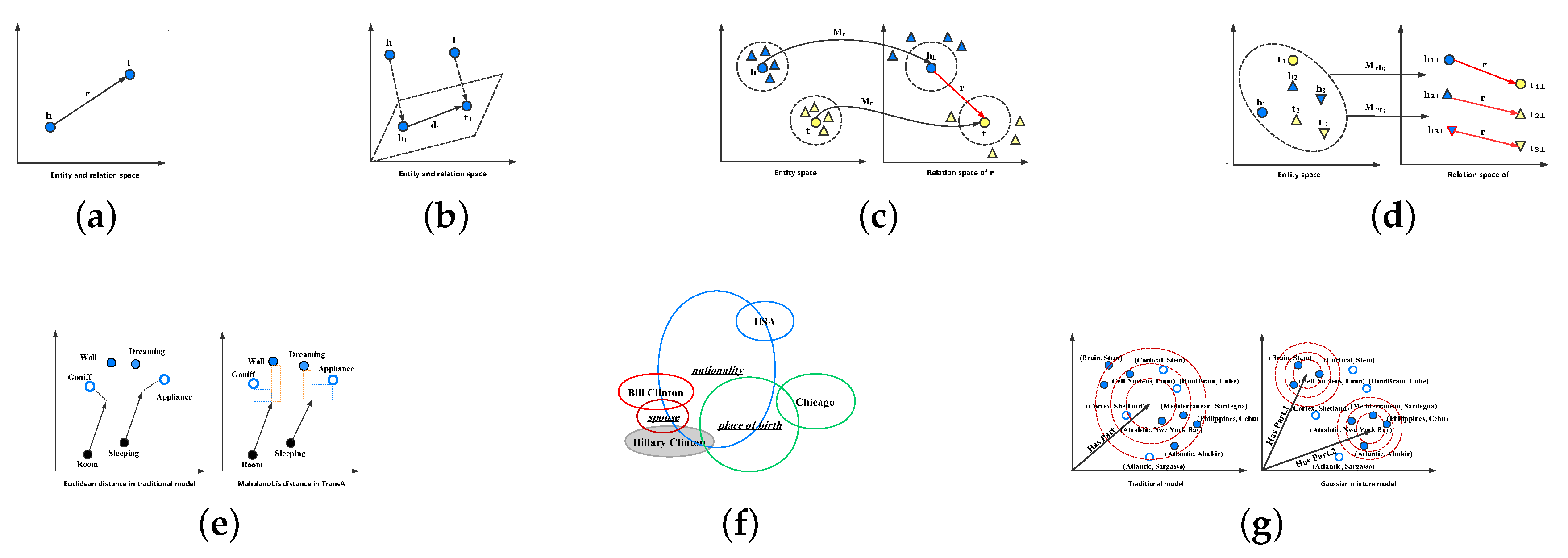
Inspired by the word2vec, Bordes et al. [19] introduced the idea of translation invariance into the knowledge graph embedding field, and proposed the TransE embedding model. TransE represents all entities and relations to the uniform continuous, low-, feature space , and the relations can be regarded as connection vectors between entities. Let E and R indicate the set of entity and relation, respectively. For each triplet (), the head and tail entity h, t, and the relation r are embedded to the embedding vectors , , and . As illustrated in Figure 2a, for each triplet (), TransE follows a geometric principle:
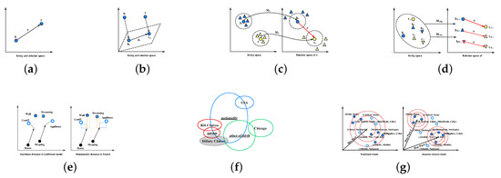
Figure 2.
Illustrations of translation-based models. (a) TransE, (b) TransH, (c) TransR, (d) TransD, (e) TransA, (f) KG2E, (g) TransG.
The authenticity of the given triplet () is computed via a score function. This score function is defined as a distant between and under -norm or -norm constraints. In mathematical expressions, it is shown as follows:
In order to learn an effective embedding model which has the ability to discriminate the authenticity of triplets, TransE minimizes a margin-based hinge ranking loss function over the training process.
where S and denote the set consisting of correct triplets and corrupted triplets, respectively, and indicates the margin hyperparameter. In training, TransE stochastically replaces the head or tail entity in each triplet with other candidate entities to generate corrupted triplet set . The construction formula is shown in Equation (5).
Although TransE has achieved a great advancement in large-scale knowledge graph embedding, it still has difficulty in dealing with complex relations, such as , , and [51,52]. For instance, there is a relation where the head entity has multiple corresponding tail entities, i.e., . According to the guidelines TransE followed , all embedding vectors of the tail entities should be approximately similar, as . More visually, there are two triplet facts and , in which is a relation mentioned above. Following TransE, the embedding vectors of and should be very similar in feature space. However, this result is clearly irrational because and are two companies in entirely different fields, except is their founder. In addition, other complex relations such as and also raise the same problem.
To handle this issue in complex relations, TransH [51] extended the original TransE model, it enables each entity to have different embedding representations when the entity is involved in diverse relations. In other words, TransH allows each relation to hold its own relation-specific hyperplane. Therefore, an entity would have different embedding vectors in different relation hyperplanes. As shown in Figure 2b, for a relation r, TransH employs the relation-specific translation vector and the normal vector of hyperplane to represent it. For each triplet fact , the embedding vectors of and are firstly projected to the relation-specific hyperplane in the direction of the normal vector . and indicate the projections.
Afterwards, the and are connected by the relation-specific translation vector . Similar to TransE, a small score is expected when holds. The score function is formulated as follows:
Here, is the squared Euclidean distance. By utilizing this relation-specific hyperplane, TransH can project an entity to different feature vectors depending on different relations, and solve the issue of complex relations.
Following this idea, TransR [52] extended on the original TransH algorithm. Although TransH enables each entity to obtain a different representation corresponding to its different relations, the entities and relations in this model are still represented in the same feature space . In fact, an entity may contain various semantic meanings and different relations may concentrate on entities’ diverse aspects; therefore, entities and relations in the same semantic space might make the model insufficient for graph embedding.
TransR expands the concept of relation-specific hyperplanes proposed by TransH to relation-specific spaces. In TransR, for each triplet , entities are embedded as and into an entity vector space , and relations are represented as a translation vector into a relation-specific space . As illustrated in Figure 2c, TransR projects and from the entity space into the relation space. This operation can render those entities (denoted as triangles with color) that are similar to head or tail entities (denoted as circles with color) in the entity space as distinctly divided in the relation space.
More specifically, for each relation r, TransR defines a projection matrix to transform the entity vectors into the relation-specific space. The projected entity vectors are signified by and , and the scoring function is similar to that of TransH:
Compared with TransE and TransH, TransR has made significant progress in performance. However, it also has some deficiencies: (i) For a relation r, the head and tail entities share the same projection matrix , whereas it is intuitive that the types or attributes between head and tail entities may be essentially different. For instance, in the triplet , is a person and is a company; they are two different types of entities. (ii) The projection from the entity space to the relation-specific space is an interactive process between entities and relations; it cannot capture integrated information when the projection matrix is generated only related to relations. (iii) Owing to the application of the projection matrix, TransR requires a large amount of computing resources, the memory complexity of which is , compared to TransE and TransH with .
To eliminate the above drawback, an improved method TransD [22] was proposed. It optimizes TransR by using two vectors for each entity-relation pair to construct a dynamic mapping matrix that could be a substitute for the projection matrix in TransR. Its illustration is in Figure 2d. Specifically, given a triplet , each entity and relation is represented to two embedding vectors. The first vector represents meanings of the entity/relation, denoted as , and , and the second vector (defined as , and ) is used to form two dynamic projection matrices . These two matrices are calculated as:
where is an identity matrix. Therefore, the projection matrix involve both entity and relation, and the embedding vectors of and are defined as:
Finally, the score function is the same as that of TransR in Equation (9). TransD refined this model, it constructs a dynamic mapping matrix with two projection vectors, that effectually reduces the computation complexity to .
All the methods described above including Trans (E, H, R, and D) ignore two properties of existing KGs: heterogeneity (some relations have many connections with entities and others do not), which causes underfitting on complex relations or overfitting on simple relations, and the imbalance (there is a great difference between head and tail entities for a relation in quantities), which indicates that the model should treat head and tail entities differently. TranSparse [24] overcomes the heterogeneity and imbalance by applying two model versions: TranSparse(share) and TranSparse(separate).
TranSparse (share) leverages adaptive sparse matrices to replace dense projection matrices for each relation r. The sparse degree is linked to the number of entities connected with relation r; it is defined as follows:
where () is a hyperparameter, denotes the number of entity pairs connected with the relation, and represents the maximum of them. Therefore, the projected vectors are formed by:
TranSparse (separate) employs two separate sparse mapping matrices, and , for each relation, where projects the head entities and the other projects the tail entities. The sparse degree and the projected vectors are extended as follows:
A simpler version of this method was proposed by Nguyen et al. [53], called sTransE. In that approach, the sparse projection matrices and are replaced by mapping matrices and , such that the projected vectors are transformed to:
The methods introduced so far merely modify the definition of the projection vectors or matrices, but they do not consider other aspects to optimize TransE. TransA [54] also boosted the performance of the embedding model from another view point by modifying the distance measure of the score function. It introduces adaptive Mahalanobis distance as a better indicator to replace the traditional Euclidean distance because Mahalanobis distance shows better adaptability and flexibility [55]. Given a triplet , is defined as a symmetric non-negative weight matrix with the relation r; the score function of TransA is formulated as:
As shown in Figure 2e, the two arrows represent the same relation , and and are true facts. If we use the isotropic Euclidean distance, which is utilized in traditional models to distinguish the authenticity of a triplet, it could yield erroneous triplets such as . Fortunately, TransA has the capability of discovering the true triplet via introducing the adaptive Mahalanobis distance because the true one has shorter distances in the x or y directions.
The above methods embedded the entity and relation to a real number space, KG2E [56] proposed a novel approach that introduces the uncertainty to construct a probabilistic knowledge graph embedding model. KG2E takes advantage of multi, Gaussian distributions to embed entities and relations; each entity and relation is represented to a Gaussian distribution, in which the mean of this Gaussian distribution is the position of the entity or relation in a semantic feature space, and the covariance signifies the uncertainty of the entity or relation, i.e.,
Here, are the mean vectors of , , and , respectively, and indicate the covariance matrices corresponding to entities and relations. KG2E also utilizes the distance between and as metric to distinguish the authenticity of triplets, where the traditional is transformed to the distribution formula of . This model employs two categories of approaches to estimate the similarity between two probability distributions: Kullback–Leibler divergence [57] and expected likelihood [58].
Figure 2f displays an illustration of KG2E. Each entity is represented as a circle without underline and the relations are the circles with underline. These circles with the same color indicate an observed triplet, where the head entity of all triplets is . The area of a circle denotes the uncertainty of the entity or relation. As we can see in Figure 2e that there are three triplets, and the uncertainty of the relation “” is lower than the others.
TransG [59] discusses the new situation of multiple relationship semantics, that is, when a relationship is associated with different entity pairs, it may contain multiple semantics. It also uses a Gaussian distribution to embed entities, but it is significantly different from KG2E because it leverages a Gaussian mixture model to represent relations:
where is the weight of distinct semantics and indicates an identity matrix. As shown in Figure 2g, dots are correct entities related to the relation “” and the triangles represent corrupted entities. In the traditional models (left), the corrupted entities do not have the ability to distinguish from the entire set of entities because all semantics are confused in the relation “.” In contrast, TransG (right) can find the incorrect entities by utilizing multiple semantic components.
TransE only has the ability to handle simple relations, and it is incompetent for complex relations. The extensions of TransE, including TransH, TransR, TransD, TransA, TransG, and so forth, proposed many thoughtful and insightful models to address the issue of complex relations. Extensive experiments in public benchmark datasets, which are generated from WordNet [60] and Freebase, show that these modified models achieve significant improvements with respect to the baseline, and verify the feasibility and validity of these methods. A comparison of these models in terms of their scoring functions and space size is shown in Table 2.

Table 2.
Comparison of translation-based models in terms of scoring functions and memory complexity. In KG2E, and ; m indicates the number of semantic components for each relation in TransG.
2.2.2. Tensor Factorization-Based Models
Tensor factorization is another category of effective methods for KG representation learning. The core idea of these methods is described as follows. First, the triplet facts in the KG are transformed into a 3D binary tensor . As illustrated in Figure 3, given a tensor , where n and m denote the number of entities and relations, respectively, each slice () corresponds to a relation type , and refers to the fact that the triplet (i-th entity, k-th relation, j-th entity) exists in the graph; otherwise, indicates a non-existent or unknown triplet. After that, the embedding matrices associated with the embedding vectors of the entities and relations are calculated to represent as some factors of a tensor. Finally, the low-, representation for each entity and relation is generated along with these embedding matrices.
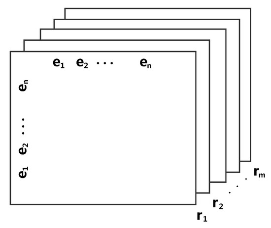
Figure 3.
A tensor model of knowledge graph.
RESCAL [61] applies a tensor to express the inherent structure of a KG and uses the rank-d factorization to obtain its latent semantics. The principle that this method follows is formulated as:
where is a matrix that captures the latent semantic representation of entities and is a matrix that models the pairwise interactions in the k-th relation. According to this principle, the scoring function for a triplet is defined as:
Here, , are the embedding vectors of entities in the graph and the matrix represents the latent semantic meanings in the relation. It is worth noting that and , which represent the embedding vectors of the i-th and j-th entity, are actually assigned by the values of the i-th and j-th row of matrix A in Equation (21). A more complex version of was proposed by García-Durán et al. [62], which extends RESCAL by introducing well-controlled two-way interactions into the scoring function.
However, this method requires parameters. To simplify the computational complexity of RESCAL, DistMult [63] restricts to be diagonal matrices, i.e., . The scoring function is transformed to:
DistMult not only reduces the algorithm complexity into , but the experimental results also indicate that this simple formulation achieves a remarkable improvement over the others.
Hole [64] introduced a circular correlation operation [65], denoted as , between head and tail entities to capture the compositional representations of pairwise entities. The formulation of this operation is shown as follows:
The circular correlation operation has the significant advantage that it can reduce the complexity of the composite representation compared to the tensor product. Moreover, its computational process can be accelerated via:
Here, indicates the fast Fourier transform (FFT) [66], denotes its inverse, and denotes the complex conjugate of . Thus, the scoring function corresponding to Hole is defined as:
It is noteworthy that circular correlation is not commutative, i.e., ; therefore, this property is indispensable for modeling asymmetric relations to semantic representation space.
The original DistMult model is symmetric in head and tail entities for every relation; Complex [67] leverages complex-valued embeddings to extend DistMult in asymmetric relations. The embeddings of entities and relations exist in the complex space , instead of the real space in which DistMult embedded. The scoring function is modified to:
where denotes the real part of a complex value, and represents the complex conjugate of . By using this scoring function, triplets that have asymmetric relations can obtain different scores depending on the sequences of entities.
In order to settle the independence issue of entity embedding vectors in Canonical Polyadic (CP) decomposition, SimplE [68] proposes a simple enhancement of CP which introduces the reverse of relations and computes the average CP score of and :
where ∘ is the element-wise multiplication and indicates the embedding vector of reverse relation. Inspired by Euler’s identity , RotatE [69] introduces the rotational Hadmard product, it regards the relation as a rotation between the head and tail entity in complex space. The score function is defined as follows:
QuatE [70] extends complex space into four-dimensional, hypercomplex space , it utilizes the Hamilton product to obtain latent inter-dependency between entities and relations in this complex space:
where ⊗ denotes the Hamilton product. Table 3 summarizes the scoring function and memory complexity for all tensor factorization-based models.

Table 3.
Comparison of tensor factorization-based models in terms of scoring functions and memory complexity.
2.2.3. Neural Network-Based Models
Deep learning is a very popular and extensively used tool in many different fields [71,72,73,74]. They are also models with strong representation and generalization capabilities that can express complicated nonlinear projections. In recent years, it has become a hot topic to embed a knowledge graph into a continuous feature space by a neural network.
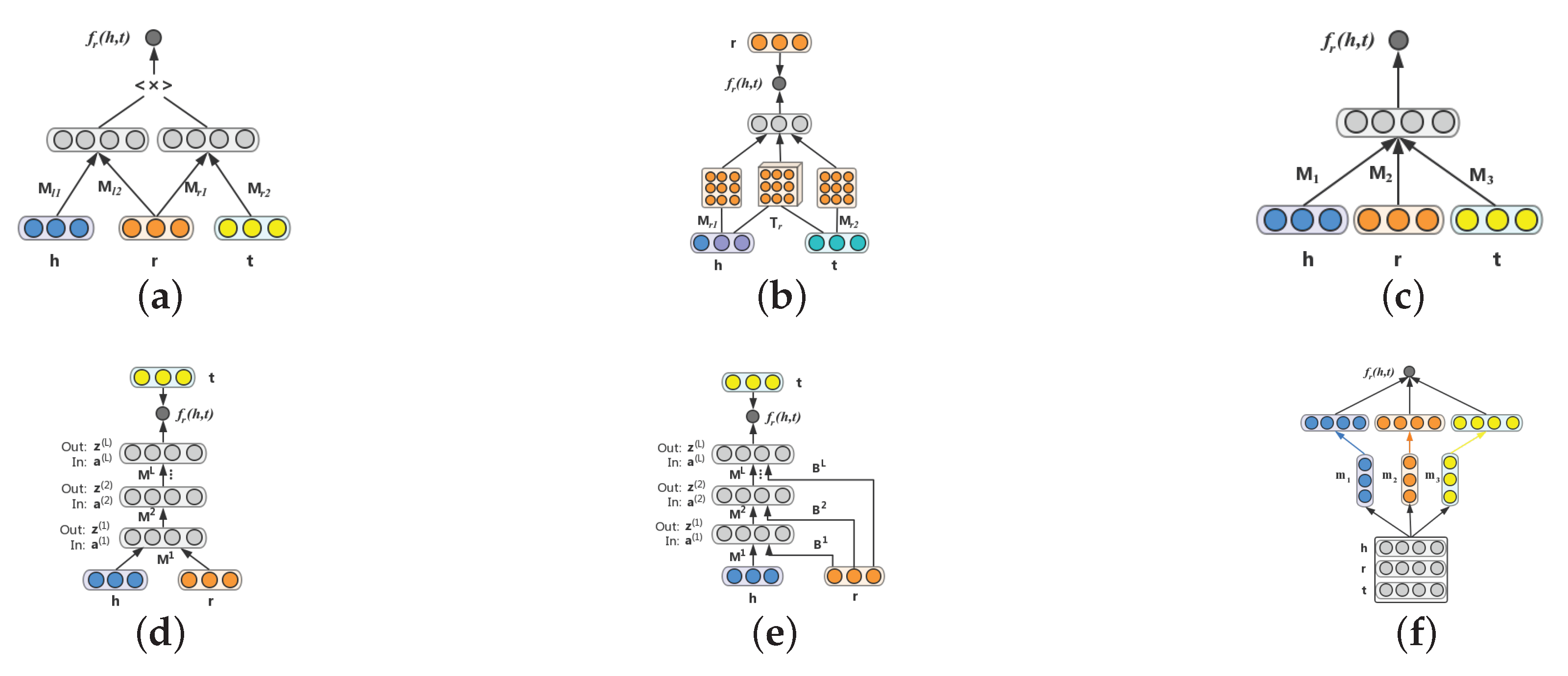
SME [21] defines an energy function for semantic matching, which can be used to measure the confidence of each observed fact by utilizing neural networks. As shown in Figure 4a, in SME, each entity and relation is firstly embedded to its embedding feature space. Then, to capture intrinsic connections between entities and relations, two projection matrices are applied. Finally, the semantic matching energy associated with each triplet is computed by a fully connected layer. More specifically, given a triplet in Figure 4a, SME represents entities and relations to the semantic feature space by the input layer. The head entity vector is then combined with the relation vector to acquire latent connections (i.e., ). Likewise, is generated from the tail entity and the relation vectors and . Bordes et al. provided two types of functions, so there are two versions for SME. SME is formulated by Equation (31):
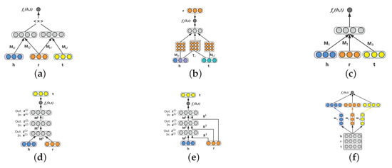
Figure 4.
Illustrations of neural network-based-based models. (a) SME, (b) NTN, (c) MLP, (d) NAM, (e) RMNN, (f) ConvKB.
SME (bilinear) is formulated in Equation (32):
where is the weight matrix and denotes the bias vector. Finally, the and are concatenated to obtain the energy score via a fully connected layer.
NTN [20] proposes a neural tensor network to calculate the energy score . It replaces the standard linear layer, which is in the traditional neural network, by employing a bilinear tensor layer. As shown in Figure 4b, given an observed triplet , the first layer firstly embeds entities to their embedding feature space. There are three inputs in the second nonlinear hidden layer including the head entity vector , the tail entity vector and a relation-specific tensor . The entity vectors , are embedded to a high-level representation via projection matrices respectively. These three elements are then fed to the nonlinear layer to combine semantic information. Finally, the energy score is obtained by providing a relation-specific linear layer as the output layer. The score function is defined as follows:
where indicates an activation function and denotes a bias, which belongs to a standard neural network layer. Meanwhile, a simpler version of this model is proposed in this paper, called a single layer model (SLM), as shown in Figure 4c. This is a special case of NTN, in which . The scoring function is simplified to the following form:
NTN requires a relation-specific tensor for each relation, such that the number of parameters in this model is huge and it would be impossible to apply to large-scale KGs. MLP [75] provides a lightweight architecture in which all relations share the same parameters. The entities and relation in a triplet fact are synchronously projected into the embedding space in the input layer, and they are involved in higher representation to score the plausibility by applying a nonlinear hidden layer. The scoring function is formulated as follows:
Here, is an activation function, and represent the mapping matrices that project the embedding vectors , and to the second layer; are the second layer parameters.
Since the emergence of deep learning technology, more and more studies have been proposed for deep neural networks (DNNs) [71,76,77]. NAM [78] establishes a deep neural network structure to represent a knowledge graph. As illustrated in Figure 4d, given a triplet , NAM firstly embeds each element in the triplet to embedding feature space. Then, the head entity vector and the relation vector are concatenated to a single vector as the input to feed to the layer where it consists of L rectified linear (ReLU) [79] hidden layers as follows:
where is the weight matrix and is the bias for layer ℓ. Finally, a score is calculated by applying the output pf the last hidden layer with the tail entity vector :
where is a sigmoid activation function. A more complicated model is proposed in this paper, called relation-modulated neural networks (RMNN). Figure 4e shows an illustration of this model. Compared with NAM, it generates a knowledge-specific connection (i.e., relation embedding ) to all hidden layers in the neural network. The layers are defined as follows:
where and denote the weight and bias matrices for layer ℓ, respectively. After the feed-forward process, RMNN can yield a final score using the last hidden layer’s output and the concatenation between the tail entity vector and relation vector :
ConvKB [80] captures latent semantic information in the triplets by introducing a convolutional neural network (CNN) for knowledge graph embedding. In the model, each triplet fact is represented to a three-row matrix, in which each element is transformed as a row vector. The matrix is fed to a convolution layer to yield multiple feature maps. These feature maps are then concatenated and projected to a score that is used to estimate the authenticity of the triplet via the dot product operation with the weight vector.
More specifically, as illustrated in Figure 4f, . First, the embedding vectors , , and are viewed as a matrix , and indicates the i-th column of matrix . After that, the filter is slid over the input matrix to explore the local features and obtain a feature map , such that:
where signifies the ReLU activation function and b indicates the bias. For this instance, there are three feature maps corresponding to three filters. Finally, these feature maps are concatenated as a representation vector , and calculated with a weight vector by a dot product operation. The scoring function is defined as follows:
Here, is the set of filters, and denotes that a convolution operation is applied to matrix via the filters in the set . is the concatenation operator. It is worth mentioning that and are shared parameters; they are generalized for all entities and relations.
In recent years, graph neural networks (GNNs) have captured more attention due to their great ability in representation of graph structure. R-GCN [81] is an improved model, which provides relation-specific transformation to represent knowledge graphs. The forward propagation is formulated as follows:
where signifies the hidden state of the entity i in l-th layer, indicates a neighbor collection where it connects to entity i with relation , and are the weight matrices, and denotes the normalization process such as .
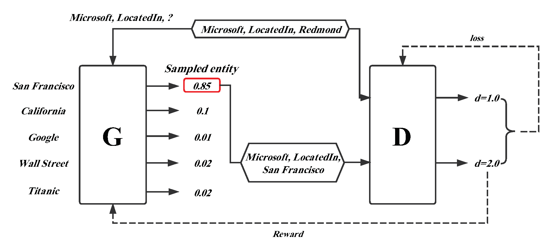
Inspired by burgeoning generative adversarial networks (GANs), Cai et al. [82] proposed a generative adversarial learning framework to improve the performance of the existing knowledge graph representation models and named it KBGAN. KBGAN’s innovative idea is to apply a KG embedding model as the generator to obtain plausible negative samples, and leverage the positive samples and generated negative samples to train the discriminator, which is the embedding model we desire.
A simple overview introducing the framework is shown in Figure 5. There is a ground truth triplet , which is corrupted by disposing of its tail entity, such as . The corrupted triplet is fed as an input into a generator (G) that can receive a probability distribution over the candidate negative triplets. Afterwards, the triplet with the highest probability is sampled as the output of the generator. The discriminator (D) utilizes the generated negative triplet and original truth triplet as input to train the model, and computes their score d, which indicates the plausibility of the triplet. The two dotted lines in the figure denote the error feedback in the generator and discriminator. One more point to note is that each triplet fact-based representation learning model mentioned above can be employed as the generator or discriminator in the KBGAN framework to improve the embedding performance. Table 4 illustrates the scoring function and memory complexity of each neural network-based model.
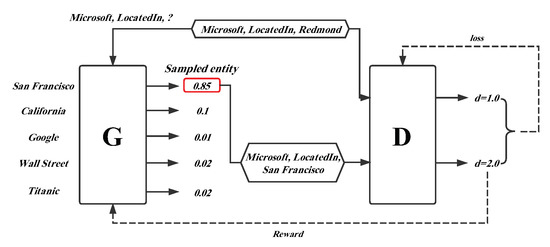
Figure 5.
Framework of the KBGAN model.

Table 4.
Comparison of neural network-based models in terms of scoring functions and memory complexity.
The above three types of triplet fact-based models focus on modifying the calculation formula of the scoring function , and their other routine training procedures are roughly uniform. The detailed optimization process is illustrated in Algorithm 1. First, all entity and relation embedding vectors are randomly initialized. In each iteration, a subset of triplets is constructed by sampling from the training set S, and it is fed into the model as inputs of the minibatch. For each triplet in , a corrupted triplet is generated by replacing the head or tail entity with other ones. After that, the original triplet set S and all generated corrupted triplets are incorporated as a batch training set . Finally, the parameters are updated by utilizing certain optimization methods.
Here, the set of corrupted triplets is generated according to , and there are two alternative versions of the loss function. The margin-based loss function is defined as follows:
and the logistic loss function is:
where is a margin hyperparameter and is a label that indicates the category (negative or positive) to which a given training triplet belongs. These two functions can both be calculated by the stochastic gradient descent (SGD) [83] or Adam [84] methods.
| Algorithm 1 Learning triplet fact-based models. |
| Input: The training set , entity set E, relation set R, embedding dimension k Output: Entity and relation embeddings
|
2.3. Description-Based Representation Learning Models
The models introduced above embed knowledge graphs to a specific feature space only based on triplets . In fact, a large number of additional information associated with knowledge graphs can be efficiently absorbed to further refine the embedding model’s performance, such as textual descriptions information and relation path information.
2.3.1. Textual Description-Based Models
Textual information falls into two categories: entity type information and descriptive information. The entity type specifies the semantic class to which the entity belongs. For example, belongs to category and belongs to . An entity description is a paragraph that describes the attributes and characteristics of an entity, for example, “Tesla, Inc. is an American electric vehicle and clean energy company with headquarters in Palo Alto, California”.
The textual description-based model is an extension of the traditional triplet-based model that integrates additional text information to evolve its performance. We introduce these models in an expanded order based on translation, tensor factorization, and neural network methods.
The extensions of translation-based methods. Xie et al. [85] proposed a novel type-embodied knowledge graph embedding learning method (TKRL) that exploits hierarchical entity types. It suggests that an entity may have multiple hierarchical types, and different hierarchical types should be transformed to different type-specific projection matrices.
In TKRL, for each fact , the entity embedding vectors and are first represented by using type-specific projection matrices. Let and denote the projected vectors:
where and indicate the projection matrices related to and . Finally, with a translation between two mapped entities, the scoring function is defined as the general form of the translation-based method:
To capture multiple-category semantic information in entities, the projection matrix / (we use to illustrate the approach) is generated as the weighted summation of all possible type matrices, i.e.,:
where n is the number of types to which the head entity belongs, indicates the i-th type, represents the projection matrix of , signifies the corresponding weight, and denotes the collection of types that the head entity can be connected to with a given relation r. To further mine the latent information stored in hierarchical categories, the matrix is designed by two types of operations:
where m is the number of subcategories for the parent category in the hierarchical structure, is the l-th subcategory, is the projection matrix corresponding to , and denotes the corresponding weight of .
TKRL introduces the entity type to enhance the embedding models; another aspect of textual information is entity description. Wang et al. [86] proposed a text-enhanced knowledge graph embedding model, named TEKE, which is also an extension of translation-based models.
Given a knowledge graph, TEKE firstly builds an entity description text corpus by utilizing an entity linking tool, i.e., AIDA [87] for annotating all entities, then constructs a co-occurrence network that has the ability of calculating the frequency of co-occurrence with the entities and words. This paper advised that the rich textual information of adjacent words can effectively represent a knowledge graph. Therefore, given an entity e, the model defines the valid textual context to become its neighbors, and pairwise textual context as common neighbors between the head and tail entity for each relation r.
Then, the pointwise textual context embedding vector is obtained through the word embedding toolkit. The pairwise textual context vector is a yield following a similar way. Finally, these feature vectors that capture the textual information are employed to calculate the score, such as TransE:
where and denote the weight matrices, , , and are the bias vectors. The score function is formulated as follows:
The extensions of tensor factorization-based methods. Apart from taking advantage of triplet information, Krompaß et al. [88] proposed an improved representation learning model for tensor factorization-based methods. It integrates prior type-constraint knowledge with triplet facts in original models, such as RESCAL, and achieves impressive performance in link prediction tasks.
Entities in large-scale KGs generally have one or multifarious predefined types. The types of head and tail entities in a specific relation are constrained, which refers to type-constraints. For instance, the relation is reasonably only appropriate for the , to which the head and tail entities belong. In this model, , as an indication vector, denotes the head entity types that satisfy the type-constraints of relation k; is also an indication vector index for the tail entity constraints of relation k.
The main difference between this model and RESCAL is that the novel model indexes only those latent embeddings of entities related to the relation type k, compared with indexing the whole matrix A, as shown in Equation (21), in RESCAL.
Here, indicates the indexing of rows from the matrix A, and is the indexing of . As a result of its simplification, this model shows a shorter iteration time and it is more suitable for large-scale KGs.
The extensions of neural network-based methods. The detailed description information associated with entities and relations is exited in most practical large-scale knowledge graphs. For instance, the entity has the particular description: Elon Musk is an entrepreneur, investor, and engineer. He holds South African, Canadian, and U.S. citizenship and is the founder, CEO, and lead designer of SpaceX. Xie et al. [89] provided a description-embodied knowledge graph embedding method (DKRL), which can integrate textual information into the presentation model. It used two embedding models to encode the semantic descriptions of the entity to enhance the representation learning model.
In this model, each head and tail entity is transformed to two vector representations, the one is the structure-based embedding vector , which represents its name or index information and another one is the description-based vector , which captures descriptive text information of the entity. The relation is also embedded to a feature space. DKRL introduces two types of the encoder to build the description-based embedding model, including a continuous bag-of-words (CBOW) method and CNN method. The score function is expressed as a modified version of TransE:
Another text-enhanced knowledge graph embedding framework [35] has been proposed that discovers latent semantic information from additional text to refine the performance of original embedding models. It can represent a specific entity or relation to different feature vectors depending on diverse textual description information.
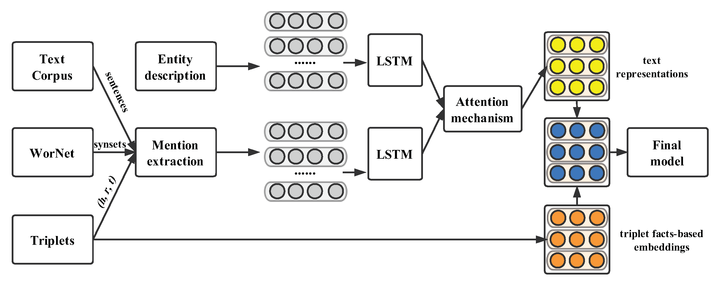
Figure 6 shows a visual process for this model. First, by employing the entity linking tool [86], it can gain the entity text descriptions at the top of the figure. To explore accurate relation-mentioned sentences for a specific fact , the candidates should contain both the marked entities h and t and one or more hyponym/synonym words corresponding to relation r, called mention extraction. Then, the obtained entity text descriptions and mentions are fed into a two-layer bidirectional recurrent neural network (Bi-RNN) to yield high-level text representations. After that, a mutual attention layer [90] that achieves success in various tasks is employed to refine these two representations. Finally, the structure-based representations that previous models generated are associated with the learned textual representations to calculate the embedding vectors.
where denotes the weight factor, , and are the embedding vectors learned from the structural information, , and indicate the distributional representations of textual descriptions, and , , and are the text-enhanced representations forming the final output of this model.
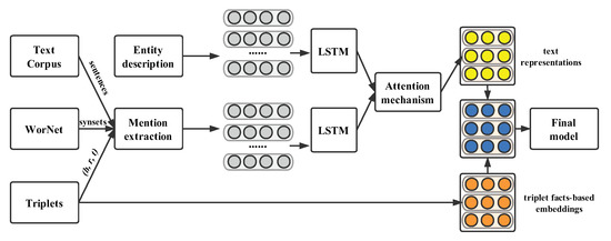
Figure 6.
Framework of text-enhanced KG embedding model.
2.3.2. Relation Path-Based Models
Another category of additional information that can refine the performance of an embedding model is multi-step relational paths, which reveal one or more semantic relations between the entities. Despite that some existing studies, such as TransE, have been a great success in modeling triplet facts, the above approaches only focus on model one-step relation between two entities. Be it different from one-step relation, multi-step relation comprises a sequence of relation paths , and involves more inference information. As an example, the relational path “” demonstrates a relation between and , i.e., .
Lin et al. [30] firstly considered introducing the multi-step relation paths to knowledge graph representation learning. They proposed a path-based embedding model, named PtransE. For each triplet , r denotes the direct relation connecting h and t and is the multi-step relation paths collection between h and t, where is an instance of path. The score function is defined as:
where indicates the normal triplet-based energy score function, which is equal to Equation (3). reflects the authenticity between h and t with multi-step relation paths, and it can be obtained by the below equation:
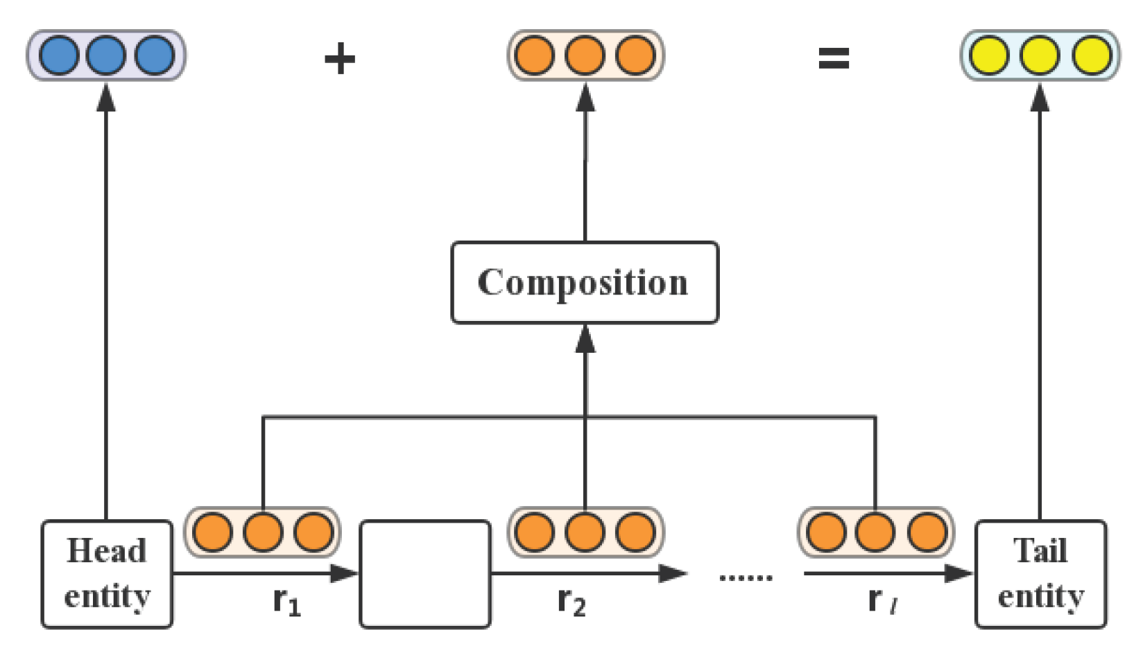
Here, indicates the relation path confidence level of p that is acquired via a network-based resource allocation algorithm [91]. is a normalization factor and signifies the score function for . Therefore, the final problem is how to integrate various relations on the multi-step relation paths p to a uniform embedding vector , as illustrated in Figure 7.
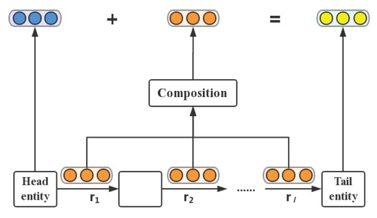
Figure 7.
Framework of the PtransE model.
For this challenge, PtransE applies three representative types of semantic composition operations to incorporate the multiple relation into an embedding vector , including addition (ADD), multiplication (MUL), and recurrent neural network (RNN):
where denotes the embedding vector of relation , represents the combined relation vector at the i-th relation, indicates a composition matrix, signifies the concatenation of , and .
The ADD and MUL versions of PtransE are the extensions of translation-based methods; the RNN version of PtransE and a similar approach proposed by Neelakantan et al. [92] can be considered as the neural network methods’ extension in multiple relation paths. Next, we introduce an extension method based on tensor factorization.
Compared with RESCAL, Guu et al. [93] extended the model by importing multiple relation paths as additional information to enhance the performance. It leverages the multiplication composition to combine different semantic inference information from the relations. The evolved scoring function corresponding to is defined as follows:
where ) are the latent semantic meanings in the relation. The other training processes are the same as previous works and it achieved better performance in answering path queries.
2.3.3. Other Models
Apart from the above methods that use additional information such as textual description and relation paths in Section 2.3, there are also some studies that introduce other information into triplet facts to evolve the traditional methods.
Reference [94,95] suggests that it is necessary to pay attention to the temporal aspects of triplets. For example, happened on 2011; given a date after 2011, it is improper to obtain relations such as where the head entity is . They employ both the observed triplets and the temporal order information of the triplets into the embedding space. Feng et al. [96] proposed a graph-aware knowledge embedding method that considers a KG as a directed graph, applying the structural information of the KG to generate the representations for entities and relations. For more details about graph embedding, please refer to [36].
3. Applications Based on Knowledge Graph Embedding
After introducing the existing knowledge graph embedding methods, we explore diverse tasks and applications that utilize these methods to yield a benefit in this section. These are two types of tasks that are employed to evaluate the performance of embedding models on the most proposed methods, including link prediction and triplet classification. In addition, we introduce the broader domains in which the KG embedding technique can be employed and make contributions, including intelligent question answering systems, recommender systems, and so forth.
3.1. Link Prediction
Link prediction is a common knowledge graph representation application, the goal is to predict a lacking entity when given a concrete entity and relation. More exactly, it intends to predict h when given or r when given , indicated as and . For instance, means to predict who the founder of SpaceX is, and is to inquire about the location of SpaceX.
3.1.1. Benchmark Datasets
Bordes et al. released two datasets for the KG embedding experiment: FB15K [19], which is extracted from Freebase, and WN18 [21], which is generated from WordNet (the datasets are available from https://www.hds.utc.fr/everest/doku.php?id=en:transe). These two datasets are the most extensive benchmarks for this application. Elaborate statistics of these two datasets are shown in Table 5.

Table 5.
The statistics of datasets.
3.1.2. Evaluation Protocol
Given a test triplet , the true tail entity is replaced by every entity e in the entity candidate set. For each iteration, the authenticity of the corrupted triplet is calculated according to the score function . After scoring all triplets in descending order, the rank of is acquired. This whole process is also suitable for the situation with lacking the head entity, i.e., . Further more, two metrics are introduced to evaluate the performance of models: the averaged rank of the correct entities (Mean Rank) and the proportion of the correct entities that ranked in top 10 (HITS@10).
However, not every corrupted triplet is incorrect, some generated triplets also exist in the knowledge graph. In this situation, the rank of the corrupted triplet may be ahead of the original one. To eliminate this problem, all corrupted triplets in which it appears either in the train, validation, or test datasets are filtered out. The raw dataset is named “Raw” and the filtered one is named “Filter”. It is worth to note that the scores with higher HITS@10 and lower Mean Rank denote better performance.
3.1.3. Overall Experimental Results
The detailed results of the link prediction experiment are shown in Table 6. It can be observed that:

Table 6.
Evaluation results on link prediction for different embedding methods.
- Overall, knowledge graph embedding approaches have made impressive progress in the development of these years. For instance, HITS@10(%) in WN18 has improved from the initial 52.8% that RESCAL yielded to 96.4% that R-GCN obtained.
- R-GCN achieves the best performance in the WN18 dataset, but in another dataset, it is not one of the best models. The reason is that R-GCN has to collect all information about neighbors that connect to a specific entity with one or more relations. In WN18, there are only 18 types of relations, it is easy to calculate and generalize. However, FB15K has 1345 types of relations, the computational complexity has increased exponentially for R-GCN, which is why its performance has declined.
- QuatE is superior to all existing methods in FB15K datasets, and is also the second best performing in WN18. It demonstrates that capturing hidden inter-dependency between entities and relations in four-, space is a benefit for knowledge graph representation.
- Compared with the triplet-based models, these description-based models do not yield higher performance in this task. It reveals that external textual information is not fully utilized and exploited; researchers can take advantage of this external information to improve performance in the future.
- In the past two years, the performance of models has not improved much on these two datasets. The most likely reason is that existing methods have already reached the upper bound of performance, so this field needs to introduce new evaluation indicators or benchmark datasets to solve this problem.
3.2. Triplet Classification
Triplet classification is regarded as a binary classification task that focuses on estimating the authenticity of a triplet , proposed by Socher et al. [20].
3.2.1. Benchmark Datasets
Similar to link prediction, this application also has two benchmark datasets, named WN11 and FB13, extracted from WordNet and Freebase (he datasets are available from http://www.socher.org/index.php), respectively. Detailed statistics of the two datasets are shown in Table 5.
3.2.2. Evaluation Protocol
Given a test triplet , a score is calculated via a score function . If this score is above a specific threshold , the corresponding triplet is classified as positive, otherwise as negative. By maximizing the classification accuracy on the validation dataset, we can determine the value of threshold .
3.2.3. Overall Experimental Results
Detailed results of the triplet classification experiment are shown in Table 7. It can be observed that:

Table 7.
Evaluation results on triplets classification accuracy (%) for different embedding methods.
- In summary, these knowledge graph representation learning models have achieved a greater improvement on the WN11 dataset than FB13 because there is twice as much training samples in FB13 as in WN11, but relations between the two datasets are similar in number. This also means that FB13 has more data to train embedding models, thus it improves the generalization ability of models and makes their performance gap smaller.
- In the triplet-based models, TransG outperforms all existing methods in the benchmark datasets. It reveals that multiple semantics for each relation would refine the performance of models.
- Similar to the last task, the description-based models also do not yield impressive improvements in triplet classification application. Especially in recent years, few articles utilize additional textual or path information to improve the performance of models. There is still a good deal of improvement space be achieved with additional information for knowledge graph embedding.
3.3. Other Applications
Apart from the aforementioned applications that are appropriate for KG embeddings, there are other wider fields to which KG representation learning could be applied and play a significant role.
Question answering (QA) systems are a perpetual topic in artificial intelligence, in which the goal is teaching machines to understand questions in the form of natural language and return a precise answer. For the past few years, the QA systems based on KGs have received much attention and some studies have been proposed in this direction [97,98]. The core idea of these methods is to embed both a KG and question into a low-, vector space to make the embedding vector of the question and its corresponding answer as close as possible. This technology also can be used in recommender systems [99,100], which are systems capable of advising users regarding items they want to purchase or hold, and other promising application domains.
However, the applications based on KG embedding are still in their initial stages; in particular, there are few related studies in external applications, such as question answering, and the domains in which researchers are concerned are very limited. Thus, this direction holds great potential for future research.
4. Conclusions and Future Prospects
In this paper, we provide a systematic review of KG representation learning. We introduce the existing models in concise words and describe several tasks that utilize KG embedding. More particularly, we first introduce the embedding models that only apply triplet facts as inputs, and further mention the advanced approaches that leverage additional information to enhance the performance of the original models. After that, we introduce a variety of applications including link prediction and triplet classification, etc. However, the studies on KG embedding are far from mature, and extensive efforts are still required in this field.
To the best of our knowledge, these are three research directions that can be extended: (i) Although those models that utilize the information of additional semantic information are more efficient than the triplet fact-based models, the types of information they can incorporate are extremely limited. The available multivariate information such as hierarchical descriptions between entities/relations in KG, textual Internet information, and even the extracted information from other KGs, can also be applied to refine the representation performance of the embedding models. (ii) The capability of knowledge inference is also a significant part in knowledge graph embedding models. For instance, there is no direct relationship between the head entity and tail entity t in the original KG, but we can explore the inherent connection between these two entities by employing a KG embedding model; this would be greatly beneficial for question answering systems and other applications. Nonetheless, when the relation paths between entities become longer, existing models cannot effectively solve multiple complex relation path problems. Using deep learning technology to integrate all relevant semantic information and represent it uniformly is an alternative solution to this issue. (iii) Although KG representation learning applies to relatively few domains/applications at present, by adopting new technologies such as transfer learning [101], existing models could be applied to a new field with minor adjustments; we believe that this technique will expand to more domains and bring a great improvement compared to traditional methods. We hope that this brief future outlook will provide new ideas and insights for researchers.
Author Contributions
Conceptualization, Y.D. and S.W.; methodology, W.G.; software, Y.D.; validation, Y.D. and S.W.; formal analysis, Y.D., W.G. and N.N.X.; investigation, Y.D.; data curation, Y.D.; writing—original draft preparation, Y.D.; writing—review and editing, W.G. and N.N.X.; supervision, N.N.X.; project administration, S.W., W.G. and N.N.X.; funding acquisition, W.G. All authors have read and agreed to the published version of the manuscript.
Funding
This work is supported by the Guiding Project of Fujian Province under Grant No. 2018H0017.
Conflicts of Interest
The authors declare no conflict of interest.
References
- Pease, A.; Niles, I.; Li, J. The suggested upper merged ontology: A large ontology for the semantic web and its applications. In Proceedings of the Working Notes of the AAAI-2002 Workshop on Ontologies and the Semantic Web, Edmonton, AB, Canada, 28–29 July 2002; Volume 28, pp. 7–10. [Google Scholar]
- Suchanek, F.M.; Kasneci, G.; Weikum, G. Yago: A core of semantic knowledge. In Proceedings of the 16th International Conference on World Wide Web, Banff, AB, Canada, 8–12 May 2007; pp. 697–706. [Google Scholar]
- Bollacker, K.; Evans, C.; Paritosh, P.; Sturge, T.; Taylor, J. Freebase: A collaboratively created graph database for structuring human knowledge. In Proceedings of the 2008 ACM SIGMOD International Conference on Management of Data, Vancouver, BC, Canada, 9–12 June 2008; pp. 1247–1250. [Google Scholar]
- Vrandečić, D.; Krötzsch, M. Wikidata: A free collaborative knowledgebase. Commun. ACM 2014, 57, 78–85. [Google Scholar] [CrossRef]
- Auer, S.; Bizer, C.; Kobilarov, G.; Lehmann, J.; Cyganiak, R.; Ives, Z. Dbpedia: A nucleus for a web of open data. In Proceedings of the Semantic Web, International Semantic Web Conference, Asian Semantic Web Conference, ISWC 2007 + ASWC 2007, Busan, Korea, 11–15 November 2007; pp. 722–735. [Google Scholar]
- Shen, W.; Wang, J.; Luo, P.; Wang, M. Linden: Linking named entities with knowledge base via semantic knowledge. In Proceedings of the 21st International Conference on World Wide Web, Lyon, France, 16–20 April 2012; pp. 449–458. [Google Scholar]
- Shen, W.; Wang, J.; Luo, P.; Wang, M. Linking named entities in tweets with knowledge base via user interest modeling. In Proceedings of the 19th ACM SIGKDD International Conference on Knowledge Discovery and Data Mining, Chicago, IL, USA, 11–14 August 2013; pp. 68–76. [Google Scholar]
- Zheng, Z.; Si, X.; Li, F.; Chang, E.Y.; Zhu, X. Entity disambiguation with freebase. In Proceedings of the 2012 IEEE/WIC/ACM International Joint Conferences on Web Intelligence and Intelligent Agent Technology, Macau, China, 4–7 December 2012; pp. 82–89. [Google Scholar]
- Damljanovic, D.; Bontcheva, K. Named entity disambiguation using linked data. In Proceedings of the 9th Extended Semantic Web Conference, Crete, Greece, 27–31 May 2012; pp. 231–240. [Google Scholar]
- Dong, L.; Wei, F.; Zhou, M.; Xu, K. Question answering over freebase with multi-column convolutional neural networks. In Proceedings of the 53rd Annual Meeting of the Association for Computational Linguistics and the 7th International Joint Conference on Natural Language Processing, Beijing, China, 26–31 July 2015; pp. 260–269. [Google Scholar]
- Xu, K.; Reddy, S.; Feng, Y.; Huang, S.; Zhao, D. Question Answering on Freebase via Relation Extraction and Textual Evidence. In Proceedings of the 54th Annual Meeting of the Association for Computational Linguistics, Berlin, Germany, 7–12 August 2016; pp. 2326–2336. [Google Scholar]
- Hoffmann, R.; Zhang, C.; Ling, X.; Zettlemoyer, L.; Weld, D.S. Knowledge-based weak supervision for information extraction of overlapping relations. In Proceedings of the 49th Annual Meeting of the Association for Computational Linguistics, Portland, OR, USA, 19–24 June 2011; pp. 541–550. [Google Scholar]
- Fei, W.; Daniel, W. Open information extraction using Wikipedia. In Proceedings of the 48th Annual Meeting of the Association for Computational Linguistics, Uppsala, Sweden, 11–16 July 2010; pp. 118–127. [Google Scholar]
- Sang, S.; Yang, Z.; Wang, L.; Liu, X.; Lin, H.; Wang, J. SemaTyP: A knowledge graph based literature mining method for drug discovery. BMC Bioinform. 2018, 19, 193. [Google Scholar] [CrossRef] [PubMed]
- Abdelaziz, I.; Fokoue, A.; Hassanzadeh, O.; Zhang, P.; Sadoghi, M. Large-scale structural and textual similarity-based mining of knowledge graph to predict drug–drug interactions. J. Web Semant. 2017, 44, 104–117. [Google Scholar] [CrossRef]
- Li, F.L.; Qiu, M.; Chen, H.; Wang, X.; Gao, X.; Huang, J.; Ren, J.; Zhao, Z.; Zhao, W.; Wang, L.; et al. Alime assist: An intelligent assistant for creating an innovative e-commerce experience. In Proceedings of the 2017 ACM on Conference on Information and Knowledge Management, Singapore, 6–10 November 2017; pp. 2495–2498. [Google Scholar]
- Xu, D.; Ruan, C.; Korpeoglu, E.; Kumar, S.; Achan, K. Product Knowledge Graph Embedding for E-commerce. In Proceedings of the 13th International Conference on Web Search and Data Mining, Houston, TX, USA, 3–7 February 2020; pp. 672–680. [Google Scholar]
- Xu, Z.; Zhang, H.; Hu, C.; Mei, L.; Xuan, J.; Choo, K.K.R.; Sugumaran, V.; Zhu, Y. Building knowledge base of urban emergency events based on crowdsourcing of social media. Concurr. Comput. Pract. Exp. 2016, 28, 4038–4052. [Google Scholar] [CrossRef]
- Bordes, A.; Usunier, N.; Garcia-Duran, A.; Weston, J.; Yakhnenko, O. Translating embeddings for modeling multi-relational data. Adv. Neural Inf. Process. Syst. 2013, 2, 2787–2795. [Google Scholar]
- Socher, R.; Chen, D.; Manning, C.D.; Ng, A. Reasoning with neural tensor networks for knowledge base completion. Adv. Neural Inf. Process. Syst. 2013, 1, 926–934. [Google Scholar]
- Bordes, A.; Glorot, X.; Weston, J.; Bengio, Y. A semantic matching energy function for learning with multi-relational data. Mach. Learn. 2014, 94, 233–259. [Google Scholar] [CrossRef]
- Ji, G.; He, S.; Xu, L.; Liu, K.; Zhao, J. Knowledge graph embedding via dynamic mapping matrix. In Proceedings of the 53rd Annual Meeting of the Association for Computational Linguistics and the 7th International Joint Conference on Natural Language Processing, Beijing, China, 26–31 July 2015; pp. 687–696. [Google Scholar]
- Jia, Y.; Wang, Y.; Lin, H.; Jin, X.; Cheng, X. Locally Adaptive Translation for Knowledge Graph Embedding. In Proceedings of the 30th AAAI Conference on Artificial Intelligence, Phoenix, AZ, USA, 12–17 February 2016; pp. 992–998. [Google Scholar]
- Ji, G.; Liu, K.; He, S.; Zhao, J. Knowledge Graph Completion with Adaptive Sparse Transfer Matrix. In Proceedings of the 30th AAAI Conference on Artificial Intelligence, Phoenix, AZ, USA, 12–17 February 2016; pp. 985–991. [Google Scholar]
- Dai, Y.; Wang, S.; Chen, X.; Xu, C.; Guo, W. Generative adversarial networks based on Wasserstein distance for knowledge graph embeddings. Knowl.-Based Syst. 2020, 190, 105165. [Google Scholar] [CrossRef]
- Weston, J.; Bordes, A.; Yakhnenko, O.; Usunier, N. Connecting Language and Knowledge Bases with Embedding Models for Relation Extraction. In Proceedings of the 2013 Conference on Empirical Methods in Natural Language Processing, Seattle, WA, USA, 18–21 October 2013; pp. 1366–1371. [Google Scholar]
- Riedel, S.; Yao, L.; McCallum, A.; Marlin, B.M. Relation extraction with matrix factorization and universal schemas. In Proceedings of the 2013 Conference of the North American Chapter of the Association for Computational Linguistics, Atlanta, GA, USA, 9–14 June 2013; pp. 74–84. [Google Scholar]
- Guo, S.; Wang, Q.; Wang, B.; Wang, L.; Guo, L. Semantically Smooth Knowledge Graph Embedding. In Proceedings of the 53rd Annual Meeting of the Association for Computational Linguistics and the 7th International Joint Conference on Natural Language Processing, Beijing, China, 26–31 July 2015; pp. 84–94. [Google Scholar]
- Ouyang, X.; Yang, Y.; He, L.; Chen, Q.; Zhang, J. Representation Learning with Entity Topics for Knowledge Graphs. In Proceedings of the International Conference on Knowledge Science, Engineering and Management, Melbourne, Australia, 19–20 August 2017; pp. 534–542. [Google Scholar]
- Lin, Y.; Liu, Z.; Luan, H.; Sun, M.; Rao, S.; Liu, S. Modeling Relation Paths for Representation Learning of Knowledge Bases. In Proceedings of the 2015 Conference on Empirical Methods in Natural Language Processing, Lisbon, Portugal, 7–21 September 2015; pp. 705–714. [Google Scholar]
- Toutanova, K.; Lin, V.; Yih, W.T.; Poon, H.; Quirk, C. Compositional learning of embeddings for relation paths in knowledge base and text. In Proceedings of the 54th Annual Meeting of the Association for Computational Linguistics, Berlin, Germany, 7–12 August 2016; pp. 1434–1444. [Google Scholar]
- Zhang, M.; Wang, Q.; Xu, W.; Li, W.; Sun, S. Discriminative Path-Based Knowledge Graph Embedding for Precise Link Prediction. In Proceedings of the European Conference on Information Retrieval, Grenoble, France, 25–29 March 2018; pp. 276–288. [Google Scholar]
- Zhong, H.; Zhang, J.; Wang, Z.; Wan, H.; Chen, Z. Aligning Knowledge and Text Embeddings by Entity Descriptions. In Proceedings of the 2015 Conference on Empirical Methods in Natural Language Processing, Lisbon, Portugal, 17–21 September 2015; pp. 267–272. [Google Scholar]
- Xiao, H.; Huang, M.; Meng, L.; Zhu, X. SSP: Semantic Space Projection for Knowledge Graph Embedding with Text Descriptions. In Proceedings of the 31st AAAI Conference on Artificial Intelligence, San Francisco, CA, USA, 4–9 February 2017; pp. 3104–3110. [Google Scholar]
- An, B.; Chen, B.; Han, X.; Sun, L. Accurate Text-Enhanced Knowledge Graph Representation Learning. In Proceedings of the 2018 Conference of the North American Chapter of the Association for Computational Linguistics: Human Language Technologies, New Orleans, LA, USA, 1–6 June 2018; pp. 745–755. [Google Scholar]
- Cai, H.; Zheng, V.W.; Chang, K. A comprehensive survey of graph embedding: Problems, techniques and applications. IEEE Trans. Knowl. Data Eng. 2018, 30, 1616–1637. [Google Scholar] [CrossRef]
- Wang, Q.; Mao, Z.; Wang, B.; Guo, L. Knowledge graph embedding: A survey of approaches and applications. IEEE Trans. Knowl. Data Eng. 2017, 29, 2724–2743. [Google Scholar] [CrossRef]
- Perozzi, B.; Al-Rfou, R.; Skiena, S. Deepwalk: Online learning of social representations. In Proceedings of the 20th ACM SIGKDD International Conference on Knowledge Discovery and Data Mining, New York, NY, USA, 24–27 August 2014; pp. 701–710. [Google Scholar]
- Cao, S.; Lu, W.; Xu, Q. Grarep: Learning graph representations with global structural information. In Proceedings of the 24th ACM International on Conference on Information and Knowledge Management, Melbourne, Australia, 19–23 October 2015; pp. 891–900. [Google Scholar]
- Tang, J.; Qu, M.; Wang, M.; Zhang, M.; Yan, J.; Mei, Q. Line: Large-scale information network embedding. In Proceedings of the 24th International Conference on World Wide Web, Florence, Italy, 18–22 May 2015; pp. 1067–1077. [Google Scholar]
- Wu, F.; Song, J.; Yang, Y.; Li, X.; Zhang, Z.M.; Zhuang, Y. Structured Embedding via Pairwise Relations and Long-Range Interactions in Knowledge Base. In Proceedings of the 29th AAAI Conference on Artificial Intelligence, Austin, TX, USA, 25–30 January 2015; pp. 1663–1670. [Google Scholar]
- Zhao, Y.; Liu, Z.; Sun, M. Representation Learning for Measuring Entity Relatedness with Rich Information. In Proceedings of the 24th International Joint Conference on Artificial Intelligence, Buenos Aires, Argentina, 25–31 July 2015; pp. 1412–1418. [Google Scholar]
- Liu, Z.; Zheng, V.W.; Zhao, Z.; Zhu, F.; Chang, K.C.C.; Wu, M.; Ying, J. Semantic Proximity Search on Heterogeneous Graph by Proximity Embedding. In Proceedings of the 31st AAAI Conference on Artificial Intelligence, San Francisco, CA, USA, 4–9 February 2017; pp. 154–160. [Google Scholar]
- Nikolentzos, G.; Meladianos, P.; Vazirgiannis, M. Matching Node Embeddings for Graph Similarity. In Proceedings of the 31st AAAI Conference on Artificial Intelligence, San Francisco, CA, USA, 4–9 February 2017; pp. 2429–2435. [Google Scholar]
- Guo, S.; Wang, Q.; Wang, B.; Wang, L.; Guo, L. SSE: Semantically smooth embedding for knowledge graphs. IEEE Trans. Knowl. Data Eng. 2017, 29, 884–897. [Google Scholar] [CrossRef]
- Zhang, C.; Zhang, K.; Yuan, Q.; Peng, H.; Zheng, Y.; Hanratty, T.; Wang, S.; Han, J. Regions, periods, activities: Uncovering urban dynamics via cross-modal representation learning. In Proceedings of the 26th International Conference on World Wide Web, Perth, Australia, 3–7 April 2017; pp. 361–370. [Google Scholar]
- Han, Y.; Shen, Y. Partially Supervised Graph Embedding for Positive Unlabelled Feature Selection. In Proceedings of the 25th International Joint Conference on Artificial Intelligence, New York, NY, USA, 9–15 July 2016; pp. 1548–1554. [Google Scholar]
- Defferrard, M.; Bresson, X.; Vandergheynst, P. Convolutional neural networks on graphs with fast localized spectral filtering. In Proceedings of the 30th International Conference on Neural Information Processing Systems, Barcelona, Spain, 5–10 December 2016; pp. 3844–3852. [Google Scholar]
- Mikolov, T.; Sutskever, I.; Chen, K.; Corrado, G.; Dean, J. Distributed Representations of Words and Phrases and their Compositionality. Adv. Neural Inf. Process. Syst. 2013, 26, 3111–3119. [Google Scholar]
- Mikolov, T.; Chen, K.; Corrado, G.; Dean, J. Efficient estimation of word representations in vector space. arXiv 2013, arXiv:1301.3781. [Google Scholar]
- Wang, Z.; Zhang, J.; Feng, J.; Chen, Z. Knowledge graph embedding by translating on hyperplanes. In Proceedings of the 28th AAAI Conference on Artificial Intelligence, Québec City, QC, Canada, 27–31 July 2014; pp. 1112–1119. [Google Scholar]
- Lin, Y.; Liu, Z.; Sun, M.; Liu, Y.; Zhu, X. Learning entity and relation embeddings for knowledge graph completion. In Proceedings of the 29th AAAI Conference on Artificial Intelligence, Austin, TX, USA, 25–30 January 2015; pp. 2181–2187. [Google Scholar]
- Nguyen, D.Q.; Sirts, K.; Qu, L.; Johnson, M. STransE: A novel embedding model of entities and relationships in knowledge bases. In Proceedings of the 14th Annual Conference of the North American Chapter of the Association for Computational Linguistics: Human Language Technologies, Dunhuang, China, 9–14 October 2016; pp. 460–466. [Google Scholar]
- Xiao, H.; Huang, M.; Hao, Y.; Zhu, X. TransA: An adaptive approach for knowledge graph embedding. arXiv 2015, arXiv:1509.05490. [Google Scholar]
- Wang, F.; Sun, J. Survey on distance metric learning and dimensionality reduction in data mining. Data Min. Knowl. Discov. 2015, 29, 534–564. [Google Scholar] [CrossRef]
- He, S.; Liu, K.; Ji, G.; Zhao, J. Learning to represent knowledge graphs with gaussian embedding. In Proceedings of the 24th ACM International on Conference on Information and Knowledge Management, Melbourne, Australia, 19–23 October 2015; pp. 623–632. [Google Scholar]
- Kullback, S. Information Theory and Statistics; Courier Corporation: North Chelmsford, MA, USA, 1997. [Google Scholar]
- Jebara, T.; Kondor, R.; Howard, A. Probability product kernels. J. Mach. Learn. Res. 2004, 5, 819–844. [Google Scholar]
- Xiao, H.; Huang, M.; Zhu, X. TransG: A generative model for knowledge graph embedding. In Proceedings of the 54th Annual Meeting of the Association for Computational Linguistics, Berlin, Germany, 7–12 August 2016; Volume 1, pp. 2316–2325. [Google Scholar]
- Miller, G.A. WordNet: A lexical database for English. Commun. ACM 1995, 38, 39–41. [Google Scholar] [CrossRef]
- Nickel, M.; Tresp, V.; Kriegel, H.P. A three-way model for collective learning on multi-relational data. In Proceedings of the 28th International Conference on International Conference on Machine Learning, Bellevue, WA, USA, 28 June–2 July 2011; pp. 809–816. [Google Scholar]
- García-Durán, A.; Bordes, A.; Usunier, N. Effective blending of two and three-way interactions for modeling multi-relational data. In Proceedings of the Joint European Conference on Machine Learning and Knowledge Discovery in Databases, Nancy, France, 15–19 September 2014; pp. 434–449. [Google Scholar]
- Yang, B.; Yih, S.W.t.; He, X.; Gao, J.; Deng, L. Embedding entities and relations for learning and inference in knowledge bases. In Proceedings of the 2015 International Conference on Learning Representations, San Diego, CA, USA, 7–9 May 2015. [Google Scholar]
- Nickel, M.; Rosasco, L.; Poggio, T. Holographic Embeddings of Knowledge Graphs. In Proceedings of the 30th AAAI Conference on Artificial Intelligence, Phoenix, AZ, USA, 12–17 February 2016; pp. 1955–1961. [Google Scholar]
- Plate, T.A. Holographic reduced representations. IEEE Trans. Neural Netw. 1995, 6, 623–641. [Google Scholar] [CrossRef]
- Brigham, E.O.; Brigham, E.O. The Fast Fourier Transform and Its Applications; Pearson: Upper Saddle River, NJ, USA, 1988; Volume 448. [Google Scholar]
- Trouillon, T.; Welbl, J.; Riedel, S.; Gaussier, É.; Bouchard, G. Complex embeddings for simple link prediction. In Proceedings of the International Conference on Machine Learning, New York, NY, USA, 19–24 June 2016; pp. 2071–2080. [Google Scholar]
- Kazemi, S.M.; Poole, D. SimplE embedding for link prediction in knowledge graphs. In Proceedings of the 32nd International Conference on Neural Information Processing Systems, Montreal, QC, Canada, 3–8 December 2018; pp. 4289–4300. [Google Scholar]
- Sun, Z.; Deng, Z.H.; Nie, J.Y.; Tang, J. RotatE: Knowledge Graph Embedding by Relational Rotation in Complex Space. In Proceedings of the International Conference on Learning Representations, New Orleans, LA, USA, 6–9 May 2019. [Google Scholar]
- Zhang, S.; Tay, Y.; Yao, L.; Liu, Q. Quaternion knowledge graph embeddings. In Proceedings of the 33th International Conference on Neural Information Processing Systems, Vancouver, BC, Canada, 8–14 December 2019; pp. 2731–2741. [Google Scholar]
- LeCun, Y.; Bengio, Y.; Hinton, G. Deep learning. Nature 2015, 521, 436. [Google Scholar] [CrossRef]
- Wang, S.; Guo, W. Robust co-clustering via dual local learning and high-order matrix factorization. Knowl. -Based Syst. 2017, 138, 176–187. [Google Scholar] [CrossRef]
- Wang, S.; Guo, W. Sparse multigraph embedding for multimodal feature representation. IEEE Trans. Multimed. 2017, 19, 1454–1466. [Google Scholar] [CrossRef]
- Ke, X.; Zou, J.; Niu, Y. End-to-end automatic image annotation based on deep cnn and multi-label data augmentation. IEEE Trans. Multimed. 2019, 21, 2093–2106. [Google Scholar] [CrossRef]
- Dong, X.; Gabrilovich, E.; Heitz, G.; Horn, W.; Lao, N.; Murphy, K.; Strohmann, T.; Sun, S.; Zhang, W. Knowledge vault: A web-scale approach to probabilistic knowledge fusion. In Proceedings of the 20th ACM SIGKDD International Conference on Knowledge Discovery and Data Mining, Montreal, QC, Canada, 3–8 December 2014; pp. 601–610. [Google Scholar]
- Schmidhuber, J. Deep learning in neural networks: An overview. Neural Netw. 2015, 61, 85–117. [Google Scholar] [CrossRef]
- Goodfellow, I.; Bengio, Y.; Courville, A.; Bengio, Y. Deep learning. Nature 2015, 521, 436–444. [Google Scholar]
- Liu, Q.; Jiang, H.; Evdokimov, A.; Ling, Z.H.; Zhu, X.; Wei, S.; Hu, Y. Probabilistic reasoning via deep learning: Neural association models. arXiv 2016, arXiv:1603.07704. [Google Scholar]
- Nair, V.; Hinton, G.E. Rectified linear units improve restricted boltzmann machines. In Proceedings of the 27th International Conference on Machine Learning, Haifa, Israel, 21–24 June 2010; pp. 807–814. [Google Scholar]
- Nguyen, D.Q.; Nguyen, T.D.; Nguyen, D.Q.; Phung, D. A Novel Embedding Model for Knowledge Base Completion Based on Convolutional Neural Network. In Proceedings of the 2018 Conference of the North American Chapter of the Association for Computational Linguistics: Human Language Technologies, New Orleans, LA, USA, 1–6 June 2018; Volume 2, pp. 327–333. [Google Scholar]
- Schlichtkrull, M.; Kipf, T.N.; Bloem, P.; Van Den Berg, R.; Titov, I.; Welling, M. Modeling relational data with graph convolutional networks. In Proceedings of the European Semantic Web Conference, Anissaras, Greece, 3–7 June 2018; pp. 593–607. [Google Scholar]
- Cai, L.; Wang, W.Y. KBGAN: Adversarial Learning for Knowledge Graph Embeddings. In Proceedings of the 2018 Conference of the North American Chapter of the Association for Computational Linguistics: Human Language Technologies, New Orleans, LA, USA, 1–6 June 2018; Volume 1, pp. 1470–1480. [Google Scholar]
- Robbins, H.; Monro, S. A stochastic approximation method. Herbert Robbins Sel. Pap. 1985, 22, 102–109. [Google Scholar]
- Kingma, D.P.; Ba, J. Adam: A method for stochastic optimization. arXiv 2014, arXiv:1412.6980. [Google Scholar]
- Xie, R.; Liu, Z.; Sun, M. Representation learning of knowledge graphs with hierarchical types. In Proceedings of the 25th International Joint Conference on Artificial Intelligence, Palo Alto, CA, USA, 9–15 July 2016; pp. 2965–2971. [Google Scholar]
- Wang, Z.; Li, J. Text-enhanced representation learning for knowledge graph. In Proceedings of the 25th International Joint Conference on Artificial Intelligence, Palo Alto, CA, USA, 9–15 July 2016; pp. 1293–1299. [Google Scholar]
- Yosef, M.A.; Hoffart, J.; Bordino, I.; Spaniol, M.; Weikum, G. Aida: An online tool for accurate disambiguation of named entities in text and tables. Proc. VLDB Endow. 2011, 4, 1450–1453. [Google Scholar]
- Krompaß, D.; Baier, S.; Tresp, V. Type-Constrained Representation Learning in Knowledge Graphs. In Proceedings of the 14th International Conference on The Semantic Web-ISWC, Bethlehem, PA, USA, 11–15 October 2015; pp. 640–655. [Google Scholar]
- Xie, R.; Liu, Z.; Jia, J.; Luan, H.; Sun, M. Representation Learning of Knowledge Graphs with Entity Descriptions. In Proceedings of the 30th AAAI Conference on Artificial Intelligence, Phoenix, AZ, USA, 12–17 February 2016; pp. 2659–2665. [Google Scholar]
- Vaswani, A.; Shazeer, N.; Parmar, N.; Uszkoreit, J.; Jones, L.; Gomez, A.N.; Kaiser, Ł.; Polosukhin, I. Attention is all you need. In Proceedings of the 31th International Conference on Neural Information Processing Systems, Long Beach, CA, USA, 4–9 December 2017; pp. 5998–6008. [Google Scholar]
- Zhou, T.; Ren, J.; Medo, M.; Zhang, Y.C. Bipartite network projection and personal recommendation. Phys. Rev. E 2007, 76, 046115. [Google Scholar] [CrossRef]
- Neelakantan, A.; Roth, B.; McCallum, A. Compositional Vector Space Models for Knowledge Base Completion. In Proceedings of the 53rd Annual Meeting of the Association for Computational Linguistics and the 7th International Joint Conference on Natural Language Processing, Beijing, China, 26–31 July 2015; pp. 156–166. [Google Scholar]
- Guu, K.; Miller, J.; Liang, P. Traversing Knowledge Graphs in Vector Space. In Proceedings of the 2015 Conference on Empirical Methods in Natural Language Processing, Beijing, China, 26–31 July 2015; pp. 318–327. [Google Scholar]
- Jiang, T.; Liu, T.; Ge, T.; Sha, L.; Li, S.; Chang, B.; Sui, Z. Encoding temporal information for time-aware link prediction. In Proceedings of the 2016 Conference on Empirical Methods in Natural Language Processing, Austin, TX, USA, 1–5 November 2016; pp. 2350–2354. [Google Scholar]
- Trivedi, R.; Dai, H.; Wang, Y.; Song, L. Know-Evolve: Deep Temporal Reasoning for Dynamic Knowledge Graphs. In Proceedings of the International Conference on Machine Learning, San Francisco, CA, USA, 25–27 October 2017; pp. 3462–3471. [Google Scholar]
- Feng, J.; Huang, M.; Yang, Y.; Zhu, X. GAKE: Graph aware knowledge embedding. In Proceedings of the COLING 2016 the 26th International Conference on Computational Linguistics: Technical Papers, Osaka, Japan, 11–16 December 2016; pp. 641–651. [Google Scholar]
- Bordes, A.; Chopra, S.; Weston, J. Question Answering with Subgraph Embeddings. In Proceedings of the 2014 Conference on Empirical Methods in Natural Language Processing, Doha, Qatar, 25–29 October 2014; pp. 615–620. [Google Scholar]
- Bordes, A.; Weston, J.; Usunier, N. Open question answering with weakly supervised embedding models. In Proceedings of the Joint European Conference on Machine Learning and Knowledge Discovery in Databases, Porto, Portugal, 7–11 September 2014; pp. 165–180. [Google Scholar]
- Zhang, F.; Yuan, N.J.; Lian, D.; Xie, X.; Ma, W.Y. Collaborative knowledge base embedding for recommender systems. In Proceedings of the 22nd ACM SIGKDD International Conference on Knowledge Discovery and Data Mining, San Francisco, CA, USA, 13–17 August 2016; pp. 353–362. [Google Scholar]
- Fu, C.; Zhou, M.; Xuan, Q.; Hu, H.X. Expert recommendation in oss projects based on knowledge embedding. In Proceedings of the 2017 International Workshop on Complex Systems and Networks, Doha, Qatar, 8–10 December 2017; pp. 149–155. [Google Scholar]
- Lu, J.; Behbood, V.; Hao, P.; Zuo, H.; Xue, S.; Zhang, G. Transfer learning using computational intelligence: A survey. Knowl. -Based Syst. 2015, 80, 14–23. [Google Scholar] [CrossRef]
© 2020 by the authors. Licensee MDPI, Basel, Switzerland. This article is an open access article distributed under the terms and conditions of the Creative Commons Attribution (CC BY) license (http://creativecommons.org/licenses/by/4.0/).

