Abstract
In this paper, a novel hardware architecture for neuroevolution is presented, aiming to enable the continuous adaptation of systems working in dynamic environments, by including the training stage intrinsically in the computing edge. It is based on the block-based neural network model, integrated with an evolutionary algorithm that optimizes the weights and the topology of the network simultaneously. Differently to the state-of-the-art, the proposed implementation makes use of advanced dynamic and partial reconfiguration features to reconfigure the network during evolution and, if required, to adapt its size dynamically. This way, the number of logic resources occupied by the network can be adapted by the evolutionary algorithm to the complexity of the problem, the expected quality of the results, or other performance indicators. The proposed architecture, implemented in a Xilinx Zynq-7020 System-on-a-Chip (SoC) FPGA device, reduces the usage of DSPs and BRAMS while introducing a novel synchronization scheme that controls the latency of the circuit. The proposed neuroevolvable architecture has been integrated with the OpenAI toolkit to show how it can efficiently be applied to control problems, with a variable complexity and dynamic behavior. The versatility of the solution is assessed by also targeting classification problems.
1. Introduction
Artificial Neural Networks (ANN) are computational models inspired by the structure and physiology of the human brain, aiming to mimic their natural learning capabilities. ANNs excel in complex tasks, such as computer vision, natural language processing or intelligent autonomous systems, which are difficult to handle by using conventional rule-based programming languages. In addition, biological evolution has inspired the development of evolutionary engineering methods that exploit the benefits of Evolutionary Algorithms (EA) [1] as optimization and solution searching tools. Evolutionary engineering techniques have been applied in areas such as robotics [2], bioengineering [3], electrical engineering [4] or electromagnetism [5]. EAs have also been used to design and adjust digital circuits, which is known as Evolvable Hardware (EH) [6].
Natural learning and biological evolution are not independent processes. Natural brains are themselves products of natural selection. Similarly, EAs can be combined with ANNs to discover computing structures featured with learning capacities. The combination of both bio-inspired fields is known as neuroevolution [7]. It includes techniques to create neural network topologies, weights, building blocks, hyperparameters and even learning algorithms. One of the pioneering algorithms in neuroevolution is NeuroEvolution of Augmenting Topologies (NEAT). NEAT and their variants have been applied to evolve topologies along with weights of small recurrent neural networks, showing outstanding performance in complex reinforcement learning tasks [8,9]. Other researchers have focused on the evolution of deep neural network topologies and the optimizer hyperparameters, substituting handcrafted design and re-design steps with automated methodologies [10]. Deep neuroevolution requires intensive gradient-based training and evolution cycles, only appropriate to cloud facilities.
Differently to the state-of-the-art, a hardware-accelerated integrated solution for neuroevolution is proposed in this paper. In addition to the design automation benefits inherent to neuroevolution and the expected acceleration produced by hardware, implementing a neuroevolvable hardware architecture allows training (and re-training) the neural network, in an edge computing device, during its whole lifetime. This approach enables the continuous adaptation of systems working in dynamic environments. Continuous adaptation is not possible in conventional ANNs that use gradient-based backpropagation algorithms for training since the high computational demands associated with these algorithms require cloud or GPU-based computing resources, not available in the edge. However, the different nature of evolutionary algorithms makes possible the design of custom hardware accelerators for learning weights and topologies to be used directly in the edge.
The proposed neuroevolvable hardware architecture is based on the Block-based Neural Network (BbNN) template, initially conceived in [11]. A BbNN is a particular type of ANN, in which neurons are arranged as a two-dimensional grid of Processing Elements (PEs). Each PE is connected to its four nearest neighbors through four ports (north, south, east and west), which are configurable as inputs or outputs. Internally, each PE features one, two or three artificial neurons, depending on its configuration. The parallelism, regularity and high modularity of the BbNN model make it appropriate to be implemented in hardware. In this paper, we propose using a System-on-a-Chip (SoC) FPGA, in which a dual-core ARM processor and reconfigurable logic are combined in the same chip. The EA is executed in the processor, while candidate BbNN solutions are evaluated in the programmable logic, increasing the evaluation (and inference) throughput.
The size of the BbNN structure determines the complexity of the problems it can solve. It also has a significant impact on training time. The more complex a problem is, the bigger the BbNN has to be. However, bigger networks increase the design space to be explored during evolution, which may even prevent its convergence. Since the optimal size for a given problem is unknown in advance, it may be necessary to discover it by trial and error. In addition, when a network is applied to different problems during different system operation stages, it is expected that its size could be changed. For these reasons, the BbNN implementation we propose in this paper is dynamically scalable. Thus, the BbNN can be scaled up and down in size at run-time during the training process, adapting the number of neurons to the complexity of the task.
Dynamic scalability is achieved by using the Dynamic Partial Reconfiguration (DPR) technique, which allows modifying part of the logic while the rest of the device continues working. The proposal of this paper consists in composing the network at run-time by replicating the primary PE of the network, taking benefit of its regularity. This strategy reduces the memory footprint and the time required for scaling the network. It is enabled by the advanced reconfiguration capabilities provided by the IMPRESS [12,13] reconfiguration tool. Moreover, advanced fine-grain reconfiguration features are used in the proposed architecture to modify the parameters of the network during evolution, without requiring a global configuration infrastructure reaching each PE. Differently, the device reconfiguration port is used to modify the configuration parameters by writing the appropriate positions in the device configuration memory. This approach also reduces configuration time and resource occupancy.
The run-time adaptation features provided by the proposed architecture are applied in this work for controlling Cyber-Physical Systems (CPSs) working under dynamic conditions. Different environments included in the OpenAI toolkit [14] are used to benchmark the performance of the proposed architecture for control applications. The OpenAI toolkit defines control problems with different complexities. In particular, we have selected the inverted pendulum and the mountain car problems, as the test bench. When applied to control problems, the feedback provided by the environment after applying the actions generated by the BbNN is used as a reward, guiding the evolutionary algorithm. This means that evolvable BbNNs can be considered a form of reinforcement learning. We also prove how the proposed network can be applied in classification problems, such as the XOR.
The original contributions of this paper can be summarized as follows:
- A scalable BbNN hardware architecture with reduced usage of DSPs and BRAMs. The proposed architecture supports feedback loops, includes a novel synchronization mechanism and a simplified implementation of the activation function.
- A novel approach for the network adaptation that exploits the advanced dynamic and partial reconfiguration features offered by the IMPRESS tool to obtain dynamic scalability and an efficient parameter and topology configuration during evolution.
- The integration of the proposed architecture, implemented on an SoC FPGA, with the OpenAI toolkit, conforming a hardware-in-the-loop simulation platform. This platform shows the applicability of the proposed neuroevolvable hardware architecture as a reinforcement learning solution for control problems.
The rest of the paper is organized as follows: first, in Section 2, the basic operation principles and previous works on BbNNs are presented. In Section 3, the different approaches existing in the literature to implement dynamically scalable architectures are discussed. Then, Section 4 describes the proposed implementation for the BbNN architecture, while Section 5 provides the evolutionary algorithm used in this work. A description of how dynamic scalability and fine-grain reconfiguration are implemented in the architecture is included in Section 6. Section 7 provides use cases and implementation results, while conclusions and future work are tackled in Section 8.
2. Block-Based Neural Networks
In this section, the main background concepts related to Block-based Neural Networks and the existing implementations in the literature are described.
2.1. Basic Principles
BbNNs are a type of ANN in which neurons are arranged as a two-dimensional array of n × m PEs, as shown in Figure 1. The number of inputs of the architecture corresponds to the number of columns (m) in the matrix. Outputs are obtained from the PEs in the last row, leaving unconnected those that are not needed. Each PE is linked with its four closest neighbors, at the north, south, east and west directions. PEs placed at the last column are connected to those in the first column, forming a cylinder. Each PE has, therefore, four ports, which are configurable as inputs or outputs. Vertical links can be configured upwards or downwards, and horizontal links can be configured to the right or the left. Depending on the configuration of the ports, different types of processing elements are defined. Thus, PEs with 1-, 2- or 3-inputs (i.e., 3-, 2- or 1-outputs) are possible, up to a total amount of fourteen PE types, as shown in Figure 2. These types result from combining all the PE inputs with the outputs, with the only limitation that every input must be connected to, at least, one output. PEs with all inputs or all outputs are discarded to avoid inconsistencies within the network. Each processing element applies a neuron operator in each port configured as an output. Neuron operators in BbNNs do not differ from traditional units used in ANNs [11]. They perform a weighted addition of all the inputs and transmit the result to the output node, after invoking an activation function [15]. The activation function is non-linear, being the sigmoid or the hyperbolic tangent the most widely used. These functions are applied to introduce non-linear relations in the network, needed to approximate functions that involve non-linear relations between variables. Performing non-linear operations on hardware platforms, such as FPGAs, entails a high logic resource utilization, especially in terms of DSPs or LUTs.
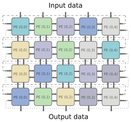
Figure 1.
Block-based Neural Network layout.
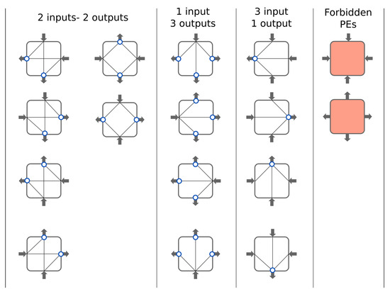
Figure 2.
Processing Element (PE) schemes considered for the Block-based Neural Network.
Since the evolutionary algorithm can decide the direction of every link during the training stage, internal loops may appear. Internal loops feature the network with memory capabilities, so data from a previous state are combined with new data flowing through the network in subsequent time instants. Some examples of feedback loops are shown in Figure 3. Feedbacks are essential when solving time-dependent problems such as control or time series prediction. However, inner loops create data-paths with different lengths, and so they complicate discovering when input data have been completely processed. Knowing when the output data is valid requires synchronizing neuron activities. As it is exposed in Section 4, a synchronization mechanism based on tokens has been implemented in this work.
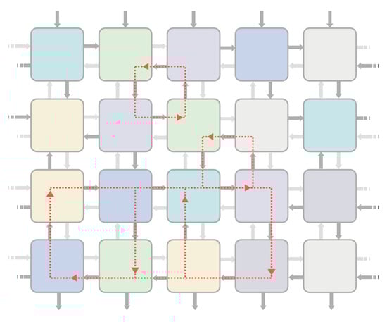
Figure 3.
Inner feedback loops of a Block-based Neural Network (BbNN) configuration.
Authors in [11] demonstrate mathematically that for structures with a maximum of five inputs, the number of interconnections in a BbNN is higher than the corresponding value in a fully connected network. Therefore, BbNNs can replace traditional neural networks with a similar number of inputs while providing parallelism and scalability. Parallelism given by hardware acceleration enhances the throughput of the system, while the high regularity of the BbNN layout facilitates its scalability.
2.2. Related Works
Moon and Kong conceived the BbNN model in 2001 [11], as an alternative to general neural network models, specially designed to be implemented in reconfigurable hardware devices. Beyond the architecture, they also proposed the use of genetic algorithms for optimizing the structure and weights of the network. Following this initial work, various researchers have improved the architecture, the optimization method and the applications of the BbNNs, as described next.
The works by Merchant et al. present significant contributions in terms of the BbNN architectures [16,17]. They implemented a BbNN on an SoC FPGA device, that can be evolved online. In particular, the authors selected a Xilinx Virtex-IIPro FPGA featured with two on-chip PowerPC 405 processors. The EA, which is in charge of adapting the system when the operational environment changes, is executed in the on-chip processor, while the configurable BbNN model runs in the programmable logic. This approach is known as intrinsic evolution, since the EA directly changes the final hardware, instead of evolving it offline, using a software model. In this implementation, the Smart Block-based Neuron (SBbN) is proposed as the basic element of the BbNN. The SBbN is a software-configurable neuron, in which the on-chip processor controls the operation of the neuron. The authors present this approach as an alternative to include all the possible configurations of the neuron simultaneously and then selecting the appropriate one with a multiplexer. Differently, in this work, we propose a dynamically reconfigurable processing element, in which the modification of its functionality is carried out by writing in the device configuration memory. A mechanism for latency control using tokens, inspired by Petri networks, is also proposed in the works by Merchant. The token synchronization of this work is slightly different since our proposal also implements accept signals to avoid overwriting unconsumed data. In contrast to the solution proposed by Merchant, our architecture is fully pipelined, and it allows inner loops. These loops require a proper initialization of the tokens to avoid deadlocks in the network, which is shown in Section 4.4.
A new variant of the BbNN model, known as the Extended Block-based Neuron Network (EBbN), is presented in [18]. In contrast with classic BbNN implementations, the EBbN presents six input/output ports instead of four. However, possible configurations are limited since the north and south ports are always configured downwards. The two east and the two west ports can be configured to provide both side horizontal data flow, right or left data flow, or they may not provide either side data flow. The EBbN has a lower hardware overhead when compared with the SBbN. Authors achieve this by using the internal resources more efficiently since resource redundancy within the PE is eliminated. Pipeline registers are introduced to separate every row in the network. However, the EBbN model cannot be applied on large networks since the critical path still becomes longer as the number of stages increases. Differently, our approach is fully pipelined at all the outputs of each neuron (i.e., at horizontal and vertical directions). This pipeline scheme achieves higher operating frequencies than previous works, and hence the throughput of the proposed architecture is incremented.
Focusing on the implementation of the activation function, some works [16,19,20] present a LUT-based approximation of its non-linear section, where discrete values of the function are stored. This method achieves high accuracy but increases memory utilization unless all the PEs share a single LUT-based function, which in turn, constitutes a bottleneck. An alternative to the LUT-based activation function was presented in [21]. In that work, a sigmoid-like activation function is implemented as a piecewise-quadratic (PWQ) function (i.e., as a function defined by multiple sub-functions).
There have also been contributions in terms of the training algorithms. Although most of the BbNN-based systems are trained by using EAs, some works rely on alternative optimization methods. In [22], the problem is posed as a set of linear equations solved with the linear least-squares method. This approach provides good training accuracy for time-series prediction and nonlinear system identification problems. Authors in [23] propose the use of a multi-population parallel genetic algorithm (GA) targeting implementations on multi-threading CPUs.
Most of the implementations reported for the BbNN do not allow the inner feedback loops defined in the original model. Only in works by Nambiar [21,23] and Kong [11,24], topologies with feedback loops are addressed, showing how these feedback loops can lead to non deterministic results if all the PE outputs are not registered. The authors tackled this issue by introducing latency as a parameter to be controlled by the EA, encoded in the chromosome. In the present work, the uncertainties induced by feedback loops are controlled with the token synchronization.
In previous works, the BbNN model has succeeded in solving tasks of different domains such as classification, time series forecasting and control. In [25], it has been applied to ECG signal analysis and classification, such as arrhythmia detection [26] or driver drowsiness detection [27]. Hypoglycemia detection has been another use case of the BbNN related to the healthcare domain [28]. Time series prediction [22,24] and dynamic parameter forecasting [23] show the BbNN capabilities to solve tasks with temporal dependencies. This ability to solve problems where time is an intrinsic factor makes BbNN a good option to deal with control problems, like mobile control problems [11] or dynamic fuzzy control [29]. Real-time intrusion detection systems have also been developed in [30].
Apart from the works related to BbNNs, there are almost no hardware implementations of neuroevolvable systems providing continuous learning in the state-of-the-art. One of the most relevant works in this regard is the GenSys [31], an SoC prototype that includes an accelerator for the NEAT algorithm and an inference engine that accelerates in hardware the neural networks described by the evolutionary algorithm. At this regard, the work by A.Upegui on the evolution of spiking neural networks using DPR on commercial FPGAs is also notable [32].
In a more general sense, different circuit topologies have been proposed in the state-of-the-art to be used as part of evolvable hardware systems. Relevant examples are the Cartesian Genetic Programming (CGP) [33] or Systolic Arrays (SA) [34]. Both of them are based on meshes of interconnected processing elements that perform different functions from their inputs. In its standard form, the CGP corresponds to a computing graph that is directed and feed-forward. Therefore, a PE may only receive inputs from either input data or the output of a PE in a previous column [33,35]. Connectivity is CGP is achieved by adding large multiplexers at the input of each PE, which has a resource overhead that limits the size of the structure. In turn, SAs do not have such a high connectivity overhead since their dataflow is fixed and restricted to the closest neighbors of each PE.
3. Existing Approaches to Scalability
Scalable architectures offer significant advantages compared to fixed architectures. Their size can be adapted to change the quality of the results, to operate with inputs of different width or to modify its computation performance (e.g., adding more modules to exploit data parallelism). An architecture can be scaled at design-time (e.g., using generics in HDL descriptions [36]), or it can be scaled dynamically to deal with changing external conditions. Dynamic scalability requires using SRAM-based FPGAs, with dynamic partial reconfiguration (DPR) capabilities. DPR makes it possible to adapt part of the device fabric at run-time, while the rest of the system (i.e., the static part) remains uninterrupted. There are two concepts that are important to understand in dynamically reconfigurable systems, which are reconfigurable regions (RRs) and reconfigurable modules (RMs). The RMs are accelerators that can be exchanged in the system at run-time. On the other hand, the RRs are regions of the FPGA that have been reserved for allocating the RMs. This section introduces different approaches found in the literature to implement dynamically scalable architectures.
The most direct way to implement scalable architectures is to synthesize offline different variants of the same accelerator, with different sizes, and then to swap them in one Reconfigurable Region (RR) of the FPGA. This approach has been used in [37] to generate a scalable family of two-dimensional DCT (discrete cosine transform) hardware modules aiming at meeting time-varying constraints for motion JPEG. A similar approach is used in [38] to vary the deblocking filter size to adapt it to different constraints in H.264/AVC coding. In [39], the authors implement a CORDIC accelerator that can be scaled at run-time to work with different data types when the required dynamic range and accuracy change. A sharp drawback of this approach is that the whole RR remains occupied when the size of the architecture decreases, so it can not be reused for other modules.
A more efficient alternative to achieve real footprint scalability is to create several RRs, as shown in Figure 4a, and changing the size of the architecture by replicating modules in parallel. With this approach, free RRs can be reused for other RMs. This approach has been used in [40] with four RRs to allocate a scalable H.264/AVC deblocking filter. When the architecture can not be divided into different RMs, it is possible to arrange contiguous RRs in slot or grid styles [41]. In these configurations, one RM can be allocated in several RRs, as shown in Figure 4b. In this way, when the size of the architecture increases, the RM can use more RRs. This approach has been used in [42] to generate an architecture for DCT computation with three size levels that can be allocated in up to three contiguous slots.
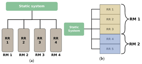
Figure 4.
(a) Scalable architecture using multiple isolated reconfigurable regions connected to the static system. (b) Scalable architecture using multiple reconfigurable regions arranged in a slot style, where one reconfigurable module (RM) can span multiple reconfigurable regions (RRs).
The previous approaches can be used when the modules are connected directly to the static system. However, they are not valid in two-dimensional mesh-type architectures (e.g., BbNNs or systolic arrays) that have direct interconnections among neighboring processing elements. The most natural solution to interconnect RMs is to use static resources crossing the boundaries of their RRs. This approach is followed in [43], where the authors generate a triangular systolic array architecture for computing the DCT. The systolic array can be scaled using different RRs that can allocate a whole diagonal of PEs. The main drawback of this approach is that the communication among RRs is fixed, and therefore, it is not very easy to reuse the RRs for other accelerators. The authors in [44] solve this problem by using switching boxes that can be configured to adapt the interconnection among the PEs.
Using static but configurable interconnections among PEs offers excellent flexibility at the cost of having a considerable resource overhead. It is possible to reduce this overhead by using reconfigurable interfaces instead of a fixed infrastructure. A reconfigurable interface is composed of specific device routing nodes located at the border of the PE; if a neighbor module uses a compatible set of nodes in its interface, the communication between neighboring modules is enabled without requiring fixed interconnections. The authors in [34,45] used this approach to build a scalable systolic array for evolvable hardware and a scalable wavefront array to implement a deblocking filter. In both cases, the static system contains one RR that interfaces with the static system through specific nodes located at the border of the RR. The RR does not have static resources, and therefore it can be deemed as a grid-based RR that can allocate multiple PEs. In this way, the same RR can allocate several architectures with different communication schemes. Authors relied on the academic tool Dreams [46] to build these applications since commercial tools did not, and still do not provide these advanced reconfiguration features.
It must be noticed that every module of the architecture does not have a fixed position in the device when its size changes. This fact limits the connection of the scalable architecture with the static system. The solution provided by the authors is to use only one input/output module located in one corner of the RR and to surround the architecture with communication and control modules that communicate the outer blocks of the architecture with the input/output instance. When using this approach, the RR can allocate several modules. One example could be connecting the static system to the 4 corners of the RR and allocating two-dimensional architectures or monolithic reconfigurable modules, as shown in Figure 5. In this case, the architectures can only grow at the expense of reducing the size of the other modules.
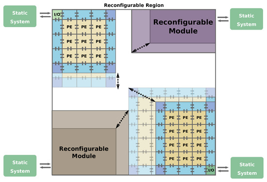
Figure 5.
Scalable architectures using reconfigurable interconnections.
4. Proposed Bbnn Architecture
This section describes the reconfigurable and scalable architecture proposed to implement BbNNs in hardware. It aims to reduce the utilization of resources while keeping modularity and scalability. First, we focus the discussion on the implementation of the processing elements used as the basic building block for the BbNN. Then, the modules used for connecting the neurons and handling data within the network are described.
Each PE in the BbNN computes a variable number of outputs (K) with a given number of inputs (J) using the following expression:
where:
- g: is the activation function of the neuron.
- : is the input of the neuron.
- : is the is the connection weight between the input and the output.
- : is the bias applied to the output.
- : is the output of the neuron.
These arithmetic operations are proposed in the original model to be computed as floating-point numbers, including the non-linear activation function. A set of numerical optimizations are proposed first to provide an optimized hardware implementation.
4.1. Numerical Optimizations
We have studied first the most convenient fixed-point data representation and the approximation of the activation function to be used in the proposed hardware implementation.
4.1.1. Numerical Range for Inputs and Parameters
The numerical range has a straightforward impact on the hardware resource utilization and the size of the chromosomes used during training since the algorithm directly evolves these values. Therefore, it also affects the size of the design space to be explored.
In this work, we have decided to use a range of (−4, 4). Experimentally, we have validated that this range is appropriate to activate or deactivate the network nodes during training. This choice is also coherent with the proposals existing in the literature. For instance, in [21], authors use the range of [−3, +3]. Notice that in both cases, the number of bits required for the representation of the integer part is the same. The complete fixed-point representation scheme is explained in the next section.
4.1.2. Fixed-Point Representation Scheme
A fixed-point representation has been chosen for the input data and all the intermediate computations, aiming at reducing the logic resources required when compared to the floating-point counterpart. We now describe the details of the selected representation, which is graphically shown in Figure 6.
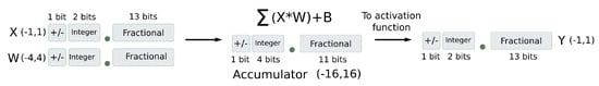
Figure 6.
Fixed-point representation used in this work.
All the registers and data ports are implemented using 16 bits. Since the integer part requires three bits to allocate the integer range of (−4, 4), 13 bits remain for the fractional part. This scheme is used for inputs, weights and bias, but it is modified for the internal neuronal computations within a PE. The maximum number of concurrent connections to a single PE output is 3, as shown in Figure 2. It corresponds to a PE with a single output and three inputs, represented by Equation (2). Considering that weights have been limited to the range (−4, 4), the range of values passed to the activation function is (−16, 16) as Equation (3) illustrates. The integer part of these values can be represented with 4 bits, plus an extra bit for the sign.
Instead of enlarging the accumulation registers inside the PE, we opt for redistributing the 16 bits as follows. We dedicate now the 5 bits required for the integer part and the remaining 11 bits for the fractional part. This decision reduces the flip-flops required for the implementation of each PE.Output data from the activation function and input data to the PE are coded with the same fixed-point representation. Figure 6 shows the data representation at each computation stage.
4.1.3. Approximation of the Activation Function
We use the sigmoid function as the activation function since it has proven in the literature to provide good results when used in BbNNs [21,25]. Other well-known activation functions reported in the neural network literature, such as the Rectified Linear Unit (ReLU), could also be appropriate from the algorithmic point of view. However, we have discarded the functions that are not constrained to a value range, which creates overflows and inconsistencies when dealing with fixed-point data types in hardware implementations.
As mentioned in Section 2, some authors used an LUT-based approximation for the approximation of the non-linear function, where discrete values of the sigmoid function are stored in pre-computed look-up tables. Thus, computing the activation function is reduced to finding in the table the value corresponding to the required point. However, this look-up table constitutes a bottleneck if multiple PEs require simultaneous access to this table. In an architecture with massive parallelism like BbNNs, sharing the activation function has a considerable impact on the processing throughput. As an alternative, piecewise quadratic (PWQ) functions can approximate the sigmoid without the necessity of LUTs. PWQ function technique implies performing multiplications, which require the usage of DSP units.
Differently, the proposal of this work consists in splitting the function domain into sub-functions whose operands can be represented as the addition of powers of 2, as shown in Equation (4). The selection of the appropriate sub-function (i.e., the corresponding tranche of the function) is carried out by evaluating the integer part () of the function argument. In turn, the fractional part () is used to compute the output within each sub-function, by applying bit-shifting transformations.
In Figure 7, the comparison of the approximate sigmoid function and the real function is exposed. Mean squared error between both functions in the non-linear section is . This error is only calculated for the (−6, 6) range since out of this range the sigmoid function is practically linear.
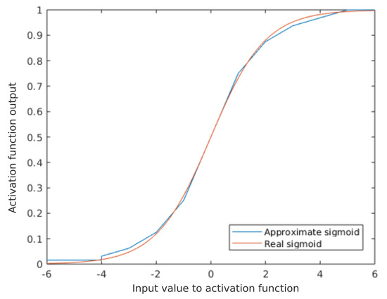
Figure 7.
Comparation of the approximate sigmoid function and the real function.
4.2. Proposed Processing Element Architecture
As shown in Figure 8a, the interface of the processing element includes the following signals:
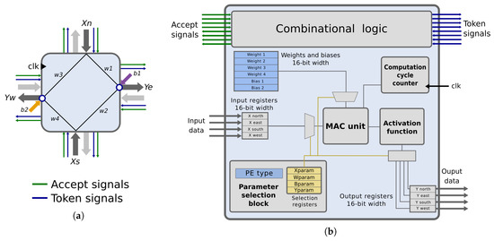
Figure 8.
Proposed structure for the BbNN processing element. (a) Shows the interface and internal connections of one possible type of processing element (PE). (b) Exposes internal blocks of a generic PE.
- Input data: one input signal per PE side (, , , )
- Output data: one output signal per PE side (y, y, y, y).
- Token signals: one token signal per input/output port. They are part of the synchronization mechanism. They indicate that intermediate results are ready to be consumed. They are set to one by the producer PE and set to zero by the consumer PE.
- Accept signals: one accept signal per input/output port. These signals avoid overwriting unconsumed data. They are also part of the token-based synchronization scheme. Accept signals are set to zero when the consumer has not consumed inputs or while it is triggered, and they are set to one when the link has no data, and the consumer PE is idle.
Each PE is characterized by a set of parameters, represented as blue boxes in Figure 8b. These parameters fully define the behavior of the PE, including the PE type, the weights and the biases. They are implemented with LUTs that can be configured using the fine-grain reconfiguration technique detailed in Section 6. This way, each PE of the BbNN is configured without the need for a global configuration infrastructure. Thus, enhancing the scalability of the BbNN.
Apart from the PE parameters, each PE is composed of the following modules:
- Parameter selection block: it generates the signals that select the proper operands at the right clock cycles depending on the values stored in the parameter selection registers (Xparam, Wparam, Bparam and Yparam). These values are chosen from the PE type.
- MAC Unit: it performs all the calculations to generate the weighted sum during the computation cycle.
- Computation cycle counter: this counter controls the computation cycle stage.
- Activation function: this block computes the approximation of the sigmoid function, as it was described in the previous section.
- Synchronization logic: this logic checks the values of the token signals to trigger the computation cycle. When the operations are executed, it generates the output ports tokens. This logic also manages the accept signals.
Only one DSP per PE is needed, which is included in the MAC Unit. All the calculations of the neuron block are performed throughout seven clock cycles. The DSP is used sequentially during these clock cycles performing multiply and accumulate (MAC) operations with the appropriate operands. During the computation cycle, the Parameter Selection Block generates selection signals to indicate which input, weight, bias value and output is required at each cycle. This selection depends on the coded sequence stored in the fine-grain reconfigurable LUTs of the Parameter Selection Block. These values constitute the internal configuration of the PE. Once the weighted sum of a neuron’s output is ready, its value is passed to the activation function block to generate the final output value. Table 1 illustrates how each parameter of the neuron is encoded.

Table 1.
Signal coding for parameter selection.
The operations carried out in the seven clock-cycles are shown with an example in Figure 9. In the first clock cycle, the triggering condition of the PE is checked, and the values stored in the accumulator from previous clock cycles are reset. If the triggering condition is fulfilled, the PE parameters are read sequentially and decoded on the subsequent clock cycles. This decoding uses the values in Table 1 to generate the selection signals for each operand and the proper output at each clock cycle. Each neuron type has an unique codification for each selection signal (SelX, SelY, SelB and SelY).

Figure 9.
Values of the selection parameter register for the subscribed neuron type and read sequence.
Not all PE types require the seven clock cycles to compute the output. This value is defined by the worst case, which corresponds to a PE with the maximum number of outputs (i.e., 1-input/3-outputs). As the DSP is used sequentially, the accumulated results must be reset before computing a different PE output. With three outputs, two clock cycles are needed per output: one clock cycle to multiply the input and the corresponding weight, and an extra clock cycle to reset the accumulator. Therefore, six clock cycles are used as computation cycles, besides the additional clock cycle needed to check the triggering condition. In any case, the clock cycles not required by a given PE are lost, since all the PEs are synchronized every seven clock cycles.
4.3. From the Basic PE to the Block-Based Neural Network IP
The proposed BbNN has been integrated into an Intellectual Property (IP) core, as shown in Figure 10. The main component of the IP is the BbNN itself. At design-time, the BbNN is a dummy block reserved in a reconfigurable region. This reconfigurable region is then used to allocate PEs at run-time to compose a BbNN of a given size. The composition of the BbNN is carried out by reconfiguring individual PEs into the reconfigurable region. Each PE has compatible interfaces to neighboring PEs so that they connect directly without predefined static interconnections. Composing the BbNN in this modular way allows scaling its size efficiently by adding or removing PEs.
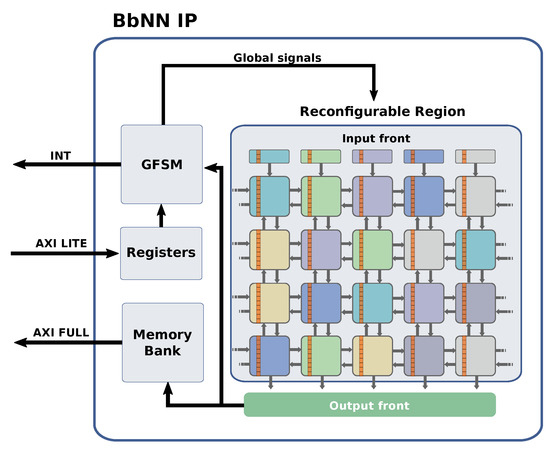
Figure 10.
Block-based Neural Network Intellectual Property (IP) with fine-grain reconfigurable elements in each PE.
Once the BbNN has been composed, it can be configured using a technique called fine-grain reconfiguration that has been used in state of the art to reconfigure specific elements of an FPGA (e.g., LUTs) [47,48]. In the proposed BbNN each PE parameter (e.g., weights, biases) is implemented using LUTs whose output values can be modified by adapting the LUTs truth table using fine-grain reconfiguration. The IP also contains specific logic to provide the inputs to the BbNN via fine-grain reconfiguration. This way, a direct connection between the BbNN and the static system is not required, which enhances the scalability of the network. However, output signals are connected through the southern border of the reconfigurable region, independently of the size of the network. A memory bank accessible by the processor using an AXI interface has been included to store the outputs temporarily.
In summary, the proposed BbNN implementation relies on dynamic partial reconfiguration to (1) compose the BbNN on the fly by stitching together individual neuron blocks, (2) change the configuration of each neuron in the training phase and (3) providing the input values to the network. Details regarding the scalability and the configuration of the BbNN are described in Section 6.
The processor is also connected to the BbNN IP through an AXI lite interface that can be used to modify the BbNN configuration registers. These registers can be used to enable or disable the BbNN, asserting that a new input has been provided to the network or to select which network outputs are used. The General Finite State Machine (GSFM) controller is the component that reads the registers written by the user and writes the necessary control signals to the BbNN. These signals are connected to every PE of the network. To allow scalability, these signals use specific routing resources of the FPGA reserved to clocks and other global signals. Once the BbNN generates a set of valid outputs, the GSFM asserts an interrupt signal to indicate that the processor can read the output values and generate a new input signal.
4.4. Management of Latency and Datapath Imbalance
All the PE outputs include a pipeline register to keep the critical path of the circuit constant regardless of the BbNN configuration. Therefore, the latency of the network depends on the length of the paths between the inputs and outputs. By latency, we mean the number of cycles needed to process all the BbNN inputs until a valid output is generated. Since the dataflow is fully configurable, this latency is variable. This circumstance is shown in Figure 11, where two BbNN configurations with the same size and selected output, but different dataflows, are represented. Configuration in Figure 11a has a latency of 10 cycles, and configuration Figure 11b has a latency value of 18 cycles.
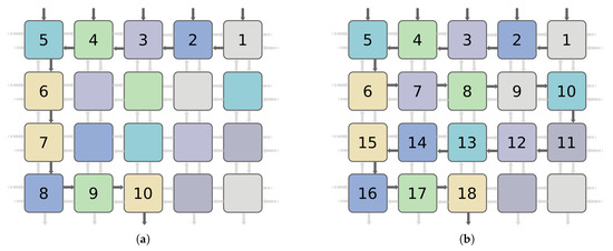
Figure 11.
Configurations with the same dimensions and selected output but different latency. (a) shows a configuration with a 10 latency cycles; meanwhile (b) exposes a configuration with 18 latency cycles.
The dependency of the datapath length with the network configuration might also cause the computing imbalance at the PE level. If two paths arriving the same PE have different lengths, valid data will arrive at the PE at different control steps. In this work, the network latency and the datapath imbalance are controlled with a synchronization scheme based on tokens and accept signals. When an output from a neuron is ready to be used, a token is set at the pertinent link. PEs are only triggered if all the tokens at their input nodes are activated. Accept signals avoid overwriting a link with unconsumed data. This approach may cause deadlocks during the first calculation cycle if the BbNN configuration under test has feedback loops. Neurons influenced by feedback loop wait for other neurons in the loop to produce an output, leading to a deadlock. This scenario is avoided by setting to one the tokens in the upward vertical links by default at the first calculation cycle.
5. Proposed Evolutionary Algorithm
This section presents the EA used as the optimization mechanism in the proposed BbNN. EAs have been selected for driving the training of the network since they require fewer memory resources and a lower numerical precision when compared with other alternatives, including gradient-based methods. This makes them suitable for their intrinsic implementation in the SoC. The EA runs on the processor of the system, and its goal is to optimize data structures called chromosomes. These chromosomes encode complete configurations of the network, including weights, biases and port directions for every PE. BbNN codification within the chromosome structure is exposed in Figure 12. The size of the chromosome depends on the BbNN size. Larger networks require larger chromosomes since the EA uses a direct encoding. Weights and biases of each PE are represented with 16-bits per parameter (see Figure 12a). Dataflow configuration of the whole network is encoded with two bitstrings: E_param for East ports and N_param for North ports. Two bits per PE are needed to configure the dataflow. Figure 12b shows an example of the dataflow configuration generated by this combination of parameters. Therefore, each PE adds 98 bits to the chromosome size. A problem-dependent fitness score is assigned to every chromosome during the evaluation stage. This value is stored in each chromosome with a float variable. Each chromosome also has an associated age, whose functionality is explained next in this section, stored as an integer variable.
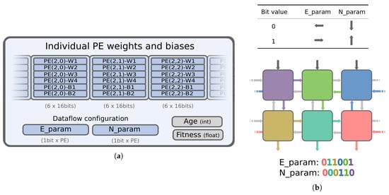
Figure 12.
BbNN configuration encoded in the chromosome structure. (a) presents the representation of the chromosome structure. (b) exposes and example of dataflow configuration from bits in E_param and N_param.
The proposed algorithm is detailed in Algorithm 1. The algorithm takes as many iterations (generations) as needed to achieve a fitness score that exceeds the value defined as the target. The initial population of chromosomes is created randomly (line 1). At every generation, a mutation operator is applied over the whole population of chromosomes with different mutation rates (line 6). Thus, producing copies of the chromosomes with altered data. These copies are the offspring. The portion of altered data injected by the mutation operator is given by the mutation rate, which in the proposed algorithm decays in chromosomes with high fitness values. Therefore, good chromosomes suffer lighter mutations. Decaying the mutation rate enhances the performance of the algorithm since aggressive mutations on the dataflow may worsen the behavior of chromosomes with a high fitness value. In turn, chromosomes with undesired performance are removed from the population with two mechanisms: extinction and age threshold.
Each chromosome has an associated age. This value is incremented if any offspring chromosome improves the performance of the original one (line 12). A chromosome is removed if its age is over the maximum age, defined as an algorithm parameter (lines 13–15). This mechanism prevents the stalling of the evolutionary algorithm. After some generations, the extinction operator is applied over chromosomes with the lowest fitness values (lines 19–22). This strategy constitutes a kind of elitism: only the best chromosome is protected from extinction. Extinction is the second mechanism to prevent the algorithm from stalling while it increases the diversity of the population, thus avoiding to fall into local minimum points. All operators of the proposed EA are configurable with the parameters represented in Table 2. The values of these parameters have been set empirically to enhance the convergence of the EA. Another mechanism to prevent the stalling of the EA is the dynamic scalability of the network. If fitness value remains constant for several generations, the EA scales up the architecture by adding a row to the network.
Table 2.
Parameters of the Evolutionary Algorithm.
The design of the fitness function is crucial for accomplishing a successful evolution process. This function must be adapted to the problem by the designer. In classification problems, the goal of the function is to assign a high score to chromosomes that result in higher classification accuracy. Meanwhile, in control problems, the fitness function is designed to assign high scores to those chromosomes which behavior achieves the requirements for the physical problem to be considered as solved. The design of each fitness function for each of the use cases described in this work is detailed in Section 7.
| Algorithm 1: Evolutionary algorithm |
 |
6. A New Approach to Build a Scalable Bbnn
Enhancing the BbNN model with dynamic scalability allows handling the size of the network as a parameter to be optimized at run-time, instead of being fixed at design-time. This way, the optimization algorithm can find the appropriate size, as a trade-off between the size of the design space under exploration and the capability of the architecture to undertake complex problems. Dynamic scalability is also useful in applications in which changing the network size leads to different quality levels. In these applications, it is possible to adapt the size of the BbNN according to different run-time constraints, such as energy consumption, quality of results or available logic resources in the FPGA.
Its modular design and the distributed nature of its control make the BbNN an excellent candidate to be implemented in a grid-based RR, using specific reconfigurable interfaces. The proposed implementation is possible thanks to the use of the advanced reconfiguration features provided by the IMPRESS reconfiguration tool [12,13]. IMPRESS is an open-source (https://des-cei.github.io/tools/impress) design tool developed by the authors targeting the implementation of reconfigurable systems. IMPRESS has been designed with a particular focus on implementing scalable two-dimensional mesh architectures (i.e., overlays). Some features of IMPRESS that are of significant importance to build scalable overlays are the following: direct reconfigurable-to-reconfigurable interfaces, module (i.e., bitstream) relocation, the implementation of multiple RMs in the same clock region and decoupling the implementation of the static system and the reconfigurable modules. All these features allow the reconfiguration of multiple individual PEs in a single RR to compose at run-time a BbNN of any given size. Another feature of IMPRESS that is of great importance to implement scalable BbNNs is the possibility to instantiate LUT-based constants inside reconfigurable modules. This feature, known as fine-grain reconfiguration, allows changing these logic constants by reconfiguring a single device frame that spans one clock region column. A frame is the minimum reconfigurable unit of an FPGA. Fine-grain reconfiguration accelerates the reconfiguration of logic constants distributed throughout the device fabric. LUT-based reconfigurable components can be used to access the inside of a RR without needing a direct link to the static system. In the case of BbNNs, the purpose of fine-grain reconfiguration is twofold. First, it allows changing the configuration of the PEs without using any global bus interface. It also enhances scalability as it is possible to provide inputs to the network without using external communication modules that add overhead to the system.
The following is a description of the process of building a scalable BbNN with the aid of IMPRESS. First, it is necessary to generate the static system with a single RR that contains the interface of the output BbNN blocks. The interface of the RR can be easily defined by selecting which border (e.g., south) is used, and then IMPRESS automatically selects which routing nodes are used as interface points. Figure 13a shows an example of an empty RR with a south interface. The next step is implementing the reconfigurable PE. IMPRESS allows relocating reconfigurable modules in different RRs, whenever they have the same resource footprint (i.e., regions with the same resource distribution). Once all the modules have been implemented, it is possible to compose a BbNN of arbitrary size at run-time by reconfiguring individual blocks, as shown in Figure 13b. Notice that contrary to the Xilinx reconfiguration flow where each RM has to be allocated in a unique RR, IMPRESS can allocate inside a single RR multiple RMs that are interconnected to each other through reconfigurable interfaces.
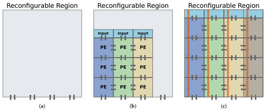
Figure 13.
(a) Empty reconfigurable region. (b) reconfigurable region with 3 × 3 BbNN. (c) reconfigurable region with 4 × 4 BbNN showing LUT-based constants grouped in columns.
During the run-time training of the BbNN, it is necessary to configure each PE of the BbNN to modify the weights, biases and the neuron type configuration. Fine-grain reconfiguration needs to be fast enough to be usable in the training phase of the BbNN, where a large number of potential candidate configurations have to be evaluated. To reduce the reconfiguration time, IMPRESS automatically groups all the LUT-based constants in the same column of device resources so that all the constants can be reconfigured by modifying a minimum amount of frames. This feature makes fine-grain reconfiguration fast enough to be used in the training phase of the BbNN. Fine-grain reconfiguration can also be used to enhance scalability. As explained before, the works presented in [34,45] surrounded the scalable architectures with communication and control modules that passed the input/output signals to the corresponding modules. This strategy can lead to considerable resource overhead for small overlays. This overhead is avoided in this work by providing the inputs to the BbNN with fine-grain reconfiguration. Figure 13c shows an example of a scalable BbNN with fine-grain constants grouped in columns to modify the BbNN configuration and the input modules.
As we have seen, the BbNN relies on two different reconfigurations techniques. The first one is used to allocate RMs inside the RR to change the size of the BbNN. The BbNN size is usually selected before launching the application. However, the EA can change it at run-time if the fitness value is stalled after a given number of generations, as shown in the experimental results. The second technique is the fine-grain reconfiguration, which is used to provide the inputs of the BbNN and also to configure the BbNN parameters during the training phase.
One difficulty that arises when building scalable BbNNs with reconfigurable interfaces and fine-grain reconfiguration is how to connect the edges of the network. This means, to close the structure as a cylinder, which is a convenient feature to increase the connectivity between input variables. The proposed implementation connects the edges by routing the signals through the interior of the BbNN, as shown in Figure 14. This approach increases the heterogeneity of the PEs. Instead of using the same RM, this solution requires three different RMs depending on the location (i.e., center or edge of the BbNN), which hinders PE relocation. Moreover, bypass signals crossing the BbNN form a combinatorial path which size increases with the size of the BbNN. When building larger BbNNs, these routes can become the critical path, thus limiting the maximum system frequency. In the cases where the maximum frequency limit is achieved, it is possible to connect dummy blocks (i.e., blocks that output a constant value) at the edges of the BbNN. While this solution does not connect the edges of the BbNN, it has the advantage that it keeps the frequency of the system independent of the BbNN size.
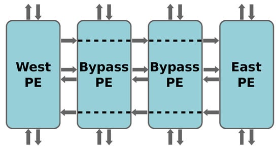
Figure 14.
Connecting the external edges of the BbNN using reconfigurable interconnections.
Figure 15a shows the implementation of the BbNN static system in a Xilinx Zynq xc7z020clg400-1 SoC, including the area reserved for the RR. The RR can be populated at run-time with PEs to compose a BbNN with up to 3 × 5 neurons. Figure 15b shows the implementation of the different neurons and input modules and how they can be arranged at run-time to compose a 1 × 5 BbNN. It is important to remark that the BbNN is rotated compared to the one shown in Figure 15c. In this case, the data flow goes from the west to the east. This modification allows placing all the input modules in the same column, aligning all the fine-grain reconfigurable inputs in the same frame. Thus, speeding-up the reconfiguration process. The main drawback of rotating the BbNN is that it hinders the relocation of the neurons in the column. PEs in the bottom and top columns have a different interface to those in the middle of the column, and therefore their partial bitstreams are not compatible with relocation.
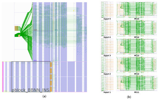
Figure 15.
(a) Shows a BbNN static system implementation that can allocate up to 3 × 5 PEs. (b) Shows how neuron blocks can be arranged inside the reconfigurable region at run-time to form a 1 × 5 BbNN.
IMPRESS incorporates a library to manage the reconfiguration of mesh-type architectures. This library includes a bidimensional variable that represents the current configuration of the architecture. Each element in this variable has two parameters. The first one is a pointer to a reconfigurable module in the library. The second one is the location where the reconfigurable module is allocated in the device. When any of these parameters are changed, IMPRESS automatically initiates the reconfiguration process to allocate the specified reconfigurable module in the desired FPGA location.
Moreover, IMPRESS includes a run-time hardware reconfiguration engine specialized for fine-grain reconfiguration. The reconfiguration engine receives the configuration of the constants, and it automatically reconfigures the FPGA with the required configuration.
7. Results
This section illustrates the performance of the system in terms of logic resource utilization, the reconfiguration time and the capability to resolve different problems in two different domains, which are classification and control tasks.
7.1. Logic Resource Utilization and Reconfiguration Times
Table 3 contains the resource utilization of the static system and each PE in the BbNN implementation shown in Figure 15. The static system includes the BbNN controller, the fine-grain reconfiguration engine and an empty RR where the BbNN PE blocks can be allocated at run-time. Table 3 also shows the resources used by each individual processing element. Each PE uses 473 LUTS, 163 flip-flops and 1 DSP. As the PE can be implemented in different reconfigurable regions, there are small variations in the percentage of used resources among RRs. The size of the partial bitstreams also depends on the region where the PE is implemented. The PE bitstream size varies from 21.8 kB to 26.9 kB, depending on the reconfigurable region where the PE is implemented, while the input module bitstream size is 5.8 kB.
Table 3.
Resource utilization of the BbNN implemented on a Zynq XC7Z020.
As shown in Figure 14, the PE can adopt three different configurations, which have to be implemented as three different RMs. To implement each possible BbNN size, we have to analyze all the possible locations where the RMs can be allocated. The bypass RMs can only be allocated in the inner regions of the RR. However, the edge RMs (e.g., west and east PEs) can be placed in every region except the opposite edge regions (i.e., a west RM cannot be allocated on the east side of the RR). When using the Xilinx reconfiguration flow, it is necessary to generate one partial bitstream for each RM location, which would result in 33 (12 × 2 for edge RMs and 9 for the bypass RM) different partial bitstreams to generate all possible combinations. However, generating all the possible combinations is avoided by the flexibility benefits provided by IMPRESS, which allows relocating one partial bitstream to compatible regions (i.e., regions that have the same resource distribution). In the BbNN implementation shown in Figure 15, the total number of partial bitstreams needed to generate all the possible combinations is reduced to 9.
Table 4 shows a comparison of the proposed PE implementation and existing proposals in the state-of-the-art in terms of logic resources. The proposed architecture presents the lowest footprint in memory elements and DSPs. This is achieved by the proposed implementation for the sigmoid function and the strategy proposed to reuse the single DSP over different clock cycles. The downside of the dynamic scalability and flexibility of the proposed architecture is reflected in the high utilization of logic elements. This logic overhead is a consequence of the online training feature. One downside of dynamic partial reconfiguration is that other circuits cannot use the unused resources of the reconfigurable region where the PE is implemented. Table 3 shows that in our PE proposal, the LUTs are the bottleneck and leave several FFs, DSP and BRAMs unused.
Table 4.
Resource utilization per individual PE in comparison with other works in the state-of-the-art.
Table 5 shows the breakdown of the time spent in each operation stage, both during the training and the inference phases. The time the BbNN needs to process a set of inputs depends on the latency. In a 3 × 3 BbNN, the maximum latency is 9. As each PE needs 7 clock cycles to compute its outputs, the BbNN takes a maximum of 63 clock cycles to make the computation, which results in 0.63 s at 100 MHz. The transference of inputs to the BbNN is carried out using the fine-grain reconfiguration engine, and it takes 6.1 s. In turn, the outputs are read with the AXI interface in 4.3 s. Therefore, the maximum throughput in the inference phase is 90.66 Kilo Operations per second (KOPS). By operation, we mean to process a new set of inputs completely to obtain the desired output from the BbNN. In the training phase, it is also necessary to configure the BbNN. The configuration of each parameter of the BbNN also relies on the fine-grain reconfiguration, and it takes 41.7 s. In the training phase, it is also necessary to take into account the time required by the software to calculate the fitness and to generate the chromosomes, which is application dependant. The computing times for fitness computation are reported next for each use case. All the design operates at 100 MHz, except the fine-grain reconfiguration engine that works at 175 MHz. While the ICAP configuration port has a nominal value of 100 MHz, it has been demonstrated in [50] that it is possible to overclock it at higher frequencies without behavior malfunction. This overclocking aims at reducing the total time needed to reconfigure the BbNN during evolution.
Table 5.
Time breakdown for a 3 × 3 BbNN.
Table 6 shows how the BbNN size impacts the time spent in each stage. Reconfiguration times shown in the table are a consequence of how IMPRESS carries out the fine-grain reconfiguration process, which is described next. First, when the evolutionary algorithm commands to change one parameter in an RM, IMPRESS has to search the device column where the parameter is placed and then modify the column configuration accordingly. Once the user has changed all the parameters, the new configuration values are sent to the reconfiguration engine, a hardware component in charge of reconfiguring the selected columns with the new configuration data. The time spent on this first stage depends on the number of parameters that have to be changed. In contrast, the second phase only depends on the number of columns that have to be reconfigured. In the implementation shown in Figure 15a, the number of frames that have to be reconfigured increases with the BbNN depth. Therefore, the BbNN configuration time of a 3 × 3 BbNN increases significantly compared to a 1 × 3 BbNN. However, when increasing the width of the BbNN, the number of frames that have to be reconfigured is kept constant, thus resulting in a more efficient reconfiguration process. Table 6 shows that increasing the size from a 3 × 3 to a 3 × 5 BbNN results in a more efficient reconfiguration time, especially in the case of the input data that only increases 0.5 s. The increment in the BbNN configuration time is higher because more parameters have to be changed in the first phase of the reconfiguration process.
Table 6.
Performance comparison for different BbNN sizes.
Table 6 also shows the comparison between using fine-grain reconfiguration (working at 175 MHz) and using an AXI lite interface in a non-reconfigurable BbNN operating at 100 MHz. Using fine-grain reconfiguration to configure the BbNN parameters is more efficient than using an AXI lite interface for all the three different sizes. In contrast, the best option to transfer the input data to the BbNN depends on the number of inputs. Fine-grain reconfiguration is convenient when there are five inputs, while the AXI lite interface is the preferred option when the BbNN only contains three inputs.
7.2. Case Studies
This section provides three different case studies showing how the neuroevolvable hardware system can be adapted to different problems. All the results provided are the average of 100 training processes. The EA finishes if a candidate configuration achieves the goal fitness or 1000 generations are exceeded. At each generation, 150 candidate configurations (i.e., chromosomes) are evaluated.
We expose here one classification problem and two control problems. In the classification problem, each chromosome is evaluated with all samples in the dictionary. In control problems, a new set of initial states is evaluated at each generation to avoid inconsistent solutions.
7.2.1. Classification Domain: The Xor Problem
The XOR problem involves two inputs and one output, all 1-bit width. The goal is to evolve the BbNN, so it behaves like a logic XOR gate. If two inputs have the same value, the output is zero. Otherwise, the output must be one.
This problem is solved by using the truth table of the XOR gate as the reference. The selected output of the BbNN is compared with the reference result for each input data pair. The fitness function used to evaluate each configuration is based on the mean squared error of the BbNN output and the reference (see Equation (5)). Both values are float data type. The fitness function expresses the accuracy of the chromosome to approximate the output values to the binary values of the XOR truth table. A fitness over 0.9 corresponds to a mean squared error below 10% for the four cases in the XOR truth table. This problem is considered solved if the achieved fitness is over 0.9.
Fitness computation for this problem takes 21 s, and it is executed once per sample in the batch. The batch contains four samples, so the fitness is computed four times per chromosome. Figure 16 shows the fitness progression along the evolution process and Figure 17 the selected configuration for a 2 × 2 network that solves the problem. It should be noted that the links connecting the edges of the network are used by the solution (i.e., the structure is closed as a cylinder). Figure 18 and Table 7 show the influence of the BbNN size in training. Experimental results showed that the minimum BbNN that can solve this task is a 2 × 2 BbNN. BbNNs with more than 2 × 2 elements facilitate the evolution towards a solution evaluating fewer configurations.
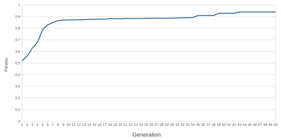
Figure 16.
Progression of the fitness value during the XOR training for a 2 × 2 BbNN.
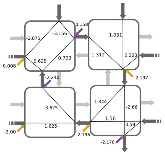
Figure 17.
Solution for the XOR problem.
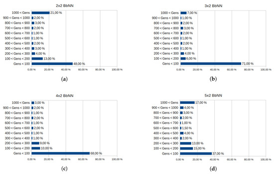
Figure 18.
Influence of the BbNN size in the convergence of the algorithm for XOR problem. Each graph exposes the data from 100 executions of the EA. The generations needed to achieve a solution are segmented in intervals, from 0 to 1000 generations. Executions over 1000 generations are stopped. Convergence of different BbNN sizes is analyzed: 2 × 2 BbNN (a), 3 × 2 BbNN (b), 4 × 2 BbNN (c) and 5 × 2 BbNN (d).
Table 7.
Influence of the BbNN size on the training process for the XOR problem. Average stats from 100 convergent training processes.
The four graphs in Figure 18 show the influence of the BbNN size on the convergence of the XOR problem. For each size, the generations needed by the EA to solve the problem are registered. Each graph covers up to 1000 generations. Beyond this value, the execution of the EA is considered as non-convergent. From these measurements, it can be concluded that the more convenient BbNN size for XOR proves to be 4 × 2 BbNN since it has the lowest rate of non-convergent executions and the highest rates of executions below 100 generations. This BbNN size has the lowest number of evaluated chromosomes and generations on average, as exposed in Table 7.
If the complexity of the classification problem is unknown at run-time, the dynamic scalability of the BbNN may take an essential role in the search for solutions. This situation is shown for the XOR problem in Figure 19. The system starts by searching for a solution with a 1 × 2 BbNN structure. After a period with the fitness stalled completely, the system dynamically adds a new row of PEs to the BbNN (at generation 211, in Figure 19). After a few iterations with the new size, the neuroevolutionary system is able to find a solution. The EA does not support population where chromosomes encode BbNN of different sizes, but it can recompose a new BbNN architecture and reset the evolution process if the fitness does not show any improvement.
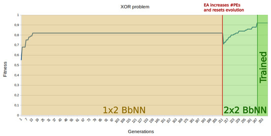
Figure 19.
Resolution of the XOR problem using the dynamic scalability feature. At generation 211 the Evolutionary Algorithm (EA) increases the BbNN size and resets evolution. At generation 249 the EA converges towards a solution.
7.2.2. Control Domain: Mountain Car
The Mountain Car is a standard control problem. It involves a car whose starting position is at the bottom of a valley. The car must reach the top of the hill at the right. The engine of the car is not powerful enough to reach the goal position by accelerating up the slope. Therefore, the car needs to gain momentum to reach it by oscillating from left to right.
A simulation environment for the Mountain Car problem is included in the Gym OpenAI [14] toolkit (Figure 20). The observation space of the environment has two variables: the position of the car and the speed. Both variables are float type that are transformed to the fixed-point representation before being processed by the network. Three possible actions can be performed on the car: push left, push right or do not push. The force of the engine is constant.
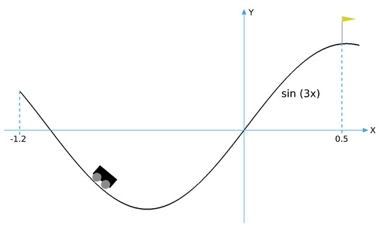
Figure 20.
OpenAI Mountain Car environment and coordinate system used to determine the position of the car. The hills are generated with the sin(3x) function.
The BbNN is evolved to find a controller for this problem directly by interacting with the environment. The Zynq-7020 SoC FPGA device in which the neuroevolvable hardware system runs has been integrated as a hardware-in-the-loop platform with the OpenAI simulator running on a PC. The evaluation of each candidate circuit is called an episode. Each episode finishes when the car reaches the goal position, or after 200 control actions (steps). This value has been obtained experimentally after observing that beyond this number of actions, the likelihood that an unsuccessful candidate circuit reaches the final position decreases.
A specific fitness function has been developed for this environment, which is shown in Equation (6). This fitness function rewards circuits able to drive the car close to the desired position with the fewest possible number of steps. Position of the car is its X coordinate according to Figure 20. It can vary in the range (−1.2, 0.5), the fitness expression presents three possible scenarios:
- Fitness score in the range (−0.12, 0): the steps component in the fitness function is equal to zero since the circuit performs 200 control actions without any success. The car is far from the goal position at the end of the episode.
- Fitness score in the range (0, 0.05): the steps component is also null because all control actions were consumed, but the circuit can drive up the car near the desired position.
- Fitness score over 0.05: circuits scored in this range can drive the car to the goal position in less than 200 steps. The fewer control actions needed, the higher the score is. We consider that achieving the top of the hill with 150 steps can be considered good behavior. This corresponds to a fitness score over 0.4, which is set as the threshold to consider a problem as solved.
Fitness computation for this problem takes 41 s. Fitness is computed once at the end of each episode and hence once per chromosome. An example of the evolution of fitness in an episode is shown in Figure 21.
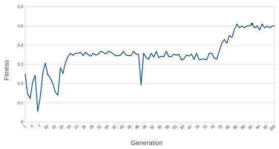
Figure 21.
Example of progression of the fitness value during the Mountain Car training for 2 × 2 BbNN.
Table 8 exposes the influence of the BbNN size on the training process. We only consider topologies with two columns since this is the number of observable variables in the environment. The number of rows varies from 2 to 4. First, we can see that all the considered BbNNs can solve the problem, even with a single row. However, the size has a direct effect on the performance of the EA. Small network architectures need fewer generations to solve the problem since chromosomes have fewer parameters to be optimized. A 1 × 2 BbNN needs 323 generations on average to converge to a solution; meanwhile, 2 × 2 BbNN increases the number of generations needed. Although networks over 1 × 2 size need more generations to be optimized, they enhance the quality of the solution. A 2 × 2 BbNN achieves a good compromise between the best fitness and evaluated circuits.
Table 8.
Influence of the BbNN size on the training process for Mountain Car problem. Average stats from 100 training processes.
Figure 22 provides the convergence of the EA for different BbNN sizes similar to the previous problem. In this case, the smallest BbNN architecture ensures the convergence of the 81% executions below 100 generations and has a low rate of non-convergent executions. Moreover, this BbNN size presents the lowest average generations in Table 8. Therefore, 1 × 2 BbNN is the most suitable size in this case.
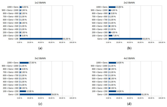
Figure 22.
Influence of the BbNN size in the convergence of the algorithm for Mountain Car problem. Each graph exposes the data from 100 executions of the EA. The generations needed to achieve a solution are segmented in intervals, from 0 to 1000 generations. Executions over 1000 generations are stopped. Convergence of different BbNN sizes is analyzed: 1 × 2 BbNN (a), 2 × 2 BbNN (b), 3 × 2 BbNN (c) and 4 × 2 BbNN (d).
7.2.3. Control Domain: Cart Pole
Cart Pole or Inverted pendulum is a staple problem in the control domain. The center of mass of the pendulum is above its pivot point. Therefore, the pendulum is unstable if no control actions are performed on it. OpenAI also provides a python-based simulation environment for this problem, whose graphical representation is shown in Figure 23.

Figure 23.
Cart Pole environment.
Four variables are observed in the environment: the position and speed of the cart, the angle of the pole and the speed at the end of the pole. All of them are float type variables with different ranges. The system must keep the pole in a balanced position. Two actions can be performed on the simulation environment: push the cart left or right.
In this case, an episode finishes if the angle of the pole is over 12 or the position of the cart exceeds the scenario boundaries. In those cases, the pole is considered to be unbalanced. After each control action on the pole, a partial error value is calculated. This value represents the instability of the pole after the control action. The partial error involves the four parameters of the observation space and their maximum value, as shown in Equation (7). If the pole falls, global fitness is calculated as the addition of all partial error. Not performed steps are scored with the highest partial error value, as shown in Equation (8):
where:
- : is the parameter in the observation space.
- : is the maximum value in the range of parameter in the observation space.
- : represents the instability of the pole after the control action.
Fitness function showed in Equation (8) is designed to assign high scores to those chromosomes that complete 200 control actions in balance and low partial error. Fitness computation for this problem takes 46 s. Fitness is computed after each control action since it involves an accumulation of the partial error. The ultimate fitness would be 1 in case the pole last for 200 control actions in a balanced and static position. However, two chromosomes able to balance the pole during 200 control actions can have different fitness scores since every partial error value depends on the value of the four variables of the observation space. The problem is solved if a fitness value over 0.95 is achieved. An example of the progression of fitness during a Cart Pole training experiment for 3 × 4 BbNN is shown in Figure 24.
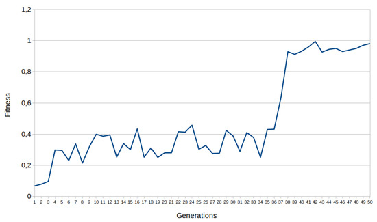
Figure 24.
Example of progression of the fitness value during the Cart Pole training for 3 × 4 BbNN.
The minimum BbNN width for this problem is four: one column for each variable in the observation space. The minimum network size compatible with this control problem is, therefore, 1 × 4 BbNN. Networks with an additional row to 2 × 4 BbNN broaden the design space exploration, and the EA evaluates more configurations to encounter a solution. Additional rows on the architecture have the same effect. Table 9 and graphs in Figure 25 exposes the influence of the BbNN size on the training process. These data have been gathered similarly to former case studies. In this case, increasing the size of the network leads to higher rates of non-convergent executions. Therefore, the most suitable size for this problem is 1 × 4 BbNN, which has the lowest rate of non-convergent executions (Figure 25) and the lowest average generations needed to solve the problem (Table 9).
Table 9.
Influence of the BbNN size on the training process for Cart Pole problem. Average stats from 100 training processes.
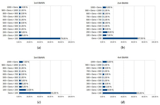
Figure 25.
Influence of the BbNN size in the convergence of the algorithm for Cart Pole problem. Each graph exposes the data from 100 executions of the EA. The generations needed to achieve a solution are segmented in intervals, from 0 to 1000 generations. Executions over 1000 generations are stopped. Convergence of different BbNN sizes is analyzed: 1 × 4 BbNN (a), 2 × 4 BbNN (b), 3 × 4 BbNN (c) and 4 × 4 BbNN (d).
Figure 24 contains the fitness progression of 3 × 4 BbNN during the training process of the Cart Pole problem. The initial unbalanced condition of the pole is different from each generation. Therefore, the same BbNN configuration varies its fitness value depending on the initial state. Figure 26 presents a solution to this problem in which the evolutionary algorithm has created two feedback loops.
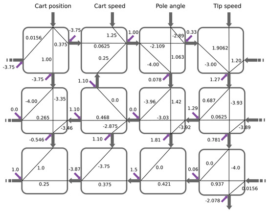
Figure 26.
BbNN solution for Cart Pole problem.
7.3. Online Adaptation for Control in Dynamic Environments
As proof of the online adaptation capability of the proposed system, two examples based on the previous control problems are provided. Both online training examples are tackled following the same approach. First, the system is trained under normal conditions, and once it is capable of controlling the problem for at least 10 generations, physical parameters are changed. This change hampers the capability of the trained BbNN to solve the initial problem. Table 10 exhibits the initial conditions for each problem and their modified values.
Table 10.
Initial and modified conditions for online training.
Some of these modifications to the problem conditions emulate changing the environment. For instance, the modified value of the engine power of the car in the Mountain Car problem emulates a loss of power in the engine. Other changes emulate conditions that harden the problem resolution. For instance, an increment of the gravity over the pole seems unrealistic but creates a handicap for the problem resolution.
Both control problems exhibit similar behavior. After the change in the conditions, a drop in the fitness can be observed. The re-training stage has better average fitness than the first training stage. This means that the system has prior knowledge about the problem, creating a nice basis to solve it when harder conditions appear. Figure 27 and Figure 28 show the evolution of the fitness when conditions change for both control problems.
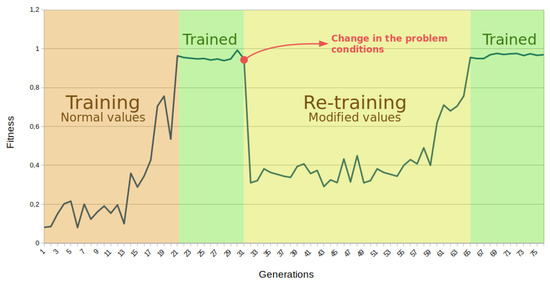
Figure 27.
Cart Pole training and re-train for 3 × 4 BbNN.
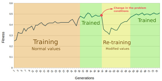
Figure 28.
Mountain Car training and re-train for 2 × 2 BbNN.
8. Conclusions and Future Work
In this paper, we propose a dynamically scalable hardware implementation of the Block-based Neural Network model, which, under the control of an evolutionary algorithm, enables continuous system adaptation. The proposed neuroevolvable hardware system integrates advanced reconfiguration features that allow to (1) compose the BbNN at run-time by stitching together individual PEs and (2) providing the inputs and changing each PE configuration with reduced reconfiguration times. The result is a scalable BbNN whose size can be adapted to the computational demands required by a given application. Experimental results show how scalability allows changing the number of logic resources occupied by the network depending on the complexity of the problem or the expected quality of the results. The proposed system has been implemented in an SoC FPGA and integrated using a hardware-in-the-loop scheme with the OpenAI toolkit to show its efficiency in reinforcement learning problems, such as the cart pole and the mountain car problem.
Regarding resource utilization, each PE uses 473 LUTs, 163 FFs and 1 DSP. Compared to other state-of-the-art solutions, our proposal uses more LUTs but reduces the number of FFs or DSPs. Fine-grain reconfiguration has been proven to be a valid solution to train the BbNN online as all the parameters of a 3 × 3 BbNN can be reconfigured in just 41.7 s. In real applications, it is not necessary to change all the parameters at the same time, which further reduces the total time needed to configure the network. The inputs of the network are also provided using fine-grain reconfiguration in 6.1 s while the outputs are transferred using an AXI full interface in 4.3 s. The time needed to compute the fitness is application-dependent and ranges from 21 s to 46 s for the use cases provided in this paper.
Further research will be carried out to extend the reinforcement learning capabilities of the proposed solution in more complex scenarios and other applications. Different variants of the evolutionary algorithm will also be explored to increase the capacity of the system to deal with more complex problems. Moreover, the evolutionary algorithm will be modified to use the size of the BbNN as an additional parameter subject to evolution, which will allow selecting the most appropriate BbNN size for a given application without user intervention. The fixed-point data encoding of the network can be an obstacle when solving complex problems. Therefore, more precise encoding schemes, like dynamic fixed-point or wider bit width of registers, will be studied. This improvement in data representation may cause an increment in FPGA resource consumption. Other optimization algorithms, such as gradient descend based or multi-threaded EAs will be analyzed, as an alternative to EAs.
Author Contributions
A.G. has contributed to the conceptualization, methodology, investigation, validation, writing—original draft preparation and writing—review and editing. R.Z. has contributed to the conceptualization, methodology, investigation, validation and writing—original draft preparation. A.O. has contributed to the conceptualization, methodology, investigation and writing—original draft preparation. E.d.l.T. has contributed to the investigation and writing—original draft preparation. All authors have read and agreed to the published version of the manuscript.
Funding
This research was partially funded by the European Union’s Horizon 2020 research and innovation programme under grant agreement No 732105 (CERBERO Project).
Conflicts of Interest
The authors declare no conflict of interest. The funding sponsors had no role in the design of the study; in the collection, analyses, or interpretation of data; in the writing of the manuscript, and in the decision to publish the results.
References
- Goldberg, D.E. Genetic Algorithms in Search, Optimization and Machine Learning, 1st ed.; Addison-Wesley Longman Publishing Co., Inc.: Boston, MA, USA, 1989. [Google Scholar]
- Alattas, R.J.; Patel, S.; Sobh, T.M. Evolutionary modular robotics: Survey and analysis. J. Intell. Robot. Syst. 2019, 95, 815–828. [Google Scholar] [CrossRef]
- Kriegman, S.; Blackiston, D.; Levin, M.; Bongard, J. A scalable pipeline for designing reconfigurable organisms. Proc. Natl. Acad. Sci. USA 2020, 117, 1853–1859. [Google Scholar] [CrossRef] [PubMed]
- Zebulum, R.S.; Pacheco, M.A.; Vellasco, M. Comparison of different evolutionary methodologies applied to electronic filter design. In Proceedings of the 1998 IEEE International Conference on Evolutionary Computation Proceedings, IEEE World Congress on Computational Intelligence (Cat. No. 98TH8360), Anchorage, AK, USA, 4–9 May 1998; pp. 434–439. [Google Scholar]
- Hornby, G.; Globus, A.; Linden, D.; Lohn, J. Automated antenna design with evolutionary algorithms. In Space 2006; American Institute of Aeronautics and Astronautics: Reston, VA, USA, 2006; p. 7242. [Google Scholar]
- Sekanina, L. Virtual Reconfigurable Circuits for Real-World Applications of Evolvable Hardware. In Proceedings of the 5th International Conference on Evolvable Systems: From Biology to Hardware, Wuhan, China, 21–23 September 2007; pp. 186–197. [Google Scholar] [CrossRef]
- Stanley, K.O.; Clune, J.; Lehman, J.; Miikkulainen, R. Designing neural networks through neuroevolution. Nat. Mach. Intell. 2019, 1, 24–35. [Google Scholar] [CrossRef]
- Stanley, K.O.; Miikkulainen, R. Evolving Neural Networks through Augmenting Topologies. Evol. Comput. 2002, 10, 99–127. [Google Scholar] [CrossRef] [PubMed]
- Stanley, K.O.; D’Ambrosio, D.B.; Gauci, J. A Hypercube-Based Encoding for Evolving Large-Scale Neural Networks. Artif. Life 2009, 15, 185–212. [Google Scholar] [CrossRef] [PubMed]
- Such, F.P.; Madhavan, V.; Conti, E.; Lehman, J.; Stanley, K.O.; Clune, J. Deep neuroevolution: Genetic algorithms are a competitive alternative for training deep neural networks for reinforcement learning. arXiv 2017, arXiv:1712.06567. [Google Scholar]
- Moon, S.W.; Kong, S.G. Block-based neural networks. IEEE Trans. Neural Netw. 2001, 12, 307–317. [Google Scholar] [CrossRef] [PubMed]
- Zamacola, R.; Martínez, A.G.; Mora, J.; Otero, A.; de La Torre, E. IMPRESS: Automated Tool for the Implementation of Highly Flexible Partial Reconfigurable Systems with Xilinx Vivado. In Proceedings of the 2018 International Conference on ReConFigurable Computing and FPGAs (ReConFig), Cancun, Mexico, 3–5 December 2018; pp. 1–8. [Google Scholar] [CrossRef]
- Zamacola, R.; García Martínez, A.; Mora, J.; Otero, A.; de la Torre, E. Automated Tool and Runtime Support for Fine-Grain Reconfiguration in Highly Flexible Reconfigurable Systems. In Proceedings of the 2019 IEEE 27th Annual International Symposium on Field-Programmable Custom Computing Machines (FCCM), San Diego, CA, USA, 28 April–1 May 2019; p. 307. [Google Scholar] [CrossRef]
- Brockman, G.; Cheung, V.; Pettersson, L.; Schneider, J.; Schulman, J.; Tang, J.; Zaremba, W. OpenAI Gym. arXiv 2016, arXiv:1606.01540. [Google Scholar]
- Yanling, Z.; Bimin, D.; Zhanrong, W. Analysis and study of perceptron to solve XOR problem. In Proceedings of the 2nd International Workshop on Autonomous Decentralized System, Beijing, China, 7 November 2002; pp. 168–173. [Google Scholar] [CrossRef]
- Merchant, S.; Peterson, G.D.; Park, S.K.; Kong, S.G. FPGA Implementation of Evolvable Block-based Neural Networks. In Proceedings of the 2006 IEEE International Conference on Evolutionary Computation, Vancouver, BC, Canada, 16–21 July 2006; pp. 3129–3136. [Google Scholar] [CrossRef]
- Merchant, S.; Peterson, G.; Kong, S. Intrinsic Embedded Hardware Evolution of Block-based Neural Networks. In Proceedings of the 2006 International Conference on Engineering of Reconfigurable Systems & Algorithms, ERSA 2006, Las Vegas, NV, USA, 26–29 June 2006; pp. 211–214. [Google Scholar]
- Lee, K.; Hamagami, T. Performance Oriented Block-Based Neural Network Model by Parallelized Neighbor’s Communication. In Proceedings of the 2018 IEEE International Conference on Systems, Man, and Cybernetics (SMC), Miyazaki, Japan, 7–10 October 2018; pp. 1623–1628. [Google Scholar] [CrossRef]
- Merchant, S.; Peterson, G. Evolvable Block-Based Neural Network Design for Applications in Dynamic Environments. VLSI Design 2010, 2010, 251210. [Google Scholar] [CrossRef]
- Jewajinda, Y.; Chongstitvatana, P. FPGA-based online-learning using parallel genetic algorithm and neural network for ECG signal classification. In Proceedings of the ECTI-CON2010: The 2010 ECTI International Confernce on Electrical Engineering/Electronics, Computer, Telecommunications and Information Technology, Chiang Mai, Thailand, 19–21 May 2010; pp. 1050–1054. [Google Scholar]
- Nambiar, V.P.; Khalil-Hani, M.; Sahnoun, R.; Marsono, M. Hardware implementation of evolvable block-based neural networks utilizing a cost efficient sigmoid-like activation function. Neurocomputing 2014, 140, 228–241. [Google Scholar] [CrossRef]
- Jiang, W.; Kong, S. A Least-Squares Learning for Block-based Neural Networks. Adv. Neural Netw. A Suppl. (DCDIS) 2007, 14, 242–247. [Google Scholar]
- Nambiar, V.P.; Khalil-Hani, M.; Marsono, M.; Sia, C. Optimization of structure and system latency in evolvable block-based neural networks using genetic algorithm. Neurocomputing 2014, 145, 285–302. [Google Scholar] [CrossRef]
- Kong, S. Time series prediction with evolvable block-based neural networks. In Proceedings of the 2004 IEEE International Joint Conference on Neural Networks, Budapest, Hungary, 25–29 July 2004; Volume 2, pp. 1579–1583. [Google Scholar] [CrossRef]
- Jiang, W.; Kong, S.G.; Peterson, G.D. ECG signal classification using block-based neural networks. In Proceedings of the 2005 IEEE International Joint Conference on Neural Networks, Montreal, QC, Canada, 31 July–4 August 2005; Volume 1, pp. 326–331. [Google Scholar] [CrossRef]
- Nambiar, V.P.; Khalil-Hani, M.; Marsono, M.N. Evolvable Block-based Neural Networks for real-time classification of heart arrhythmia From ECG signals. In Proceedings of the 2012 IEEE-EMBS Conference on Biomedical Engineering and Sciences, Langkawi, Malaysia, 17–19 December 2012; pp. 866–871. [Google Scholar] [CrossRef]
- Nambiar, V.P.; Khalil-Hani, M.; Sia, C.W.; Marsono, M.N. Evolvable Block-based Neural Networks for classification of driver drowsiness based on heart rate variability. In Proceedings of the 2012 IEEE International Conference on Circuits and Systems (ICCAS), Kuala Lumpur, Malaysia, 3–4 October 2012; pp. 156–161. [Google Scholar] [CrossRef]
- San, P.; Ling, S.H.; Nguyen, H. Block based neural network for hypoglycemia detection. In Proceedings of the Annual International Conference of the IEEE Engineering in Medicine and Biology Society, Boston, MA, USA, 30 August–3 September 2011; pp. 5666–5669. [Google Scholar] [CrossRef]
- Karaköse, M.; Akin, E. Dynamical Fuzzy Control with Block Based Neural Network; Technical Report; Department of Computer Engineering, Fırat University: Elazıǧ, Turkey, 2006. [Google Scholar]
- Tran, Q.A.; Jiang, F.; Ha, Q.M. Evolving Block-Based Neural Network and Field Programmable Gate Arrays for Host-Based Intrusion Detection System. In Proceedings of the 2012 Fourth International Conference on Knowledge and Systems Engineering, Danang, Vietnam, 17–19 August 2012; pp. 86–92. [Google Scholar] [CrossRef]
- Samajdar, A.; Mannan, P.; Garg, K.; Krishna, T. GeneSys: Enabling Continuous Learning through Neural Network Evolution in Hardware. In Proceedings of the 2018 51st Annual IEEE/ACM International Symposium on Microarchitecture (MICRO), Fukuoka, Japan, 20–24 October 2018. [Google Scholar]
- Upegui, A.; Pena-Reyes, C.A.; Sanchez, E. An FPGA platform for on-line topology exploration of spiking neural networks. Microprocess. Microsyst. 2005, 29, 211–223. [Google Scholar] [CrossRef]
- Miller, J.F. Cartesian Genetic Programming. Natural Computing Series; Springer: Berlin/Heidelberg, Germany, 2011. [Google Scholar] [CrossRef]
- Gallego, A.; Mora, J.; Otero, A.; de la Torre, E.; Riesgo, T. A scalable evolvable hardware processing array. In Proceedings of the 2013 International Conference on Reconfigurable Computing and FPGAs (ReConFig), Cancun, Mexico, 9–11 December 2013; pp. 1–7. [Google Scholar] [CrossRef]
- Miller, J.; Job, D.; Vassilev, V. Principles in the Evolutionary Design of Digital Circuits—Part I. Genet. Program. Evolvable Mach. 2000, 1, 7–35. [Google Scholar] [CrossRef]
- Torroja, Y.; Riesgo, T.; de la Torre, E.; Uceda, J. Design for reusability: Generic and configurable designs. In Proceedings of System Modeling and Code Reusability; Springer: Boston, MA, USA, 1997; pp. 11–21. [Google Scholar]
- Jiang, Y.; Pattichis, M.S. A dynamically reconfigurable architecture system for time-varying image constraints (DRASTIC) for motion JPEG. J. Real-Time Image Process. 2014, 14, 395–411. [Google Scholar] [CrossRef]
- Jiang, Y.; Pattichis, M. A dynamically reconfigurable deblocking filter for H.264/AVC codec. In Proceedings of the 2012 Conference Record of the Forty Sixth Asilomar Conference on Signals, Systems and Computers (ASILOMAR), Pacific Grove, CA, USA, 4–7 November 2012; pp. 2036–2040. [Google Scholar] [CrossRef]
- Jacoby, A.; Llamocca, D. Dynamic Dual Fixed-Point CORDIC Implementation. In Proceedings of the 2017 IEEE International Parallel and Distributed Processing Symposium Workshops (IPDPSW), Orlando, FL, USA, 29 May–2 June 2017; pp. 235–240. [Google Scholar] [CrossRef]
- Khraisha, R.; Lee, J. A Bit-Rate Aware Scalable H.264/AVC Deblocking Filter Using Dynamic Partial Reconfiguration. Signal Process. Syst. 2012, 66, 225–234. [Google Scholar] [CrossRef]
- Koch, D.; Torresen, J.; Beckhoff, C.; Ziener, D.; Dennl, C.; Breuer, V.; Teich, J.; Feilen, M.; Stechele, W. Partial reconfiguration on FPGAs in practice—Tools and applications. In Proceedings of the Architecture of Computing Systems (ARCS 2012), Munich, Germany, 28 February–2 March 2012; pp. 1–12. [Google Scholar]
- Hannachi, M.; Rabah, H.; Ben Abdelali, A.; Mtibaa, A. Dynamic reconfigurable architecture for adaptive DCT implementation. In Proceedings of the 2016 2nd International Conference on Advanced Technologies for Signal and Image Processing (ATSIP), Monastir, Tunisia, 21–23 March 2016; pp. 189–193. [Google Scholar] [CrossRef]
- Huang, J.; Lee, J. A Self-Reconfigurable Platform for Scalable DCT Computation Using Compressed Partial Bitstreams and BlockRAM Prefetching. In Proceedings of the 2009 IEEE Computer Society Annual Symposium on VLSI, Tampa, FL, USA, 13–15 May 2009; pp. 67–72. [Google Scholar] [CrossRef]
- Sudarsanam, A.; Barnes, R.; Carver, J.; Kallam, R.; Dasu, A. Dynamically reconfigurable systolic array accelerators: A case study with extended Kalman filter and discrete wavelet transform algorithms. IET Comput. Digit. Tech. 2010, 4, 126–142. [Google Scholar] [CrossRef]
- Cervero, T.; Otero, A.; Lopez, S.; de la Torre, E.; Marrero Callico, G.; Riesgo, T.; Sarmiento, R. A scalable H.264/AVC deblocking filter architecture. J. Real-Time Image Process. 2016, 12, 81–105. [Google Scholar] [CrossRef]
- Otero, A.; de la Torre, E.; Riesgo, T. Dreams: A tool for the design of dynamically reconfigurable embedded and modular systems. In Proceedings of the 2012 International Conference on Reconfigurable Computing and FPGAs, Cancun, Mexico, 5–7 December 2012; pp. 1–8. [Google Scholar] [CrossRef]
- Kulkarni, A.; Stroobandt, D. How to efficiently reconfigure tunable lookup tables for dynamic circuit specialization. Int. J. Reconfig. Comput. 2016, 2016, 5340318. [Google Scholar] [CrossRef]
- Mora, J.; de la Torre, E. Accelerating the evolution of a systolic array-based evolvable hardware system. Microprocess. Microsyst. 2018, 56, 144–156. [Google Scholar] [CrossRef]
- Jewajinda, Y. An Adaptive Hardware Classifier in FPGA based-on a Cellular Compact Genetic Algorithm and Block-based Neural Network. In Proceedings of the 2008 International Symposium on Communications and Information Technologies, Lao, China, 21–23 October 2008; pp. 658–663. [Google Scholar]
- Hansen, S.G.; Koch, D.; Torresen, J. High Speed Partial Run-Time Reconfiguration Using Enhanced ICAP Hard Macro. In Proceedings of the 2011 IEEE International Symposium on Parallel and Distributed Processing Workshops and Phd Forum, Shanghai, China, 16–20 May 2011; pp. 174–180. [Google Scholar] [CrossRef]


© 2020 by the authors. Licensee MDPI, Basel, Switzerland. This article is an open access article distributed under the terms and conditions of the Creative Commons Attribution (CC BY) license (http://creativecommons.org/licenses/by/4.0/).