Real-Time and Deep Learning Based Vehicle Detection and Classification Using Pixel-Wise Code Exposure Measurements

Abstract

One key advantage of compressive sensing is that only a small amount of the raw video data is transmitted or saved. This is extremely important in bandwidth constrained applications. Moreover, in some scenarios, the local processing device may not have enough processing power to handle object detection and classification and hence the heavy duty processing tasks need to be done at a remote location. Conventional compressive sensing schemes require the compressed data to be reconstructed first before any subsequent processing can begin. This is not only time consuming but also may lose important information in the process. In this paper, we present a real-time framework for processing compressive measurements directly without any image reconstruction. A special type of compressive measurement known as pixel-wise coded exposure (PCE) is adopted in our framework. PCE condenses multiple frames into a single frame. Individual pixels can also have different exposure times to allow high dynamic ranges. A deep learning tool known as You Only Look Once (YOLO) has been used in our real-time system for object detection and classification. Extensive experiments showed that the proposed real-time framework is feasible and can achieve decent detection and classification performance.

1. Introduction

Compressive measurements [1] are normally collected by multiplying the original vectorized image with a Gaussian random matrix. Each measurement contains a scalar value and the measurement is repeated M times where M is much fewer than N (the number of pixels). To detect a target using compressive measurements, it is normally done by reconstructing the image scene and then conventional detectors/trackers [2,3] are then applied.

One type of compressive measurement is pixel subsampling, which can be considered as a special case of compressive sensing. Tracking and classification schemes have been proposed to directly utilize the pixel subsampling measures. Good results have been obtained in [4,5,6,7,8,9,10] as compared to some conventional algorithms.

Recently, a new compressive sensing device known as Pixel-wise Code Exposure (PCE) camera was proposed [11]. Hardware prototype was developed and performance was proven. In [11], the original frames were reconstructed using L₁ [12] or L₀ [13,14,15] sparsity based algorithms. One problem with the reconstruction based approach is that it is extremely time consuming to reconstruct the original frames and hence, this may prohibit real-time applications. Moreover, information may be lost in the reconstruction process [16]. For target detection and classification applications, it will be ideal if one can carry out target detection and classification directly in the compressive measurement domain. Although there are some target tracking papers [17] in the literature that appear to be using compressive measurements, they are actually still using the original video frames for detection and tracking. Other compressive measurement based algorithms [18,19,20,21,22,23,24] assume the targets are already centered, which may not be practical because targets can be anywhere in the image and compressive measurements using Gaussian random matrix lose the target location information.

There are several publications written by us that have shown that PCE also achieved good detection and classification results for vehicles [25,26,27,28] in optical and infrared videos. However, real-time was not discussed in those past papers [25,26,27,28]. In this paper, we propose a real-time and deep learning based vehicle detection and classification approach in compressive measurement domain. That is, the measurements are from an emulated coded aperture camera. First, a You Only Look Once (YOLO) detector is used for target detection. Here, YOLO is also used to perform classification. The training of YOLO is very simple, which requires image frames with known target locations. Second, a real-time system has been set up to detect and classify vehicles in real-time. There are several devices in our system. We used a laptop for video acquisition. The raw video frames are compressed via PCE and are wirelessly transmitted through a cell phone to a remote computer equipped with a graphical processor unit (GPU). The video frames are processed and objects are detected, classified, and annotated on the images. The processed images are then transmitted wirelessly via a cell phone to a third device for display. Our proposed approach was demonstrated using real-time experiments. The detection and classification results are reasonable.

Our contributions are as follows:

• Although the proposed detection and classification scheme is not new and has been used by us for some other problems, we are the first ones to apply the PCE measurements in real-time vehicle detection and classification.
• Our proposed system can be useful for wide area search and rescue operations, fire damage assessment, etc. For instance, a small drone can be used to collect compressive sensing videos using PCE for searching a missing person in mountainous areas. Since the drone may not have a powerful onboard processor to perform object detection, the PCE videos are then wirelessly transmitted to a ground station for processing. The processed data are then wirelessly transmitted to a search and rescue operator for display and decision making.

The rest of this paper is organized as follows. In Section 2, we describe some background materials, including PCE camera, YOLO, and our real-time system. In Section 3, we summarize the detection and classification results using real-time videos. Finally, we conclude our paper with some remarks for future research.

2. Proposed System

2.1. PCE Imaging

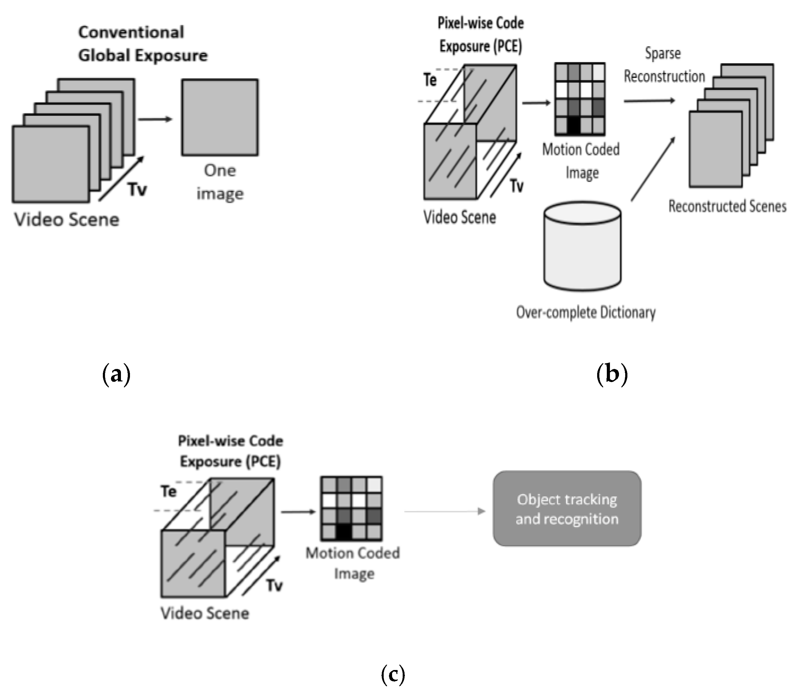
In this paper, we employ a sensing scheme based on PCE or also known as Coded Aperture (CA) video frames as described in [11]. Figure 1 illustrates the differences between a conventional video sensing scheme and PCE, where random spatial pixel activation is combined with fixed temporal exposure duration. First, conventional cameras capture frames at certain frame rates such as 30 frames per second. In contrast, PCE camera captures a compressed frame called motion coded image over a fixed period of time (T_v). For example, a user can compress 30 conventional frames into a single motion coded frame. This will yield significant data compression ratio. Second, the PCE camera allows a user to use different exposure times for different pixel locations. For low lighting regions, more exposure times can be used and for strong light areas, short exposure can be exerted. This will allow high dynamic range. Moreover, power can also be saved via low sampling rate in the data acquisition process. As shown in Figure 1, one conventional approach to using the motion coded images is to apply sparse reconstruction to reconstruct the original frames and this process may be very time consuming.

The coded aperture image $Y\in R^{M\times N}$ is obtained by

$$Y(m,n)={\displaystyle \sum _{t=1}^{T}S(m,n,t)·X(m,n,t)}$$

(1)

where $X\in R^{M\times N\times T}$ contains a video scene with an image size of M $\times$ N and the number of frames of T; $S\in R^{M\times N\times T}$ contains the sensing data cube, which contains the exposure times for pixel located at (m,n,t). The value of S (m,n,t) is 1 for frames t ∈ [t_start, t_end] and 0 otherwise. [t_start, t_end] denotes the start and end frame numbers for a particular pixel. It should be noted that coded exposure is in time domain and coded aperture is in spatial domain. Our proposed PCE imaging actually contains both coded exposure and coded aperture information. This can be seen from Equation (1) above. The elements of the full or a small portion of the sensing data cube in 3-dimensional spatio-temporal space can be activated based on system requirements. Hence, the S matrix contains both coded exposure and coded aperture information. We illustrate the PCE 50% Model in Figure 2 below. In this example, colored dots denote non-zero entries (50% activated pixels being exposed) whereas white part of the spatio-temporal cube are all zero (these pixels are staying dormant). The vertical axis is the time domain, the horizontal axes are the image coordinates, and the reader is reminded that each exposed pixel stays active for an equivalent duration of 4 continuous frames. The “4” is design parameter for controlling exposure times. The larger the exposure times, the more smear the coded image will be in videos with motion.

The video scene $X\in R^{M\times N\times T}$ can be reconstructed via sparsity methods (L₁ or L₀). Details can be found in [11]. However, the reconstruction process is time consuming and hence not suitable for real-time applications.

Instead of performing sparse reconstruction on PCE images, our scheme directly works on the PCE images. Utilizing raw PCE measurements has several challenges. First, moving targets may be smeared if the exposure times are long. Second, there are also missing pixels in the raw measurements because not all pixels are activated during the data collection process. Third, there are much fewer frames in the raw video because a number of original frames are compressed into a single coded frame. This means that the training data will be limited.

In this paper, we have focused on simulating PCE measurements. We then proceed to demonstrate that detection and classifying moving vehicles is feasible. We carried out multiple experiments with two diverse sensing models: PCE/CA Full and PCE/CA 50%. Full means that there are no missing pixels. We also denote this case as 0% missing case. The 50% case means 50% of the pixels in each frame are also missing in the PCE measurements.

The PCE Full Model (PCE Full or CA Full) is quite similar to a conventional video sensor: every pixel in the spatial scene is exposed for exactly the same duration of one second. This simple model still produces a compression ratio of 30:1. The number “30” is a design parameter, which means that 30 frames are averaged to generate a single coded frame. Based on our sponsor’s requirements, in our experiments, we have used 5 frames, which achieved 5 to 1 compression already. More details can also be found in [25,26,27,28,29].

2.2. YOLO

YOLO tracker [30] is fast and has similar performance as Faster R-CNN [31]. We picked YOLO because it is easy to install and is also compatible with our hardware, which seems to have a hard time to install and run Faster R-CNN. The training of YOLO is quite simple. Images with ground truth target locations are needed. YOLO also comes with a classification module.

The input image is resized to 448 × 448. Figure 3 shows the architecture of YOLO version 1. There are 24 convolutional layers and 2 fully connected layers. The output is 7 × 7 × 30.

In contrast to typical detectors that look at multiple locations in an image and return the highest scoring regions as detections, YOLO, as its namesake explains, looks at the entire image to make determinations on detections, giving each scoring global context. This method makes the prediction extremely fast, up to one thousand times faster than an R-CNN. It also works well with our current hardware. It is easy to install, requiring only two steps and few prerequisites. This differs greatly from many other detectors that require a very specific set of prerequisites to run a Caffe based system. YOLO works without the need for a GPU but, if initialized in the configuration file, easily compiles with the Compute Unified Device Architecture (CUDA), which is the NVIDIA toolkit, when constructing the build. YOLO also has a built-in classification module. However, the classification accuracy using YOLO is poor according to our past studies [25,26,27,28,29]. While the poor accuracy may be due to a lack of training data, the created pipeline that feeds input data into YOLO and is therefore more effective at providing results.

One key advantage of YOLO is its speed as it can predict multiple bounding boxes per grid cell of size 7 × 7. For the optimization process during training, YOLO uses sum-squared error between the predictions and the ground truth to calculate loss. The loss function comprises the classification loss, the localization loss (errors between the predicted boundary box and the ground truth), and the confidence loss. More details can be found in [30].

YOLO has its own starter model, Darknet-53, that can be used as a base to further train a given dataset. It contains, as the name would suggest, 53 convolutional layers. It is constructed in a way to optimize speed while also competing with larger convolutional networks.

In the training of YOLO, we trained the models based on missing rates. There may be other deep learning based detectors such as the Single Shot Detector (SSD) [32] in the literature. We tried to use SSD. After some investigations, we observed that it is very difficult to custom trained it. In any event, our key objective is to demonstrate vehicle detection and confirmation using PCE measurements. Any relevant detectors can be used.

2.3. Real-Time System

As shown in Figure 4, the key idea of the proposed system is to use a compressive sensing camera to capture certain scenes. The compressive measurements are wirelessly transmitted to a remote PC for processing. The PC has fast processors such as GPU to carry out the object detection and classification. The processed frames are then wirelessly transmitted to another laptop for display. This scenario is realistic in a sense that there are some applications that can be formalized in the same manner. One application scenario is for border monitoring. A border patrol agent can launch a drone with an onboard camera. Due to limited processing power on the drone, the object detection and classification cannot be done onboard. Instead, the videos are transmitted back to the agent who has a powerful PC, which then processes the videos. The results can be sent back to the control center or the agent for display. Another application is for situation assessment. A soldier at the frontline can sent a small drone with an onboard camera to monitor enemy’s activities. The compressive measurements are sent back to the control center from processing. The processed frames are then sent back to the soldier for display. A third application scenario was also mentioned in Section 1 for search and rescue operations.

2.3.1. Tools Needed

The following tools are needed for real-time processing:

• Ubuntu 16.04 LTS
• Python 2.x
• OpenCV 3.x
• Hamachi
• Haguichi
• TeamViewer

For the operating system, each machine will need to be running on Ubuntu 16.04 LTS and have the following packages installed: Python 2.x, OpenCV 3.x, Hamachi, and Haguichi. This Linux distribution was chosen because it is compatible with the YOLO object detector/classifier. To be consistent, we decided to install the same distribution to each machine.

To run the scripts necessary for the demo, Python and OpenCV are required. The scripts are written in Python and utilizes OpenCV to manipulate the images. Finally, to enable communication between the machines, Hamachi and Haguichi need to be installed on each machine. Hamachi is a free software that allows computers to view other computers connected to the same server, as if they were on the same network. Haguichi is simply a GUI for Hamachi, built for Linux operating systems.

It is highly recommended that TeamViewer is installed on each machine to allow one person to execute the scripts needed. Having one person control each machine eliminates confusion and the need for coordination.

2.3.2. Setup for Each Machine

a. For All Machines

All machines must have an internet connection and be running Haguichi and TeamViewer. In the Haguichi menu, the user should be able to see the status of the other machines connected to the server and they should all be connected.

b. Data Acquisition Machine

This machine needs to be connected to the sensor used for data acquisition via USB. In this case, the sensor used is a Logitech camera.

c. Processing Machine

In the script used for processing, the outgoing IP address need to be changed depending on which machine is the desired receiving machine. In most cases, the IP address will typically stay the same if the same machines are used. Assuming that this machine has YOLO installed and they are fully functional, no further setup is required.

d. Display Machine

This machine does not require any further setup.

2.3.3. General Process of System

The system starts at the data acquisition machine. This machine captures data, via webcam, and condenses N frames into one. As of now, five frames are condensed into one. After the frame has been condensed, sub-sampling is applied to remove x% of pixels. The user is able to specify the percentage before executing the program. Typically, this percentage is 0 or 50%. After the processing is complete, the condensed and subsampled frame is sent to the processing machine via network socket. For test cases where there is more than 0% pixels missing, the image will be resized to half its original size to reduce transmission time.

The processing machine receives this data and decodes it for processing. After extensive investigations, it was determined that using only YOLO, for both detection and classification, is sufficient. This method gives us the fastest real-time results. After all processing, the processed frame is sent to the display machine.

This machine receives the processed data in the same way that the processing machine receives data from the processing machine. The only difference is that the data has not been resized from its original size. Once the data is received, the output is displayed on screen for the user to view the detection and classification results.

It is important to mention that when we send data via network sockets, this method encodes data into a bit stream to send to the receiving machine. The receiving machine will decode this bit stream to obtain the original data.

Below are diagrams to illustrate the flow of this system. The graphical flowchart shown in Figure 5 is a high-level overview of the path the data takes. A camera captures the scene. The video frames are condensed using the PCE principle and wirelessly transmitted to a remote processor with fast GPUs. The processed results are sent to the display device wirelessly. The second flowchart shown in Figure 6 is a more detailed look at the system.

3. Experimental Results

There are several sets of trials spanning several months, various weather conditions, and multiple locations. Various obstacles were present in those trials other than the desired classes such as, pedestrians and other vehicles. All of these factors, whether purposely or through circumstance, were used to develop robust models to work in various different scenarios. This real-time project is unique in that when collecting data to be used for training, we are also in the moment running the collected video through YOLO to generate detection data for testing.

3.1. Performance Metrics

The detection method used when in real-time originally just generated images and videos with bounding boxes and the classification labels above the bounding box. Unfortunately, that did not lend well towards our current method of performance metric generation. As a result, ground truth bounding boxes were manually generated using a program called Yolo mark. Afterwards, a script, used in various other projects, was run to generate bounding boxes and performance metrics. These bounding boxes are generated the same way they would be in real time. The five different performance metrics to quantify the information are: Center Location Error (CLE), Distance Precision at 10 pixels (DP@10), Estimates in Ground Truth (EinGT), mean Area Precision (mAP), and number of frames with detection. These metrics are detailed below:

• Center Location Error (CLE): It is the error between the center of the bounding box and the ground-truth bounding box. Smaller means better. CLE is calculated by measuring the distance between the ground truth center location ($C_{x,gt},C_{y,gt}$) and the detected center location ($C_{x,est},C_{y,est}$). Mathematically, CLE is given by

  $$CLE=\sqrt{{\left(C_{x,est}-C_{x,gt}\right)}^2+{\left(C_{y,est}-C_{y,gt}\right)}^2}$$

  (2)
• Distance Precision (DP): It is the percentage of frames where the centroids of detected bounding boxes are within 10 pixels of the centroid of ground-truth bounding boxes. Close to 1 or 100% indicates good results.
• Estimates in Ground Truth (EinGT): It is the percentage of the frames where the centroids of the detected bounding boxes are inside the ground-truth bounding boxes. It depends on the size of the bounding box and is simply a less strict version of the DP metric. Close to 1 or 100% indicates good results.
• Mean Area Precision (mAP): mAP calculates the amount of area overlap for the estimated and ground truth bounding boxes compared to the total area of the two bounding boxes and returns the result as a value between 0 and 1, with 1 being the perfect overlap. The mAP being used can be computed as

  $$mAP=\frac{AreaofIntersection}{AreaofUnion}$$

  (3)
  As shown in Equation (3), mAP is calculated by taking the area of intersection of the ground truth bounding box and the estimated bounding box, then dividing that area by the union of those two areas.
• Number of frames with detection: This is the total number of frames that have detection.

We used confusion matrices for evaluating vehicle classification performance.

3.2. Videos

We have the following specific training datasets: two in the morning, one around noon time, and two in the afternoon with mixed sunny and cloudy days. There are two scenarios: the Johns Hopkins University (JHU) balcony where a camera was located in the balcony of a building in the Johns Hopkins University (JHU) campus in Montgomery County, Rockville, MD, USA and JHU fire escape which is located in another building in the JHU campus. In each video, there are two moving cars (Toyota Camry and Ford Focus). Each video has a length of 1 to 2 minutes. The numbers of frames in the videos range from 1800 to 3600. Hence, we have 10 videos with about 25,000 frames for training. We manually label the target locations (bounding boxes) in all videos.

There are nine testing different videos used to generate these performance metrics. One is at the JHU balcony. Three were in another, the JHU fire escape (IMG428, IMG429, and IMG430). There are five different live trials that were used for data collection and training of the JHU balcony location where the cars took a figure-8 path (Figure 7) around two circles in front of a parking garage and the entrance to JHU campus. The other location used for training and testing was from a fire escape above the office’s parking lot, where the cars take an oval trip around the lot, and had four live trials. To give a general idea of the path that was taken in for JHU balcony a snapshot will be shown below with a line overlaying the path taken where available. For the fire escape set, it would require multiple images being stitched together to get the whole path so a path overlay will not be included. However, the path is a simple oval. Two cars: Ford Focus and Toyota Camry were used in the experiments.

3.3. Detection Results

Observationally, it was noticed that the 75 percent missing pixel tests performed very poorly for both locations due to too much data loss, while 50 percent performed just well enough to gather metrics and 0 percent operated well enough for metrics. The same deep learning YOLO model is used for both locations because it was trained for both locations.

3.3.1. JHU Balcony Scenario

To train the YOLO, multiple videos were collected with a coded aperture webcam at different dates. Two vehicles (Ford Focus and Toyota Camry) were used in our experiments. The vehicle locations in each frame are manually located and saved. The cropped images are then fed into the YOLO for training.

JHU balcony scenario was captured with a coded aperture webcam in frames and then compiled into a video so it could be tested with the script we have used for various other projects. The script runs detection tests and generates the aforementioned performance metrics.

Table 1. Performance metrics for 0 and 50 percent missing pixels. JHU Balcony scenario.

% Missing	CLE	DP@10	EinGT	mAP	% Detection
0	32.08	0.65	0.66	0.45	70.56
50	23.11	0.73	0.80	0.54	16.48

shows the performance metrics generated for one test video of the JHU balcony.

The metrics show that there is an improvement from the 0% missing case to the 50% missing case. However, there is significantly less detection in the 50% missing case. While the values may be better, the results are based on a much smaller sample which could mean an element of luck is occurring. Upon looking at all tables of performance metrics though it is clear that it is not luck but simply a decreased sample size has fewer bad detections. A decrease in bad detections is convenient for performance metrics but there is a definite value to having many vehicle detections with slightly lower performance as opposed to few vehicle detections with decent to good performance.

Figure 8 and Figure 9 show snapshots of detection results for the JHU balcony scenario (0% missing and 50% missing). The vehicle is Ford Focus. For bot 0% and 50% cases, the green bounding boxes are correctly put around the vehicle.

3.3.2. JHU Fire Escape Scenario

The training of YOLO is similar to the previous case. This scenario is more difficult because the camera was held by one of us and was not mounted on a tripod. Moreover, the camera needed to move in order to follow the vehicles. Consequently, the PCE measurements are blurry and fuzzy caused by the camera motions.

To get a more rounded sense of the performance of the model, the performance metrics tables from each video from the fire escape are provided below in

Table 2. Performance metrics for 0 and 50 percent missing pixels. JHU fire escape scenario: Video IMG428.

IMG428
% Missing	CLE	DP@10	EinGT	mAP	% Detection
0	42.16	0.56	0.94	0.59	84.31
50	15.86	0.62	1.00	0.70	25.49

,

Table 3. Performance metrics for 0 and 50 percent missing pixels. JHU fire escape scenario: Video IMG429.

IMG429
% Missing	CLE	DP@10	EinGT	mAP	% Detection
0	71.36	0.64	0.95	0.63	80.39
50	8.55	0.78	1.00	0.72	33.33

and

Table 4. Performance metrics for 0 and 50 percent missing pixels. JHU fire escape scenario: Video IMG430.

IMG430
% Missing	CLE	DP@10	EinGT	mAP	% Detection
0	113.46	0.68	0.91	0.62	76.47
50	8.97	0.64	1.00	0.76	21.57

. Again, the same pattern emerges, with the 0 missing cases having decent performance in most categories and a large number of detections and the 50 missing cases having good performance but a small number of detections. The water is a little muddier for this set; however, because in Table 4 the 50 missing case has worse performance for DP@10 than the 0 missing case. Not to mention most metrics except for CLE are very close to each other between the two missing pixel cases, having almost negligible differences.

This information shows that the 0 missing pixel cases simply generate false positives, especially because of the large number of other stationary vehicles that skew the metrics. The CLE value is most skewed because it is based off pixel distance from the center location of the ground truth; something that could be greatly skewed by a few bad detections. The other values are less skewed because they are simply percentages that would not be greatly affected by a few bad detections. The 50 missing case would then not have many false vehicle detections because the data from the stationary cars are too obscured to warrant false detections and only the strongest and most clear instances of a class of car triggers a detection. This leads to quite accurate performance metrics. The metric that would most benefit from this style of detection would be CLE as no inaccurate detections would lead to significantly more accurate results. The other metrics meanwhile would only notice a slight increase in accuracy.

For visual inspection of the 0% and 50% missing cases, we only show the snapshots for one of the videos (IMG428) in Figure 10 and Figure 11. There are some missed and false detections due to blurry images. The other two results (IMG429 and IMG430) can be found in the Appendix A.

3.4. Classification Results

The following sets of tables (Table 5 and Table 6) are a snapshot of the classification capabilities of the YOLO deep learning model that was trained. Overall the model does a good job of detecting an object correctly. Instances where a bounding box did not surround a class object were not counted when looking at the set of trials taken from the fire escape. This is because it would be an erroneous measure of the classifiers accuracy. This was not as feasible with the balcony trials, as there were a much larger number of frames. There are instances in that trial set where the number of classifications can equal to a larger number than the total frames of a given video. This simply means that there were multiple detections per frame and on occasion there could be multiple detections of the same classification on the same object. Those instances were not filtered out. The most blatant instance of this will be noticed for the JHU balcony 0 missing pixel trial. That video has 220 frames and yet it has 594 detections averaging to 2.7 detections per frame. A large number of those are simply repeat detections that were unfiltered from the process.

As far as the JHU Balcony trial is concerned, the model is less accurate than the other data set. This makes sense because, unlike the fire escape scenario, the balcony had too many frames to go through to individually confirm which bounding boxes surrounded the actual vehicle to remove the non-vehicle bounding boxes from the results. Knowing this, the model preforms decently well, correctly identifying a Ford Focus 54.7 percent of the time for 0% missing case. It has decreased performance for 50 missing pixels, as expected. For 50 percent missing pixels, the accurate classification percentage is 40.3 percent.

After analyzing the information from the IMG428 trial, it is clear from the above confusion matrices that the YOLO classifier does a pretty decent job of classification. From the data provided, a hypothesis can be generated for the data. It is possible the darker color of the Ford Focus is more clearly detected in higher missing pixel instances as it stands out more clearly from the tarmac it is driving on than the Camry. This pattern continues in the other 50 missing trials. If interested, the other confusion matrices were included in the Appendix A after the tiled images. It also shows that of the 50 frames that are tested the Ford is almost twice as likely to be detected as the Toyota for the 0 missing pixels case. The trend is much more exaggerated for the 50% missing case.

4. Conclusions

Conventional compressive tracking approaches either require tedious image reconstruction or unrealistically assume targets are centered in the images. In this work, we present a real-time framework for vehicle detection and classification directly using compressive measurements collected via pixel-wise code aperture cameras. The PCE camera utilizes a compressive sensing scheme that condenses multiple frames into a code aperture frames and saves power and bandwidth by individually controlling the exposure times of pixels. One key advantage of our proposed approach is that no time-consuming image reconstruction is needed and no assumption of targets in the center of images is required. Hence, real-time target detection and classification has been achieved. Moreover, our approach can handle several practical application scenarios in which the image collection is done using one device with no processing capability, the data processing is done at a second location with fast processors, and the processed results are wirelessly sent over to a device at a third location for real-time visualization. Such scenarios do happen in border monitoring, fire damage assessment, etc. In our experiments, the videos and processed results were all transmitted via a cell phone. The detection and classification is done via YOLO. Real videos were used in our evaluations. In general, the detection is reasonable for 0% and 50% missing cases. However, the classification still needs more improvement.

Currently, we are experimenting with light weight versions of YOLO for detection and classification so that speed can be further improved. We will also explore other detectors such as SSD, which was declared by the authors of SSD [31] to have better performance than YOLO. A third direction is to implement a dynamic scheme to adjust the exposure of each pixel based on the intensity in the image scene.