Article

FlexAlign: An Accurate and Fast Algorithm for Movie Alignment in Cryo-Electron Microscopy

by
David Střelák
1,2,3,*,
Jiří Filipovič
2,
Amaya Jiménez-Moreno
3,
Jose María Carazo
3 and
Carlos Óscar Sánchez Sorzano
3
1
Faculty of Informatics, Masaryk University, Botanická 68a, 60200 Brno, Czech Republic
2
Institute of Computer Science, Masaryk University, Botanická 68a, 60200 Brno, Czech Republic
3
Spanish National Centre for Biotechnology, Spanish National Research Council, Calle Darwin, 3, 28049 Madrid, Spain
*
Author to whom correspondence should be addressed.
Electronics 2020, 9(6), 1040; https://doi.org/10.3390/electronics9061040
Submission received: 14 May 2020 / Revised: 18 June 2020 / Accepted: 18 June 2020 / Published: 23 June 2020
(This article belongs to the Special Issue FPGA/GPU Acceleration of Biomedical Engineering Applications)

Abstract

:
Cryogenic Electron Microscopy (Cryo-EM) has been established as one of the key players in Structural Biology. It can reconstruct a 3D model of the sample at the near-atomic resolution, which led to a Method of the year award by Nature, and the Nobel Prize in 2017. With the growing number of facilities, faster microscopes, and new imaging techniques, new algorithms are needed to process the so-called movies data produced by the microscopes in real-time, while preserving a high resolution and maximum of additional information. In this article, we present a new algorithm used for movie alignment, called FlexAlign. FlexAlign is able to correctly compensate for the shift produced during the movie acquisition on-the-fly, using the current generation of hardware. The algorithm performs a global and elastic local registration of the movie frames using Cross-Correlation and B-spline interpolation for high precision. We show that our execution time is compatible with real-time correction and that we preserve the high-resolution information up to high frequency.

1. Introduction

The processing pipeline of the Cryo-EM consists of several steps, movie alignment being the very first one. A movie is a sequence of frames produced by the microscope, with each frame recording a projection of tens to hundreds of particles. By averaging frames, a micrograph is produced, which is later used for particle picking, Contrast Transfer Function (CTF) estimation, and other steps of the image processing pipeline. Due to beam-induced motion and other changes within the recorded area during the screening, simple averaging of the frames is not sufficient.
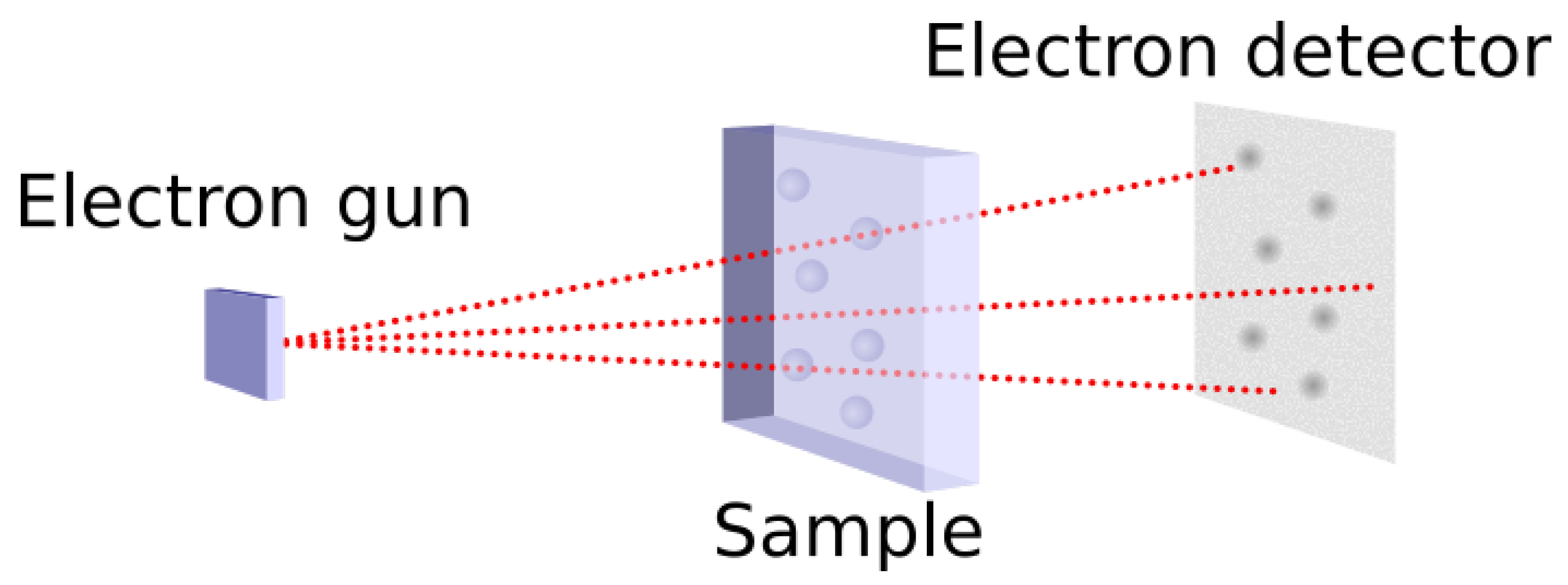
To obtain a single frame, a beam of electrons is fired against the sample. After passing the sample, the beam is recorded by a direct electron detection camera. This is known as Transmission Electron Microscopy (TEM), see Figure 1. Since the electron beam causes radiation damage, the electron dose has to be very low, about one electron per Å 2 and frame (electron arrival is supposed to occur following a Poisson distribution; this means that the most common observations are 0 or 1 electron per pixel). This, on the other hand, results in an extremely low Signal-to-Noise Ratio (SNR). To get more signal, we can repeat the imaging several times using the same sample and then average the resulting frames.
However, before averaging the frames, they have to be properly aligned as the sample moves during the acquisition. The reasons for this movement may vary from sample to sample and they are carefully described by [1]. This movement can be both global and local, and both types need to be corrected.
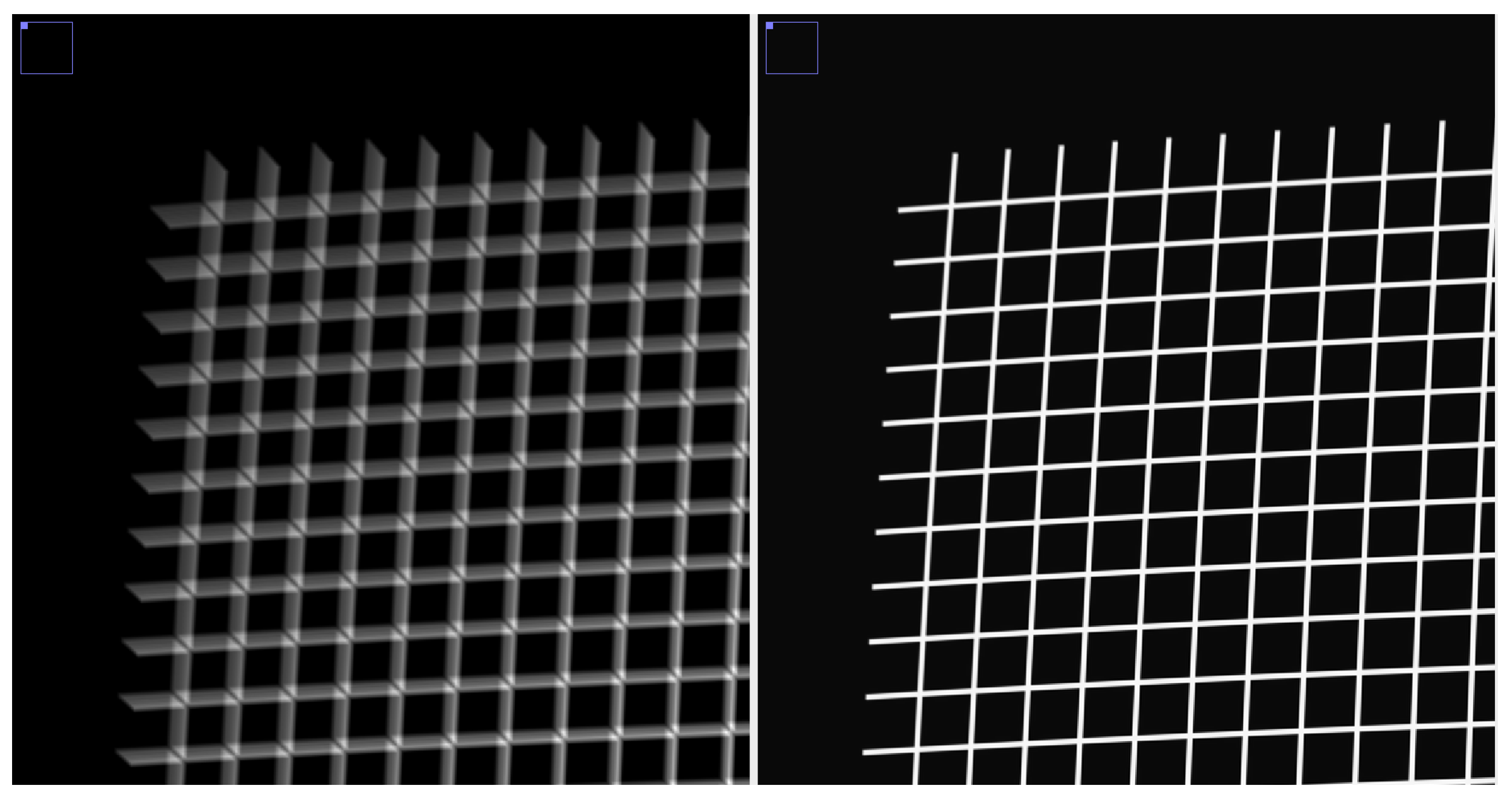
Global alignment is trying to compensate for the apparent movement of the entire frame. Even though this can lead to incorrect alignment at a specific location, the overall SNR will be highly improved. For that reason, it is often used as the first step before local alignment. In Figure 2, we can see the possible effect of (not) performing the global alignment on a noiseless phantom movie, generated and aligned as described in Section 4.1.
The aim of the local alignment is to compensate for more complex movements of the particles, should they be caused by the beam, doming, or another cause. Typically, it works on a divide and conquer basis—the movie is divided into small patches, and the alignment is solved independently for each patch. Figure 3 shows the possible effect of (not) performing the local alignment on a phantom movie.
The requirement for fast and precise algorithms for movie alignment is driven by three factors. The first is speed. The new generation of detectors [2] and acquisition practices reduced the recording time to 4 movies per minute [3], and this time is expected [4] to reach as little as 5 s per movie soon. It is crucial to be able to process these movies in real-time, as potential problems with the imaging can be corrected as soon as they appear during the acquisition (the access cost to the microscope ranges from $1000 to $3000 per day).
The second is accuracy. The goal of Cryo-EM is to produce near-atomic models of the macromolecules under study [5]. This goal sets an important challenge to all the image processing steps, especially this one, as the SNR of the micrographs ranges from 1/10 to 1/100 (At the level of the frame, this SNR has to be divided by the number of frames, typically between 10 and 100.).
The third is particle tracking for polishing. Being able to accurately track the particles back to the originating frames is crucial during the polishing phase, which aims to further improve the resolution of the final 3D reconstruction.
In this article, we introduce a tool for movie alignment called FlexAlign. We give details of our algorithm to perform the movie alignment using the Graphical Processing Unit (GPU) and Compute Unified Device Architecture (CUDA). We propose a two-stage (global and local) movie alignment algorithm based on Cross-Correlation (CC) and B-spline interpolation for the description of the local shifts. As we show, FlexAlign produces high contrast micrographs, it is rather robust to noise, and it is able to process movies at the microscope acquisition speed, using the current generation of the GPUs.
The rest of the paper is organized as follows. Section 2 gives additional details on movie alignment, including the (non) functional requirements of the algorithm. In Section 3, we describe our implementation. Quality and performance evaluation is done in Section 4. Conclusions and future work can be found in Section 5.

Comparison to Other Implementations

Probably the most commonly used SW for movie alignment is currently MotionCor2 [6]. While MotionCor2 provides good performance and precision, it is not providing, to the best of our knowledge, the data needed for particle tracking. It allows for both global and local alignment and is accelerated on GPU. Similarly to our method or the one of Warp [7], it uses CC to align frames or patches of the movie.
The Optical Flow [8] approach can describe the per-pixel movement, but at the cost of high storage requirements—for each pixel of each frame, a 2D shift-vector has to be stored (Provided the shift-vector is stored in single precision, we would need 128 MB per frame of 4000 × 4000 pixels, or 6.25 GB for a movie with 50 frames. Movies are often stored in single-precision, uncompressed format, meaning that the storage requirement would triple.). In addition, the optical flow is computationally expensive, even in a GPU accelerated version.
Relion [9] implements Bayesian polishing, and to expose the metadata of the movie alignment, they provide their Central Processing Unit (CPU) version of the MotionCor2.
The brief overview of the current alignment algorithms can be found in the Table 1.
The goal of FlexAlign is to combine the best of these, namely, the short computational time, the flexibility of elastic deformations, support for detailed pixel tracking, and open-source implementation.

2. Movie Alignment

2.1. Our Method

2.1.1. Global Alignment

For each pair of frames f i and f j (where j > i ), we estimate their apparent shift r ^ i j exploiting the correlation theorem of the Fourier Transformation (FT). Then, we try to find a sequence of shifts between one frame and the next that explains the observed shifts between any pair of frames (see Equation (1)). For doing that, we try to find a unique shift-vector per frame such that the sum of the shifts of all intervening frames r i r j matches the observation:
r i + r i + 1 + + r j 1 = r ^ i j
We get an overdetermined set of linear equations, as the number of unknowns r 1 r n 1 is smaller than the known shifts r ^ i j . It can be expressed in a matrix form as
A r = r ^
The actual per frame movement can be computed by solving Equation (3) in the Least Squares sense
r = ( A T A ) 1 A T r ^
The equation system in Equation (2) may contain outliers due to misestimates of the true shifts between pairs of frames. After solving the equation system, we compute the residuals for each equation and remove those equations whose residual is larger than three standard deviations in absolute value. Then, the equation system is solved again with the remaining equations.
For each frame within the micrograph, we report the global shift parameters. In this way, decisions on the stability of the acquisition process can be quickly taken.

2.1.2. Local Alignment

The local alignment uses a principle similar to the global alignment. We cut each frame into several possibly overlapping rectangular segments (see Figure 4). The equivalent segments in consecutive frames are called patches.
Patches can be handled in the same way as regular movie frames, i.e., we can compute the alignment between them. Once we know the relative shift between all pairs of patches, we can try to fit a smoothing function to this data. We use cubic B-splines, which provide a good trade-off between smoothing quality and computational complexity [10]. Let us refer as r i p = ( r i , x p , r i , y p ) to the shift of the patch p in frame i calculated in the same way as we did for the global alignments. Let us refer as ( x p , y p ) to the coordinate center of the patch p in the coordinate system of the micrograph ( ( 0 , 0 ) is in the top-left corner) before alignment. Then, we look for the B-spline coefficients c l m n , x and c l m n , y such that
r i , x p = l m n c l m n , x B ( i T f l ) B ( x p T x m ) B ( y p T y n )
where B ( · ) is the cubic B-spline function, T f , T x , and T y are the separation between spline nodes in the time, x and y directions, respectively. The equation above should hold for all patches p and frames i. A similar equation applies to c l m n , y . Note that the equation system above is linear in the c coefficients, and we also solve it through the Least Squares problem in which we identify outliers and remove them.
We store the B-spline interpolation c coefficients together with the interpolation nodes geometry ( T f , T x , and T y ), with each micrograph. In that way, we are able to backtrack the movement of each pixel of each frame and allow for particle polishing (that is, a more precise local shift estimation per particle).

2.1.3. Complexity

As can be seen, for the global alignment, our algorithm needs N forward FTs, and N ( N 1 ) 2 inverse FTs, where N is the number of frames. The dimension of the data during the forward FT is typically the original size of the frame, while the size of the inverse FT is usually smaller (Full-scale forward FT is followed by a cropping of the high-frequency data. While downscaling speeds up the transformation, it also improves the precision by suppresing noise.).
The local alignment part needs an additional M N forward FTs and M N ( N 1 ) 2 inverse FTs, where M is the number of segments.
Other operations, such as equation system solving, are negligible in comparison to the total computational demand of the FTs.

3. Implementation

3.1. Alignment Estimation

The pseudocode of the core functionality—alignment estimation of several images (either frames or patches) is shown in Algorithm 1 and Figure 5. As can be seen, for each image, we need to iterate through all consecutive images and compute the relative shift using CC. Ideally, both parts of the algorithm would be executed on GPU, to avoid memory transfer overhead. However, the current generation of GPUs is still manufactured with a rather small amount of on-board memory, which is typically in the range of 6–12 GB on consumer-class cards, and up to 48 GB on professional-class cards.
Algorithm 1 Compute alignment estimation
1:
functioncompute_alignment( i m a g e s ) // frames or patches
2:
     i m a g e s c = { }
3:
    for all i m g i i m a g e s do
4:
         i m g i = F T ( i 1 ) // conversion to FD
5:
        // crop very high frequencies and apply the filter on the rest
6:
         i m g i c = l o w p a s s _ f i l t e r ( i m g i , f i l t e r )
7:
         i m a g e s c . a p p e n d ( i m g i c )
8:
     s o l v e r = e q u a t i o n _ s y s t e m _ s o l v e r ( )
9:
    for all i m g i c i m a g e s c do
10:
        for all i m g j c ( i m g ( i + 1 ) c , i m g n c ) do
11:
            x , y = s h i f t _ a l i g n m e n t ( i m g i c , i m g j c )
12:
            c c = i 1 c · i 2 c // cross-correlation
13:
            c c = I F T ( c c ) // inverse transformation
14:
            x , y = p o s ( m a x ( c c ) ) // position of the maxima is the estimated shift
15:
            s o l v e r . a d d _ e q u a t i o n ( ( i m g i c , i m g j c ) , ( x , y ) )
16:
 
17:
    return s o l v e r . s o l v e ( )
Like other authors, we have used batch processing to overcome this issue. This requires the reorganization of some steps of the algorithm. First, we transfer N images to GPU, perform forward FT, low pass filtering including cropping, and we download the resulting images in the Frequency Domain (FD) to Random Access Memory (RAM) (see Line 7 of Algorithm 1). N is selected such that we have enough space for out-of-place FT, cropped data and the low pass filter. Transfer back to RAM creates natural synchronization/debug point, and allows us to process data even on low-end GPUs, or high-resolution movies with many frames. The pseudocode of this process is shown in Algorithm 2. For simplicity, we skip the boundary and other checks and kernel settings.For filtering, we use standard low-pass Gaussian filter with given maximal resolution. Due to the properties of the Gaussian distribution (99.7% of the values are within three standard deviations from mean.), we know that values at four standard deviations are almost zero, i.e., we can crop out these values completely. The remaining values are multiplied by the weight as given by the distribution. We compute sigma as σ = T s R m a x · 1 2 log 0.5 , where T s is the target resolution in pixels and R m a x is the maximal resolution to preserve in Å.
The following step (of Algorithm 1) is the computation of the CC between images. The pseudocode of this process, without boundary and other checks, is outlined in Algorithms 3 and 4.
Algorithm 2 Batched FT and low-pass filtering
1:
functiontransform_to_FD( i m a g e s , f i l t e r )
2:
    result = {} // cropped and filtered images in FD
3:
     N = f i n d _ b a t c h _ s i z e ( i m a g e s , f i l t e r )
4:
    for i = 0 ; i < | i m a g e s | ; i + = N do
5:
         b a t c h = t r a n s f e r _ t o _ G P U ( i m a g e s , i , i + N )
6:
         b a t c h = F T ( b a t c h ) // conversion to FD
7:
         b a t c h f i l t e r e d = l o w p a s s _ f i l t e r _ k e r n e l ( b a t c h , f i l t e r )
8:
         r e s u l t . a p p e n d ( t r a n s f e r _ f r o m _ G P U ( b a t c h f i l t e r e d ) )
9:
    return r e s u l t
Algorithm 3 Batched shift estimation
1:
functioncompute_shift_estimation( i m a g e s )
2:
    result = {} // cropped correlation centers
3:
     I , J = f i n d _ b u f f e r _ a n d _ b a t c h _ s i z e ( i m a g e s )
4:
    for i = 0 ; i < | i m a g e s | ; i + = I do
5:
         b u f f e r 1 = t r a n s f e r _ t o _ G P U ( i m a g e s , i , i + I )
6:
         r e s u l t . a p p e n d ( b a t c h _ c c ( b u f f e r 1 , b u f f e r 1 , J ) // see Algorithm 4
7:
        for j = i + 1 ; j < | i m a g e s | ; j + = I do
8:
            b u f f e r 2 = t r a n s f e r _ t o _ G P U ( i m a g e s , j , j + I )
9:
            r e s u l t . a p p e n d ( b a t c h _ c c ( b u f f e r 1 , b u f f e r 2 , J ) // see Algorithm 4
10:
 
11:
    return r e s u l t
Algorithm 4 Batched CC
1:
functionbatch_cc( b u f f e r 1 , b u f f e r 2 , b a t c h _ s i z e )
2:
     r e s u l t = { } / / c r o p p e d c o r r e l a t i o n f u n c t i o n s
3:
     n o _ o f _ c c = c o m p u t e _ n u m b e r _ o f _ c o r r e l a t i o n s ( b u f f e r 1 , b u f f e r 2 )
4:
    for i = 0 ; i < n o _ o f _ c c + b a t c h _ s i z e ; i + = b a t c h _ s i z e do
5:
         c c = p o i n t w i s e _ m u l t i p l y _ a n d _ s h i f t _ k e r n e l ( b u f f e r 1 , b u f f e r 2 , i )
6:
         c c = I F T ( c c )
7:
         c e n t e r s = c r o p _ c e n t e r s ( c c )
8:
         r e s u l t . a p p e n d ( t r a n s f e r _ f r o m _ G P U ( c e n t e r s ) )
9:
    return r e s u l t
We use four buffers on the GPU:
  • The first two represent two floating windows, each holding I consecutive images from the previous step.
  • The other two hold results of J pointwise multiplications of the images, in FD and in Spatial Domain (SD) respectively (variables c c and c c on Lines 5 and 6 of the Algorithm 4).
I and J are selected so that they fit into available GPU memory. First, we upload to GPU I images into the first buffer, and another I images to the second buffer. Then, we run a kernel performing pointwise multiplication of all pairs of images in the first buffer, in batch of J images (see the first step in Figure 6). Since we always use images of even size, we also multiply each element of the resulting image by 1 ( i + j ) , where i , j are positions of each element. After inverse FT, this results in shifting the correlation function to the center of the image. The last step is to crop the correlation centers and download them to RAM for further processing.
Similarly, we get centers of correlations between images in the buffers, see the second step in Figure 6. We keep loading consecutive images to the second buffer until we pass through all of them, as shown in step three in Figure 6. Once that happens, we upload new images also to the first buffer and repeat the process until all pairs of images are processed.
To locate the position of the maxima, we use sub-pixel averaging. We locate the pixel with maximal value. From it, we search for the nearest pixel with value m a x / 2 . Distance to this pixel determines an area, in which we do a weighted average of the pixels. The position of this average is the requested shift. Due to a complicated memory access pattern and low exposed parallelism, we kept this code on the CPU side. The obtained positions of the maxima, i.e., relative shifts of all pairs of frames, are used as input to the linear equation system solver, as described in Section 2.1.1.

3.2. Global Alignment

Our algorithm starts by loading all frames into a consecutive block of RAM. During the load, we also apply a gain and dark image correction (A dark image is a residual signal generated by the sensor when no electrons are fired at it, and a gain image corrects uneven sensitivity of the sensor’s pixels.), if requested. Then, we apply a low pass filter and estimate the shifts of all frames, as described in the previous subsection.

3.3. Local Alignment

Local alignment is a direct extension of the global alignment. We use the fact that we already have frames loaded in RAM. We process the frames by segments—we copy out proper patches, and at the same time, we compensate for the global shift estimated in the previous step. Since patches are typically smaller than frames, we average data from several (three, by default) frames together, to suppress the noise and enhance the signal. As typical particle has size of 200–300 Å, we use by default patches of 500 × 500 Å, so that at least one particle can fit in it.
Once extracted, patches are then handled in the same fashion as frames of the global alignment. The pseudocode without frame averaging is shown in Algorithm 5.
Algorithm 5 Local movie alignment
1:
functionlocal_alignment( f r a m e s )
2:
     g l o b a l _ s h i f t = c o m p u t e _ a l i g n m e n t ( f r a m e s )
3:
     p a t c h _ s h i f t s = { } // absolute shift of each patch
4:
    for all s s e g m e n t s do
5:
         s o l v e r = e q u a t i o n _ s y s t e m _ s o l v e r ( )
6:
         p a t c h e s = e x t r a c t _ p a t c h e s _ f r o m _ f r a m e s ( f r a m e s , g l o b a l _ s h i f t , s )
7:
         p a t c h e s _ s h i f t s = c o m p u t e _ a l i g n m e n t ( p a t c h e s )
8:
         s o l v e r . a d d _ e q u a t i o n s ( p a t c h e s , p a t c h e s _ s h i f t s )
9:
         p a t c h _ s h i f t s . a p p e n d ( s , s o l v e r . s o l v e ( ) )
10:
    return p a t c h _ s h i f t s

3.4. CuFFTAdvisor

As can be seen from the text above and Section 2.1.3, our method is strongly dependent on the performance of the FT.
We use the standard NVIDIA’s cuFFT library [11]. As the performance and additional memory consumption of this library depend on the size of the input data and type of the transformation, we have developed custom software, cuFFTAdvisor [12] that uses autotuning to help us to automatically determine the best settings.
During the global alignment, we search for the size of the frame, which could be up to 10% smaller and is faster to process. This can also result in up to 8 times less space used by the library itself, see [12] for details.
As stated earlier, during filtering, we crop high frequencies (over four standard deviations) of the frames in the FD. We autotune for the sizes which could be up to 10% bigger, but faster to process. Once we know this size, we simply have to alter the filter to take this size change into account.
Sizes of the (filtered) patches during the local alignment are obtained in a similar fashion.
To compensate for the time spent on autotuning, we store the autotuned sizes in a user-defined file as key-value pairs. As key, we use a combination of the GPU used, input size of the movie, and available GPU memory. The value is, then, the optimized size.
Users can also opt-out of this autotuning step, should it lead to overall slow-down, e.g., during the processing of a few movies only.

4. Quality and Performance Analysis

To ensure that our algorithm is able to cope with complex movements and noise, we have run a collection of tests.

4.1. Phantom

First, we have generated a phantom movie, consisting of 30 frames of 4096 × 4096 pixels. Each frame contains a grid of 5 pixels wide lines 50 pixels apart. Grid pixels were set to one, background ones to zero. Each pixel [ x , y ] of each frame t has been shifted using the following formulas:
x ( t ) = a 1 ( n t ) + a 2 ( n t ) 2 + c o s ( n t ) / 10 y ( t ) = b 1 ( n t ) + b 2 ( n t ) 2 + s i n ( ( n t ) 2 ) / 5
After the shift, a doming has been applied, with the center of the doming located in the middle of the frame, using the normalized distance r from it:
k 1 = k 1 s + t ( k 1 e k 1 s ) / n k 2 = k 2 s + t ( k 2 e k 2 s ) / n r o u t = r i n ( 1 + k 1 r i n 2 + k 2 r i n 4 )
where r o u t and r i n are the radial coordinate of the pixel in the output and input images, respectively.
We have used the following constants: n = 30 ; a 1 = 0.039 ; a 2 = 0.002 ; b 1 = 0.02 ; b 2 = 0.002 ; k 1 s = 0.04 ; k 1 e = 0.05 ; k 2 s = 0.02 ; k 2 e = 0.025 and bilinear interpolation between pixels.
We got a phantom movie with a grid, which has both translation and doming applied between each frame. We used this phantom to simulate the image acquisition process in the electron microscope as follows. For each pixel value v, we simulate the arrival of i electrons using a Poisson distribution whose average is controlled by the corresponding phantom pixel:
μ = μ b ( μ b μ f ) v P ( i | μ ) = e μ μ i i !
We used values μ b = 1.25 for background pixels and μ f = 1.05 for foreground (grid) pixels.
Using this phantom, we have tested FlexAlign, MotionCor2 v.1.3.1, Warp 1.07W, cryoSPARC v2.15 (patch_motion_correction_multi) [13] and Relion’s MotionCor v.3.0.8. We have used 9 × 9 segments per frame of 500 × 500 pixels (assumed pixel size = 1.0). CryoSPARC sets the number of segments to 7 × 7 and does not allow for manual override. As can be seen in Figure 7, both MotionCor2 and FlexAlign were able to correct combined shifts correctly, FlexAlign producing a higher contrast micrograph. High contrast is important especially during the picking stage, where it allows for more reliable particle selection, and also could indicate better high-frequency preservation. The other three programs were not able to correct for the shift near the corner of the resulting micrograph. While Relion MotionCor and cryoSPARC get gradually worse, Warp produces a sharper transition.

4.2. Real Movies

We have run similar tests on experimental data. We used the EMPIAR data sets 10288 [14], 10314 [15] and 10196 [16].

4.2.1. EMPIAR 10288

The EMPIAR 10288 dataset consists of movies of 40 frames, each frame having a resolution of 3838 × 3710 pixels. The pixel size is 0.86 Å, which resulted in 9 × 9 patches. The average exposure and the camera model is not specified. Gain correction images are provided for a subset of the movies.
Figure 8 shows a trace of the reported global alignment and histogram of the first frame. As we can see, all programs report very similar shifts, except Warp, which reports around two pixels shorter track. It is worth mentioning that this might be compensated during the local alignment step.
Details of the obtained micrographs are shown in Figure 9. All programs produce relatively sharp micrographs. We can see that MotionCor2 clamps low values a little.
Figure 10 shows the radial average of the Power Spectrum Density (PSD) for the resulting micrographs. As can be seen, micrographs contain useful information up to a resolution between 4 to 5 Å. The power increase at high frequencies of MotionCor2 might indicate some high frequency enhancement, while decreasing tendency of the FlexAlign, Warp, and Relion MotionCor suggest dampening of the high frequencies.

4.2.2. EMPIAR 10314

The EMPIAR 10314 dataset consists of movies of 33 frames, each frame having a resolution of 4096 × 4096 pixels and an average exposure of 1.51 e / Å 2 . The pixel size is 1.12 Å, so we have used 8 × 8 patches. The camera model is not specified and neither gain nor dark correction images are provided. For Warp, the movie has been converted from original .tif format with AdobeDeflate compression to .mrc, as the former is not yet supported.
Figure 11 shows a trace of the reported global alignment and histogram of the first frame. As we can see from the histogram, movie frames have probably been somehow post-processed. For that reason, FlexAlign in default settings (FlexAlign 30 Å) reports a different shift in the x-direction, compared to other programs. However, the difference is rather small, around 1.2 Å on the span of the whole movie. It is interesting that the total shift in the y-direction is over 8 times higher than in the x-direction. If we change the filtering to 10 Å, FlexAlign (FlexAlign 10 Å) results in a global trajectory that is consistent with other algorithms. This experiment highlights the need for the lowpass filter during the calculation of the relative shifts: it is primarily aimed at making sure that the signal being correlated has enough information (remind that normally more than half of the pixels of the frames have no electron hit, and for a typical dose in an area of 30 Å 2 there are about 450 pixels hit by electrons); if the frame already has enough local information (as in this example), it is best not to blur it.
Details of the obtained micrographs are shown in Figure 12. All programs produce sharp micrographs, without any cropping of the high/low values.
Figure 13 shows the radial average of the PSD for the resulting micrographs. These micrographs contain frequencies of up to three and a half Å. Again, MotionCor2’s PSD might indicate problem with handling high frequencies, while decreasing tendency of the cryoSPARC, FlexAlign, Relion MotionCor and Warp suggests dampening of the high frequencies (either by the movie alignment algorithm, the image interpolation scheme to produce the micrograph, or as originally recorded by the movie). Warp dampens the most, followed by Relion MotionCor, FlexAlign and cryoSPARC. CryoSPARC, FlexAlign, Warp, and Relion MotionCor also seem to preserve bit higher frequencies than MotionCor2.

4.2.3. EMPIAR 10196

The EMPIAR 101096 dataset consists of movies of 40 frames, each with a size of 7420 × 7676 pixels and an average exposure of 1.264 e / Å 2 . The pixel size is 0.745 Å (super-resolution) and we used 20 × 21 patches. CryoSPARC used 9 × 10 patches. The camera model is a K2 on a Talos Arctica. Gain is provided along with instructions on application (must be rotated 90 degrees left and flipped horizontally). Figure 14 shows a trace of the reported global alignment and histogram of the first frame. Despite all efforts, we were not able to align this movie with Warp (we were getting zero shift for all frames).
From the reported global shift, we can see that it has an unusually high drift of almost 80 pixels. FlexAlign in default settings checks for shifts of up to 40 pixels (FlexAlign max shift 40) and therefore reports different values as compared to both Relion MotionCor and MotionCor2. This error is partially compensated during the local alignment phase, which is able to compensate for an additional 40-pixel shift. If we allow for higher shifts, FlexAlign (FlexAlign max shift 80) reports similar trace to other algorithms. Details of the obtained micrographs are shown in Figure 15. Again, we can see that MotionCor2 crops the low values. It is worth noticing the difference at the edges of the micrograph—programs handle them differently, and particles coming from these areas should not be used for further steps.
Figure 16 shows the radial average of the PSD for the resulting micrographs. These micrographs contain very low frequencies, below 10 Å, and as such, they might be considered for discarding. Again, MotionCor2’s PSD has increasing tendency, while FlexAlign and Relion MotionCor show decreasing tendency. Similarly to dataset 10288, cryoSPARC does not seem to increase nor decrease the frequencies.

4.2.4. Number of Patches

In the aforementioned tests, we have automatically set the number of segments/patches that are used by FlexAlign during the local alignment estimation, based on the pixel size and the resolution of the frames. By default, we use patches of 500 × 500 Å that we equally distribute to fully cover the frames, i.e., per dimension we use n = R f / R p patches, where R f is resolution of the frame in Å and R p is resolution of the patch in Å. The first and the last patch are aligned with the edges of the frame, and the rest is equally distributed between them.
Figure 17 shows a 10× magnified estimated total (local + global) shift in the grid of 200 × 100 px, using the Covid-19 spike movie we helped to process. The movie consists of 30 frames of 5760 × 4092 pixels, and pixel size of 1.047 Å per pixel. For this resolution, we would use 12 × 8 patches. As can be seen, even four times fewer patches can give us a general idea of the shift in different parts of the movie. Our default value seems to capture all major deviations. Twice as many patches give us even more detailed insight, but might result in overfitting (see the bottom of the last figure), and as such we believe that it is not necessary during this stage of the processing pipeline. It is also worth noticing that the entire first half of the frames move much more than the second half, while the literature generally mentions a big drift of only the first few frames.
We have also tried a different number of patches for MotionCor2 with our phantom movie. As shown in Figure 18, 5 × 5 patches (The default value when used via Scipion.) are not sufficient to compensate the shift, while 9 × 9 (our default value) result in sharp edges. Neither MotionCor2 nor Relion MotionCor offers an automatic patch size setting, so we used the same values as used by FlexAlign throughout the testing. CryoSPARC does not allow for a manual set of the number of patches.

4.3. Performance

We have compared the performance of the FlexAlign, Warp, and MotionCor2 using three machines, as described in Table 2. Relion MotionCor is CPU only and therefore skipped, as well as cryoSPARC, which cannot be set with the same settings. As we could not install MS Windows on the Testbeds 1 and 2, we have compared Warp and FlexAlign using different machines. These results should be taken as illustrative only.
We have tested the most common sizes of the movies, with the default settings for each program, with exception to the number of patches, which was set the same for both programs. The resolution used and the name of the direct detection camera using such a resolution are shown in Table 3. Each configuration has been run five times, and we present the average of these values.
As discussed in Section 3.4, we dynamically change the size of the patches and frames to speed up the processing. For FlexAlign, we have therefore measured the time without autotuning, with autotuning, and after autotuning, when the new sizes are loaded from the local storage. Since autotuning slows down only the first execution, we also report the minimal number of movies necessary to compensate for this extra time. Results can be found in Table 4 for Testbed 1, Table 5 for Testbed 2, and Table 6 for Testbed 3, where we show Warp and tuned times of FlexAlign only for brevity.
As can be seen, MotionCor2 is very well optimized for all tested sizes and GPU architectures. FlexAlign is on average at 63% of its performance after autotuning (51% without autotuning), but both programs are able to process the movies on-the-fly.
In terms of autotuning, it is more important for less powerful GPU, where it pays-off after as few as 6 movies (13 on average). For high-end GPU, at least 20 movies have to be processed (on average) to compensate for the time spent on autotuning. Since typically hundreds to thousands of movies are processed, we use autotuning by default.

5. Conclusions

In this paper, we have presented our new program for movie alignment, called FlexAlign. FlexAlign is a GPU accelerated program able to correct both the global and local shifts of the movies. Using current generations of GPUs, our program is able to process the most common sizes of the movies on-the-fly, though it is slower than its direct competitor, MotionCor2. Compared to MotionCor2, FlexAlign produces micrographs with higher contrast, and it seems to be more resilient to noise than both MotionCor2 and Relion MotionCor. It also tends to preserve higher frequencies in the resulting micrograph. Last but not least, FlexAlign stores the data necessary to track the particle movement with each micrograph to allow for precise particle polishing, in a compact way of the B-spline coefficients.
In future releases, we plan to address several bottlenecks that we have identified in our current implementation, and also to use the information on the local shift during the particle picking and polishing.
FlexAlign is implemented in Xmipp [17], an open-source suite of Cryo-EM algorithms available under GNU General Public License. As part of Xmipp, it is also freely available in the Scipion [18] framework.

Author Contributions

Methodology: J.F. and C.Ó.S.S.; Software: D.S. and A.J.-M.; Text: D.S.; Supervision: J.M.C. All authors have read and agreed to the published version of the manuscript.

Funding

The authors would like to acknowledge financial support from: the Comunidad de Madrid through grant CAM (S2017/BMD-3817), the Spanish Ministry of Economy and Competitiveness (BIO2016-76400-R), the Instituto de Salud Carlos III, PT17/0009/0010 (ISCIII-SGEFI/ERDF) and the European Union and Horizon 2020 through grant: CORBEL (INFRADEV-01-2014-1, Proposal 654248), INSTRUCT-ULTRA (INFRADEV-03-016-2017, Proposal 731005), EOSC Life (INFRAEOSC-04-2018, Proposal: 824087) and HighResCells (ERC-2018-SyG, Proposal: 810057). The project that gave rise to these results received the support of a fellowship from “la Caixa” Foundation (ID 100010434). The fellowship code is LCF/BQ/DI18/11660021. This project has received funding from the European Union’s Horizon 2020 research and innovation programme under the Marie Skłodowska-Curie grant agreement No. 713673. The work was supported from European Regional Development Fund-Project “CERIT Scientific Cloud” (No. CZ.02.1.01/0.0/0.0/16_013/0001802).

Acknowledgments

The authors acknowledge the support and the use of resources of Instruct, a Landmark ESFRI project.

Conflicts of Interest

The authors declare no conflict of interest.

References

  1. Glaeser, R. Methods in Enzymology; Academic Press: Cambridge, MA, USA, 2016; Volume 579, pp. 19–50. [Google Scholar] [CrossRef]
  2. Hattne, J.; Martynowycz, M.W.; Penczek, P.A.; Gonen, T. MicroED with the Falcon III direct electron detector. IUCrJ 2019, 6, 921–926. [Google Scholar] [CrossRef] [PubMed] [Green Version]
  3. Borgnia, M.J.; Bartesaghi, A. Practices in Data Management to Significantly Reduce Costs in Cryo-EM. Microsc. Microanal. 2019, 25, 1378–1379. [Google Scholar] [CrossRef] [Green Version]
  4. Danev, R.; Yanagisawa, H.; Kikkawa, M. Cryo-Electron Microscopy Methodology: Current Aspects and Future Directions. Trends Biochem. Sci. 2019, 44, 837–848. [Google Scholar] [CrossRef] [PubMed]
  5. Marko, A. CryoEM Takes Center Stage: How Compute, Storage, and Networking Needs are Growing with CryoEM Research. 2019. Available online: https://www.microway.com/hpc-tech-tips/cryoem-takes-center-stage-how-compute-storage-networking-needs-growing (accessed on 22 June 2020).
  6. Zheng, S.Q.; Palovcak, E.; Armache, J.P.; Verba, K.A.; Cheng, Y.; Agard, D.A. MotionCor2: Anisotropic correction of beam-induced motion for improved cryo-electron microscopy. Nat. Methods 2017, 14, 331–332. [Google Scholar] [CrossRef] [PubMed] [Green Version]
  7. Tegunov, D.; Cramer, P. Real-time cryo-electron microscopy data preprocessing with Warp. Nat. Methods 2019, 16, 1146–1152. [Google Scholar] [CrossRef] [PubMed]
  8. Abrishami, V.; Vargas, J.; Li, X.; Cheng, Y.; Marabini, R.; Sorzano, C.Ó.S.; Carazo, J.M. Alignment of direct detection device micrographs using a robust optical flow approach. J. Struct. Biol. 2015, 189, 163–176. [Google Scholar] [CrossRef] [PubMed]
  9. Zivanov, J.; Nakane, T.; Forsberg, B.O.; Kimanius, D.; Hagen, W.J.; Lindahl, E.; Scheres, S.H. New tools for automated high-resolution cryo-EM structure determination in RELION-3. Elife 2018, 7, e42166. [Google Scholar] [CrossRef] [PubMed]
  10. Jonic, S.; Sanchez Sorzano, C.O. Optical and Digital Image Processing: Fundamentals and Applications; John Wiley & Sons, Ltd.: Hoboken, NJ, USA, 2011; Chapter 6; pp. 119–134. [Google Scholar] [CrossRef]
  11. NVIDIA. CUFFT Library User’s Guide; NVIDIA: Santa Clara, CA, USA, 2019. [Google Scholar]
  12. Střelák, D.; Filipovič, J. Performance Analysis and Autotuning Setup of the CuFFT Library. In Proceedings of the 2nd Workshop on AutotuniNg and ADaptivity AppRoaches for Energy Efficient HPC Systems, Limassol, Cyprus, 4 November 2018. [Google Scholar] [CrossRef]
  13. Punjani, A.; Rubinstein, J.L.; Fleet, D.J.; Brubaker, M.A. cryoSPARC: Algorithms for rapid unsupervised cryo-EM structure determination. Nat. Methods 2017, 14, 290–296. [Google Scholar] [CrossRef] [PubMed]
  14. Krishna, K.K.; Shalev-Benami, M.; Robertson, M.; Hu, H.; Banister, S.; Hollingsworth, S.; Latorraca, N.; Kato, H.; Hilger, D.; Maeda, S.; et al. Cryo Electron Microscopy of Cannabinoid Receptor 1-G Protein Complex; EMBL-EBI: Cambridgeshire, UK, 2019. [Google Scholar] [CrossRef]
  15. Suga, M.; Ozawa, S.; Yoshida-Motomura, K.; Akita, F.; Miyazaki, N.; Takahashi, Y. Structure of the green algal photosystem I supercomplex with a decameric light-harvesting complex I. Nat. Plants 2019, 5, 626–636. [Google Scholar] [CrossRef] [PubMed]
  16. Nureki, O.; Kasuya, G.; Nakane, T.; Yokoyama, T.; Jia, Y.; Inoue, M.; Watanabe, K.; Nakamura, R.; Nishizawa, T.; Kusakizako, T.; et al. Cryo-EM structures of the human volume-regulated anion channel LRRC8. Nat. Struct. Mol. Biol. 2018, 25, 797–804. [Google Scholar] [CrossRef]
  17. De la Rosa-Trevín, J.; Otón, J.; Marabini, R.; Zaldivar, A.; Vargas, J.; Carazo, J.; Sorzano, C. Xmipp 3.0: An improved software suite for image processing in electron microscopy. J. Struct. Biol. 2013, 184, 321–328. [Google Scholar] [CrossRef] [PubMed]
  18. De la Rosa-Trevín, J.; Quintana, A.; Del Cano, L.; Zaldivar, A.; Foche, I.; Gutiérrez, J.; Gómez-Blanco, J.; Burguet-Castell, J.; Cuenca-Alba, J.; Abrishami, V.; et al. Scipion: A software framework toward integration, reproducibility and validation in 3D electron microscopy. J. Struct. Biol. 2016, 195, 93–99. [Google Scholar] [CrossRef] [PubMed] [Green Version]
Figure 1. Principle of the TEM.
Electronics 09 01040 g001
Figure 2. Phantom movie (grid, detail), an average of 10 frames, nth frame shifted by the vector [ 2 n , 3 n ] , before global alignment (left), after global alignment (right).
Electronics 09 01040 g002
Figure 3. Phantom movie (grid, detail), an average of 50 frames, frames shifted + doming applied, using only global alignment (left), after local alignment (right).
Electronics 09 01040 g003
Figure 4. Division of the frames to patches for local alignment.
Electronics 09 01040 g004
Figure 5. Flowchart of the core idea of the algorithm. Algorithm overview (left), alignment subroutine (right).
Electronics 09 01040 g005
Figure 6. Data processing using two buffers. First, we process images in the first (red) buffer (1), then all pairs of images in both buffers (2). We iteratively fill the second (green) buffer with remaining images (3, arrows skipped for brevity). When all images pairs for the first buffer are processed, we load new images into the first buffer (4).
Electronics 09 01040 g006
Figure 7. Detail of the frame of the phantom movie (top left), detail of produced micrograph, normalized: cryoSPARC (top right), FlexAlign (center left), Warp (center right), MotionCor2 (bottom left), Relion MotionCor (bottom right).
Electronics 09 01040 g007
Figure 8. Detail of the frame from the EMPIAR 10288 (normalized) with histogram (before normalization) (top), reported global shifts by different programs (bottom).
Electronics 09 01040 g008
Figure 9. Detail of the produced micrograph using EMPIAR 10288 dataset (normalized) with histogram (before normalization): FlexAlign (top left), Warp (top right), cryoSPARC (center), MotionCor2 (bottom left), Relion MotionCor (bottom right).
Electronics 09 01040 g009
Figure 10. Radial average of the PSD of the produced micrograph using EMPIAR 10288.
Electronics 09 01040 g010
Figure 11. Details of the frame from the EMPIAR 10314 (normalized) with histogram (before normalization) (top), reported global shifts by different programs (bottom).
Electronics 09 01040 g011
Figure 12. Details of the produced micrograph using EMPIAR 10314 dataset (normalized) with histogram (before normalization): FlexAlign (top left), FlexAlign with low-pass filter at 10 Å (top right), Warp (center left), cryoSPARC (center right), MotionCor2 (bottom left), Relion MotionCor (bottom right).
Electronics 09 01040 g012
Figure 13. Radial average of the PSD of the produced micrograph using EMPIAR 10314.
Electronics 09 01040 g013
Figure 14. Details of the frame from the EMPIAR 10196 (normalized) with histogram (before normalization) (top), reported global shifts by different programs (bottom).
Electronics 09 01040 g014
Figure 15. Details of the produced micrograph using EMPIAR 10196 dataset (normalized) with histogram (before normalization): FlexAlign (top left), FlexAlign with max shift of 80 px (top right), cryoSPARC (center), MotionCor2 (bottom left), Relion MotionCor (bottom right).
Electronics 09 01040 g015
Figure 16. Radial average of the PSD of the produced micrograph using EMPIAR 10196.
Electronics 09 01040 g016
Figure 17. Influence on shift estimation using a different number of patches: 3 × 2 (top), 12 × 8 (middle, default value), 24 × 16 (bottom).
Electronics 09 01040 g017
Figure 18. Normalized micrograph of the phantom movie produced by MotionCor2, using different number of patches: 5 × 5 (left), 7 × 7 (middle), 9 × 9 (right).
Electronics 09 01040 g018
Table 1. Comparison of various movie alignment algorithms.
ProgramHWMethod + Interpolation
MotionCor2GPUCC + polynomial
Relion MotionCorCPUCC + polynomial
Optical flowCPU/GPUoptical flow + cubic interpolation
WarpGPUCC + higher-order schemes
FlexAlignGPUCC + B-spline
Table 2. HW used for benchmarking.
Testbed 1Testbed 2Testbed 3
CPUIntel(R) Core(TM) i7-8700 (12 cores, 3.20 GHz)Intel(R) Core(TM) i7-7700HQ (4 cores, 2.80 GHz)
GPUGeForce RTX 2080GeForce GTX 1070GeForce GTX 1060
CUDA/driver10.1/418.3910.1/418.678.0.61/436.02 (Win 10)/390.116 (Ubuntu 18.04)
SSDSamsung SSD 970 EVO 500 GBNVMe TOSHIBA 1024 GB
RAM2 × 16 GB DDR4 @ 2.6 GHz2 × 16 GB DDR4 @ 2.4 GHz
Table 3. Resolution and number of frames used for testing.
SizeNo. of Patches
Falcon4096 × 4096 × 409 × 9
K23838 × 3710 × 408 × 8
K2 super (resolution)7676 × 7420 × 4016 × 15
K35760 × 4092 × 3012 × 9
K3 super (resolution)11,520 × 8184 × 2024 × 17
Table 4. Execution time on Testbed 1.
FalconK2K2 SuperK3K3 Super
MotionCor24.6 s4.3 s15.7 s5.0 s13.1 s
FlexAlign (tuned)9.2 s7.6 s25.6 s8.8 s20.5 s
FlexAlign (autotuning)49.2 s34.4 s71.9 s59.3 s72.2 s
FlexAlign (non-tuned)10.8 s9.1 s31.5 s10.7 s22.9 s
Movies to pay-off251882722
Table 5. Execution time on Testbed 2.
FalconK2K2 SuperK3K3 Super
MotionCor25.5 s5.2 s20.3 s5.9 s15.7 s
FlexAlign (tuned)9.0 s8.2 s27.3 s9.3 s21.1 s
FlexAlign (autotuning)47.8 s38.7 s73.3 s56.2 s65.7 s
FlexAlign (non-tuned)11.7 s10.4 s35.2 s11.5 s26.9 s
Movies to pay-off15146228
Table 6. Execution time on Testbed 3.
FalconK2K2 SuperK3K3 Super
Warp11.7 s10 s14.2 s13.1 s15.6 s
FlexAlign (tuned)11.9 s9.9 s35.5 s11.3 s27.7 s