1. Introduction
Tracking animals in the wild has gained momentum, and the advancements in technology and the Internet of Things (IoT) have challenged scientists and engineers to design, build, and create devices that outperform predecessors. There are cases where animals are tracked through stationary nodes, but in such cases, the technology heavily depends on the animal being present at a particular location. Others use wireless sensors and technologies that heavily depend on a large power source. These designs include technology that is bulky and power inefficient. The main reason such technology is bulky is due to the batteries used. In some cases, the battery is the bulkiest component of the design [
1]. Other devices rely on wireless technology that is power inefficient, and battery degradation happens withing hours and the harvested energy is consumed quickly. For example, in Ghazali’s et al. [
2] tracking system the battery voltage dropped by more than 20% within an hour. Additionally, several of these technologies and applications lack a network with data collection capability between wireless nodes. The devices are capable of tracking the physical location of an animal but cannot collect data that pertains to the behavior of a species. Many times the behaviors examined are solely based on the physical migration of a particular species. The behavior tracked pertains to a group of species as a whole but never the behavior that corresponds to interactions between individuals in those groups. Similarly, a few companies, such as Lotek [
3], Sigfox [
4], and Telemetry [
5], are producing wearable or implantable devices for animal monitoring and tracking.
In this study, we specifically targeted chimpanzees, one of humans’ closest living relatives [
6], to understand their social behavior. They live in large social groups, up to more than a hundred individuals, with various group dynamics that result in different daily behavior [
7]—splitting during the day, foraging, etc. These relationships can be cooperative, exploitative, or competitive, so can be seen as resembling to human cultures [
8]. The behavior of each individual is deeply affected by their relationship with others in the group, and relationships are usually measured in terms of the proximity of different individuals over time [
9]. Thus, automated behavioral monitoring of chimpanzees has very high potential for understanding the social dynamics of a chimpanzee group. These dynamics are traditionally studied manually by the scientists, which is labor-intensive and time-consuming. This is because in this method, the scientists manually identify the chimpanzees, follow them, and record their behaviors over time. Because of this manual, labor-intensive workload, it becomes very difficult to capture all interactions among the individuals. Thus, an automated solution can significantly improve the efficiency of this process.
Although other technological tracking studies or products are available in the literature or the market, they are not best-suited for our target of automatically understanding the relationships in a chimpanzee group for multiple reasons: (1) These solutions are mostly GPS-based (where a GPS unit is known to be power-hungry and we cannot use it for behavior tracking that requires frequent data collection); (2) These solutions are usually designed for less intelligent or capable animals (such as fish, cows, etc.), thus the designs are quite simplistic, not considering behavior dynamics or the possibility that the animals can take them off; (3) The devices require communication with or through a central device (e.g., a local gateway, a server connected to the Internet or a satellite in the case of GPS), and thus the individual devices would not necessarily have the capability to communicate among each other (i.e., peer-to-peer).
Instead, we propose to develop a device that uses Bluetooth Low Energy (BLE) to facilitate an ad-hoc mesh network among the individuals. We believe that our proposed method to track wildlife can introduce a new and efficient way to track chimpanzees in their natural habitat to obtain information about their social interactions. Since we are interested in group dynamics, which requires proximity, our focus is not to track the actual physical location, but rather track social behavior within a group of a species, which can be measured by physical proximity. We want to know how often they are together and participate in activities together. To that end, we are taking an animal-in-the-loop approach, introduced in [
10,
11], where the technology considers the movements and physical characteristics of the animal that is being monitored. Next, we explore different technological approaches for wildlife tracking and address their trade-offs with respect to our application. At the end of this section, we discuss the limitations of the existing methods, and include comparisons of their operational efficiency and effectiveness, if applicable, to our application.
4. Our Solution for Proximity-Based Wildlife Monitoring
Our design consist of a wireless sensor node that is mobile; therefore, we require a battery as the main power source. Batteries have finite lifetimes; thus, our wireless sensor node also has a limited lifetime. Though this design works, it may have not been the most power optimal design. Thus, we are interested in improving the lifetime of our wireless sensor node. We must first understand our initial performance and take current measurements. Obtaining current measurements will evaluate the system’s initial power performance and the initial lifespan of our wireless sensor. The initial design and the initial software algorithm will be referred to as the base case design and the base case algorithm respectively. As we later improve the power performance of our design we can compare the current consumption and lifespan to the base case design.
4.1. BLE System Specifications
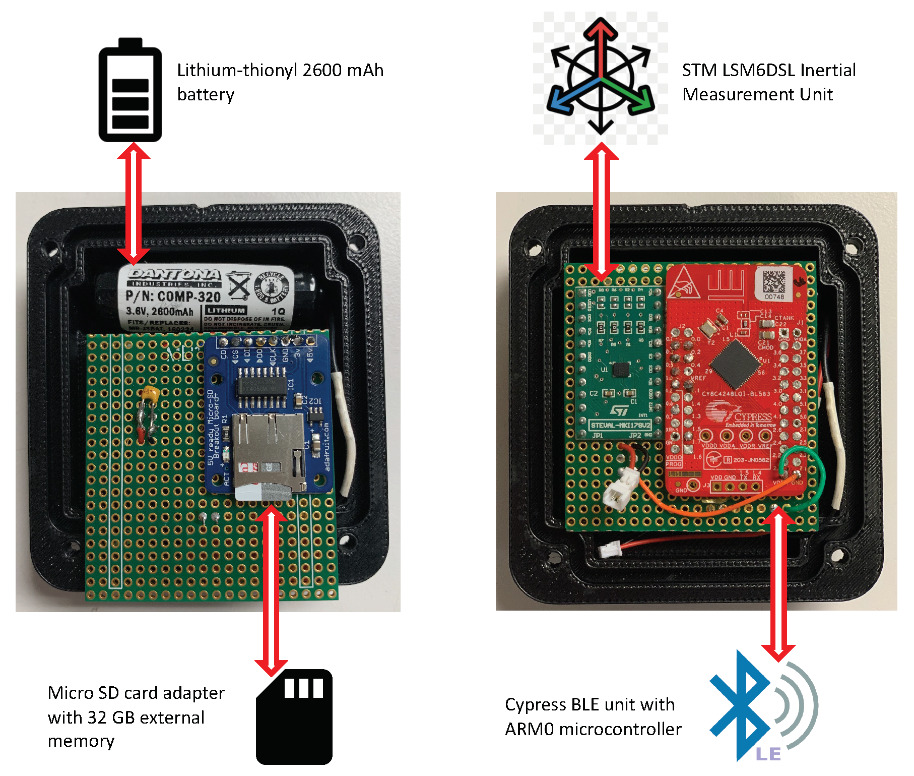
The BLE antenna, in the CY8C4248LQI-BL583 BLE module, consumes 15.6 mA at 0 dBm when transmitting and 18.7 mA when receiving. The processor consumes 1.7 mA at 3 MHz when it is inactive and 1.5 μA when in deep sleep mode [
51]. However, some facts are obscured here. Running the processor at 3 MHz is not valid for our wildlife tracker since some of the external components added to the wildlife tracker depend on much higher frequency clocks; thus, testing at frequencies below 10 MHz is unrealistic for our implementation. The data sheet lists the current consumption at varying CPU clock frequencies; however, it does not include the additional current consumption when BLE communication is active. Thus we had to set a test bench to measure the average current drawn at different clock frequencies while transmitting and receiving advertisement data from the BLE system. This test setup is described and illustrated in the next section.
4.2. Base Case Software Algorithm
The base case algorithm, shown in Algorithm 1, is the initial software algorithm that the wireless sensor nodes ran. The CPU clock is kept at a high frequency of 46 MHz and the transmission power of the BLE device is set to positive 3 dBm. Duty cycling a system to on and off states is proven to increase the power efficiency of that system [
52]. The BLE subsystem in the CY8C4248LQI-BL583 module is set to broadcast and receive every ten seconds for a second. When the BLE subsystem is broadcasting, it transmits an advertisement packet of 31 bytes which holds its name and node ID (Address), and it can also be any custom data. Our current implementation uses the node name and node ID only. During the time in which a node is transmitting it also receives the node names and node IDs of other nodes in the network. It is also important to note that the BLE subsystem, along with the CPU, remained idle yet active, or on, during the period wherein there was no BLE advertising communication.
The flow diagram illustrated in
Figure 3 is a visual of the base case system. First, the system and subsystems, such as the BLE subsystem, are initialized. Then, the program consistently checks if ten seconds have elapsed. If ten seconds have elapsed, then we set the BLE subsystem to discover other nodes and simultaneously advertise. It is important to note that in the algorithm shown here, a state machine is hidden for simplicity. It is also worth mentioning that the ground team in the wild shared that the chimpanzees in a 24 h day roam the sanctuary for 12 h from 6 a.m. until 6 p.m. As 6 p.m. approaches, the chimpanzees move towards the sleeping area and they remain in that area from 6 p.m. until 6 a.m. of the next day. Therefore, our algorithm includes a state machine that places the BLE subsystem to sleep after a 12 h day period. From 6 p.m. until 6 a.m. the system no longer duty cycles the BLE subsystem from non-discoverable and non-advertising to discoverable and advertising.
4.3. Test Bench Hardware Setup
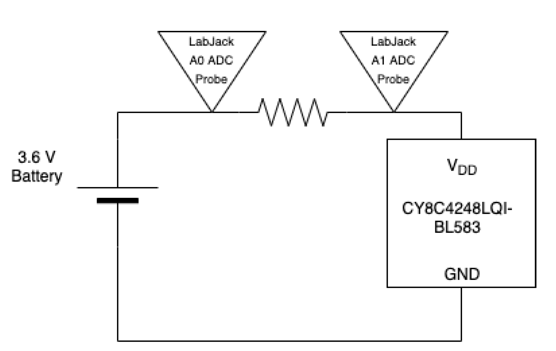
To measure the current consumed by the CY8C4248LQI-BL583 BLE module from the 3.6 volt lithium thionyl chloride battery, we used a 10 Ohm resistor and a measuring device called LabJack T7 Pro. The LabJack T7 Pro can measure voltages through the various analog to digital converters (ADC) at a 12-bit resolution [
53].
Figure 4 shows the configuration of our test setup. To power the BLE module, a 3.6 volt battery with a charge capacity of 2600 mAH is connected in series with it. To measure the current drawn from the device, the power line between the positive terminal of the power supply and the BLE module is broken and the 10 Ohm resistor is placed in between and in series. Two ADCs, A0 and A1 were used to measure the differential voltage of the resistor. This same setup was also used to test our optimized algorithms. Knowing the differential voltage and the resistor value we can calculate the current using Ohm’s Law (
. We then derive the current drawn from the BLE system as:
where
is the current drawn from the BLE system,
is the differential voltage probed by the LabJack T7 Pro instrument, and R is the 10 Ω resistance. Sampling from the LabJack’s ADCs and applying Equation (
3) in software allows us to collect and plot current consumption data. The visuals will later be illustrated. From the derivation of Equation (
3), we can also calculate the instantaneous power consumed by the BLE system by multiplying the voltage of the battery, which is 3.6 V, with the current values obtained in our data.
4.4. Base Case Results
Configuring the base case with the power measurement setup resulted in the data portrayed in
Figure 5. The base case average current when the BLE communication is on is 31 mA. However, when the BLE communication is off and the CPU is left idle, the average current consumed is 17 mA.
Referring to
Figure 6, we can see 1 s pulses with higher current consumption and a lower, 9 s constant current. The high pulses represent a second in which the BLE device is both transmitting and receiving, while the flat current represents 9 s in which the BLE device is idle, neither transmitting nor receiving. From the previous statement, we can conclude that there are two main states for the BLE system; that is, an active BLE state and idle BLE state respectively.
We are also interested in calculating the average current used by the BLE communication system in a 24 h day. It is important to recall that the BLE duty cycling only happens for a 12 h duration in 24 h. In the remaining 12 h period, the BLE communication system is turned off and the CPU is left idle and consumes the average current of 17 mA. However, Equation (
4) is used to calculate the actual average current of the system throughout 24 h.
where
is the average current,
n is the number of different device states,
is the average current in state i, and
is the time spent in state i. The average current for 24 h was calculated to be 17.7 mA. Therefore, multiplying the voltage of the battery, 3.6 V, with the average current, amounts to the average power consumed by the BLE system of 63.7 mW. Given the battery capacity of 2600 mAH and the average daily current, we can also calculate the life span of the system by using Equation (
5).
where
is the battery life in hours,
is the battery capacity in mAh, and
is the average current. Using Equation (
5), we calculate that the system will operate for 146.9 h, which is 6.12 days. In the next sections, we explore different methods to optimize our limited battery capacity and analyze these methods and the improvements they have on power.
4.5. Understanding System Modes
Referring to the CY8C4248LQI-BL583 datasheet, the BLE communication system is a subsystem of the entire BLE module [
54]. The BLE has its own 24 MHz external crystal oscillator (ECO). This ECO is used to generate the correct BLE communication frequency, which is 2.4 GHz. Thus, the BLE is the only peripheral that uses the ECO. When the ECO is in use, more power is consumed; however, as mentioned before, the BLE communication is only established every ten seconds for one second, and this is for both transmission and reception. This means that at all other times, that is, for a 9 s interval, we can place the BLE in one of two sleep modes: sleep mode or deep sleep mode. When the BLE is not being used, in an idle state, the BLE subsystem can be set to sleep mode; however, the ECO is still left on. The ECO can be left on for applications that use the ECO as an external oscillator, or as an input to another subsystem. The system does not make use of the ECO except for BLE communication, and the system’s power can be optimized by placing the BLE subsystem in deep sleep mode. To reiterate, in the deep sleep mode, the ECO is turned off and less power is consumed.
The BLE subsystem also has an internal main oscillator (IMO) for the CPU, which can be set from 3 MHz to 46 MHz with the use of an internal divider. The IMO is used for code instructions, for CPU I/Os, and peripherals that the CPU manages. Similar to placing the BLE subsystem to sleep and stopping the ECO, the CPU oscillator can be put into different modes, including sleep mode and deep sleep mode. Using CPU power mode information from the device data sheet [
55], we can derive:
where
is the current drawn by the BLE module,
is the BLE module CPU frequency, and 17.2 mA is the BLE transceiver average current estimate. Using Equation (
6) we can calculate the theoretical current drawn from the BLE device and can apply this equation to three different frequencies: 14 MHz, 24 MHz, and 46 MHz. The purpose of this calculation is to compare the actual recorded results from the BLE module and validate the small scale test bench. Additionally, the three different frequencies were selected to compare the current and power savings between them.
Table 2 shows the different theoretical currents and actual currents drawn from the BLE device at the different frequencies we are transmitting and receiving.
The percent difference or error to each of these is a product of estimating our average BLE current to be 17.2 mA from averaging the BLE transmission current, 15.6 mA, and the BLE receiver current, 18.7 mA. The averaging assumes that the transmission and the reception use the same amount of time, which is not the case, since the BLE device can be scanning or receiving for a different time interval than the transmission. Explaining the workings of this scheme is not the focus here; however, the rough estimate allows us to determine the validity of our hardware measurement. We obtained less than 10% difference on our hardware validation and we can confidently say that our hardware test bench was measuring accurately.
4.6. Optimizing System Power
Gathering all the information learned, we modified the base case firmware. The flow diagram illustrated by
Figure 7 shows the flow of the updated system. The system components, which are the CPU, the real-time clock (RTC), and the BLE subsystem, are initialized. We then enter a loop and check if 10 s have elapsed. If ten seconds have elapsed, we turn on the BLE subsystem by setting it to discovery mode, which enables reception, and advertisement mode, which enables transmissions. The BLE subsystem can then receive and transmit for a one-second interval. Next, a BLE process event is checked. The system searches if there is any reception or transmission packet that needs to be fulfilled from the BLE stack. If there is, the BLE subsystem architecture takes care of it in the background. However, if the BLE subsystem has no other pending events, such as advertising, attempting to form a BLE connection, or receiving, then it enters the deep sleep mode. The only events that take place in the BLE stack for the system are advertising and receiving during the one-second interval.
The final step to the flow of the software algorithm is to check whether the CPU can be placed in a deep sleep mode as well. The CPU can only enter deep sleep when the BLE subsystem is in deep sleep mode. This criterion is set to ensure that no BLE events are missed. If this condition is met, the CPU system enters the deep sleep mode by turning the CPU IMO off. Additionally, a built-in real-time clock (RTC) is managed via an interrupt that is triggered every second by the watch crystal oscillator (WCO), a low-frequency clock of 32 kHz. Using the WCO is promising in contrast to the IMO or the ECO. The WCO is still accessible when both the BLE subsystem and the CPU are in deep sleep low power modes.
4.7. Optimized Algorithm Hardware Results
We implemented the algorithm outlined in the flow by
Figure 7 on three different frequencies: 14 MHz, 24 MHz, and 46 MHz. Using the same test bench setup with the LabJack T7 pro, we measured both the current drawn when the BLE device is transmitting and receiving and the current drawn when the BLE device is set to deep sleep. Inclusively, we took measurements of the BLE transmission at both 3 dBm and 0 dBm. We noticed that there was no major difference with the amount of current consumed at different BLE transmission powers.
Table 3 shows the currents measured for all frequencies at different transmission power levels and for three different tests.
There is no significant difference between the 0 dBm and 3 dBm settings. Testing for actual average current values for deep sleep resulted in 2 μA for all modules set at different frequencies and different transmission powers. Running the system at 2 μA when the BLE is not in use leads to a significant improvement in power consumption.
Figure 8a–c shows the current consumption during the active portion of the BLE system. The displayed current is specifically taken from our hardware test bench with CPU frequency set at 14 MHz, 24 MHz, and 46 MHz respectively. The transmission power for these configurations was set to 0 dBm. We do not intend to show the current for the 3 dBm configuration as the results are similar. These images are significant, and, in comparison to the base case, when the BLE is idle, we can see that the average idle current dropped to a very small current. The next section will demonstrate that placing the BLE subsystem and CPU into deep sleep has a great and positive impact on power consumption.
Using Equation (
4), we calculated the average current and power for our updated algorithm and the different CPU frequencies in 24 h. The results reflect 12 h of duty cycling the BLE communication to on and off, and a 12 h period where the system is idle. With the updated software algorithm, when the system is in an idle state, the BLE subsystem and the CPU are in deep sleep mode. Placing the idle states in deep sleep allows us to significantly increase the power performance of the system, since the idle current is then 2 μA instead of 17 mA.
Table 4 shows the power performance improvement between the different CPU clock frequencies and the base case configuration. The percentages of improvement at the different CPU frequency configurations are comparisons of improvement in power performance against the base case algorithm at a frequency of 46 MHz.
Table 5 shows the comparison and improvement in battery life against the base case algorithm. The comparison is shown in both hours and days. At 14 MHz the battery lives well over six times longer, at 24 MHz the battery lives well over five times longer, and at 46 MHz, which is the same frequency as the base case algorithm, the battery lives over five times longer as well.
5. Scaling Up Power Optimization Using a Dynamic Wireless Node Simulator
In this chapter we further explore the power saving values of our method by varying the active triggering time interval of the BLE communication. The wireless sensor node was deployed to advertise and receive for one second for every ten seconds; however, we want to see greater improvements in power consumption. We want to analyze the power savings for active triggering time intervals greater than ten seconds. This suggests that the BLE communication will be less active which would lead to less power consumption. To verify this on a large scale, we developed a simulator that uses our actual current hardware results listed in the previous chapter. The simulator uses Equation (
4) to calculate the current and derive the average power and the lifetime of a wireless sensor node with varying BLE active triggering intervals. We know that increasing the BLE active triggering interval will affect the throughput of the network. For our purposes, the throughput is the total number of nodes that can be read within the vicinity of a particular node that is set by a threshold. In a later section, we mention that that the threshold is a 10 m radius. The simulator will also verify the impact power optimization, through larger BLE active triggering intervals, has on the throughput of the network. We are interested in continuing to optimize the power performance of the wireless sensor nodes; however, we do not want to compromise the QoS of the network. In summary, the simulator will verify the increased power performance for varying BLE active triggering intervals and it will verify the impact it has on the network’s throughput performance. It is important to address that without the simulator, verifying the trade-off between power and the network throughput performance would require extensive testing, observations, and analysis. Our goals with simulations are as follows:
Make feasible experiments for various unique network settings, scaling the network size up.
Analyze the optimization of power by setting different lengths of active triggering time intervals.
Ensure that further power optimization does not degrade network throughput.
5.1. Simulator Overview
Though the simulator allows us to explore improvements to our algorithm’s power performance, it is of significant importance that it can mimic realistic random movements of wireless nodes. Specifically, the wireless nodes represent the movement of chimpanzees in a sanctuary. For our purposes and simplicity, we condense the sanctuary to be represented by 1 hectare, an area of 100 m by 100 m or 10,000 square meters. We also know the following information:
The chimpanzees have a designated area for feeding.
The chimpanzees are free to move in this area throughout 12 h in a day.
The chimpanzees have a designated time to sleep and have a designated area to sleep.
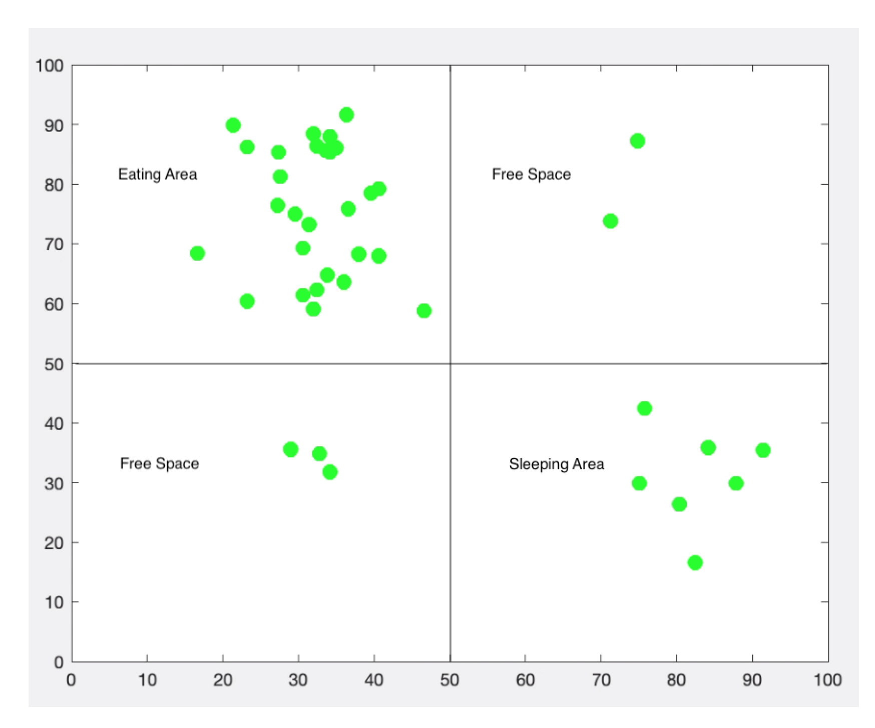
We divided the hectare area into four quadrants. From left to right and top to bottom, the first quadrant represents the feeding area, the second and third quadrants represent areas in which the chimpanzees are free to roam around, and the fourth quadrant represents the designated sleep area.
Figure 9 gives a visual of the quadrant assignments. The visual shows the wireless sensor nodes, which would be placed on the chimpanzees as green dots; however, each chimpanzee is represented by a specific and unique coordinate.
The simulation runs for a specified time in seconds. The chimpanzees will move to different quadrants at given times throughout the day. For example, at around noon, the chimpanzees are fed in a designated area and at a specified time. The chimpanzees know this and will begin to move to that area once the time approaches. Analyzing
Figure 9, we can tell that the feeding time was near, as most of the chimpanzees (nodes in green) were in quadrant I, the eating area. Similarly to this example, other events take place based on the chimpanzees’ behavior. Recall that the wireless sensor nodes capture the interactions an individual animal has with another animal based on their proximity. We want the simulator to capture data as the wireless sensor nodes would in a real-world scenario.
5.2. Simulator Model
For the simulator to behave as realistically as the chimpanzees moving through the sanctuary, we used Markov chains. A Markov chain is a stochastic process where the next state of a system only depends on the present state [
56]. The Markov chain state diagram we implemented is shown in
Figure 10, where each circle represents a state of a chimpanzee in a given quadrant. The first quadrant is the eating area, the second and third quadrants are free space area, and the fourth quadrant is the sleeping area. The diagram also includes directional arrows from one state to another, including a directional arrow from a state to itself. Each directional arrow contains a weight which is the probability from transitioning from the present state to the next state. Mathematically, the probability from one state to another can be represented and shown in Equation (
7) [
57]. This equation represents the conditional probability a chimpanzee transitions from one region
i at time
t to another region
j at time
. The conditional probability is then represented as
, and is shown in
Figure 10 near each state transition or directional arrow. We use half an hour or 1800 simulated seconds as the granularity of time
t.
We mathematically translate the Markov chain and use a matrix called the transition matrix, or probability matrix, to model the transition from one state to another. A transition matrix contains the probabilities for each state transition shown in
Figure 10. The transition matrix contains rows and columns that represent each state in the Markov chain. Specifically, the rows represent the current state at a given time
t. The columns represent the next state of a transition that will take place at time
. Thus, each element in the transition matrix contains the conditional probability of transitioning to the next state
j given the current state
i, where
and
.
It is important to address that a single transition matrix represents a single event in the simulation. This happens because different events occur throughout a chimpanzee’s day. An event can be classified as a process that drives a chimpanzee to a specific response. For example, when a chimpanzee knows that the feeding time approaches, the chimpanzee will move towards the eating area with a higher probability. Thus, different time boundaries trigger different events, or Markov chains, in which different probabilities are used to determine the transition of a chimpanzee from one area to another. To account for important events, we created a transition matrix for different activity movements observed from the chimpanzees. We have a total of five probability matrixes which represent the following activities: uniform movement throughout the four quadrants, movement towards the designated eating area, active movement after the chimpanzees are fed, movement towards the designated sleep area, and still movement, which represents grooming. The probability matrices are in Equation (9).
Each row and column pair represents a state transition. The left-most column and the rightmost column represent quadrant 1 and quadrant 4 respectively. Similarly, the topmost and the bottom-most rows represent quadrant 1 and quadrant 4 respectively. The rows represent the current quadrant and the columns represent the quadrant a chimpanzee is transitioning into. Thus, the index pair (row = 1, column = 2) represents the state transition from quadrant 1 to quadrant 2. If the column were to be column equal to 3, then that index pair would represent state transition from quadrant 1 to quadrant 3, and so on for the remaining index pairs. Therefore, a transition matrix is used to represent the transition of a chimpanzee when it is found in a quadrant at a particular time. For example, the uniform matrix has an evenly distributed probability of 25% for each of the quadrants. This suggests that a chimpanzee has equal probability to transition to any of the four quadrants or areas, including its current quadrant position. The active matrix suggests that a chimpanzee is most likely to move to other quadrants, with equal probability, but with a lesser probability to stay in the quadrant that the chimpanzee is currently in. Thus, for the current quadrant, there is only 10% probability and the remaining probability is evenly spread amongst the other quadrants—that is, 30% each. The sleep matrix is used to represent the times of day where the chimpanzees are most likely to be in or near the sleeping area. Thus, the matrix holds a much higher probability in column 4, which represents that there is a higher probability for a chimpanzee to transition towards the sleeping area. The eat matrix is used to model the movement of the chimpanzees during their time to feed. Thus, a higher probability is assigned in column 1. The other quadrants were assigned much smaller probabilities but evenly distributed. The still matrix models the times that a chimpanzee is most likely to stay in its current area. Thus, the diagonals hold the highest probability and the other entries hold much smaller, but evenly distributed, probabilities. The simulator is not limited to these transition matrices, but versatile enough to work with additional transition matrices if needed.
The transition from one state to another state also depends on time boundaries that signal a different Markov chain. It is at the time boundaries a simulated chimpanzee, with a wireless sensor node, is able to transition from one area to another. These time boundaries are simulated time events that occur in a real world scenario. The time boundaries are as follows:
: The start of the day, which is second 0 of the day.
: The time the chimpanzees begin to move away from the sleeping area.
: The time at which the chimpanzees begin to be feed and go to the feed area.
: The time at which the chimpanzees are no longer fed.
: The time at which the chimpanzees begin to move to the sleep area.
: The time interval at which the currently selected probability matrix should set the new position of the nodes in the wireless full mesh network.
5.3. Simulator Algorithms
The simulator needs an algorithm that can feasibly perform our goals. The flow diagram of the algorithm is depicted in
Figure 11. The simulator’s algorithm is outlined in Algorithm 1, and it implements the Markov chain model. It also uses the hardware calculations obtained from
Section 4 and contains several parameters that must be predefined.
The simulation framework is implemented with MatLab [
58]. The algorithm has four main loops. The first loop iterates through the different number of nodes in the node list.
n, the current number of nodes, defines the density of the wireless full mesh network for the current iteration. The second loop iterates through the different active period intervals and sets the active period interval,
, for each of the nodes,
n, in the current iteration. The third loop iterates through 50 random seeds for the current wireless full mesh network that consists of the current number of nodes,
n, and the current active interval period,
. Once we are in the inner loop, we take the current seed,
s, and set the random seed generator on that seed. We then initialize the position of all the nodes into the defined grid of 100 m by 100 m. The fourth loop represents the time, in seconds, the BLE system is in use. It particularly represents the 12 h period, from 6 a.m. to 6 p.m., that the node is switching between its active cycle and sleep cycle. During the latter 12 h of a day, from 6 p.m. to 6 a.m., the wireless sensor node is placed in a deep sleep state; therefore, there are no throughput data, and the average current consumption of a wireless sensor node during this period is constantly at 2 μA. Inside the timing loop, we set the new position for each network node. The new position is calculated using Algorithm 2. Let us analyze Algorithm 2 in depth.
| Algorithm 1: BLE dynamic node simulator for a full mesh network |
Required: Deployed area in meters, Area Divided into Quadrants, Probability Matrices, Time Boundaries, Define WSN Distance of Rx Sensitivity, List for Different number of Nodes, Set Distance of Rx Sensitivity, List for Different BLE active period intervals, Number of Random Seeds
- 1:
for n = node in [10, 15, 20, 30, 40, 50] do - 2:
for ble_active_triggering_interval=bleactivetriggeringintervalin [10, 12, 15, 20, 25, 30, 35, 40, 45, 50] do - 3:
for s = seed in [1...50] do - 4:
setRandomSeed(s) - 5:
positionOfNodes = createNetworkMatrix(n) - 6:
for t = time in [1...(12 × 60 × 60)] do - 7:
positionOfNodes = getNewPositionofNodes() - 8:
if then - 9:
probability_matrix=uniform_probability_matrix - 10:
else if then - 11:
probability_matrix = eat_probability_matrix - 12:
else if then - 13:
probability_matrix = active_probability_matrix - 14:
else if then - 15:
probability_matrix = sleep_probability_matrix - 16:
else - 17:
probability_matrix = still_probability_matrix - 18:
end if - 19:
if then - 20:
positionOfNodes = moveQuadrant(probability_matrix) - 21:
end if - 22:
if then - 23:
throughput_matrix = recordThroughput(positionOfNodes) - 24:
end if - 25:
end for - 26:
recordThroughputPerNodeAtCurrentRandomSeed() - 27:
end for - 28:
recordAverageThroughputPerNodePerActivePeriodInterval() - 29:
recordStandardDeviationOfThroughputPerNodePerActivePeriodInterval() - 30:
calculate24HourPowerConsumptionPerActivePeriodInterval() - 31:
end for - 32:
recordNetworkAverageTotalThroughput() - 33:
end for
|
| Algorithm 2: Calculate the new position of a node in the full mesh network |
Require: Current X and Y coordinates, Step Size Gain
new_position_x_max = current_position_x + step_size new_position_x_min = current_position_x - step_size new_position_y_max = current_position_y + step_size new_position_y_min = current_position_y - step_size new_position_x = randChoose(new_position_x_max, new_position_x_min) new_position_y = randChoose(new_position_y_max, new_position_y_min)
|
To calculate the new position of a node, we need the current node position in both coordinates and the step size at which the node can change for both coordinates. We set the nodes to move by a step of 0.1 m, which is set as a constant during the simulation. With these parameters, the algorithm finds the new maximum position and minimum position for both the X and Y coordinates by adding the step size and subtracting the step size respectively from both the X and Y coordinates, obtaining the minimum and maximum coordinate values after a movement in one time step. The last step is to randomly choose a position within the movement range for both coordinates. Back to Algorithm 1, the next step is to check the time boundaries to set the appropriate transition matrix. Setting the correct transition matrix is crucial so that the simulation can closely track a real-world scenario. If we are within the time interval , we set the new positions of the wireless nodes based on the transition matrix. As mentioned before, the transition matrix determines the new quadrant and position of each node stochastically. Algorithm 3 shows the algorithmic process to determine a node’s new quadrant and position when a transition matrix is activated.
| Algorithm 3: Move node position utilizing the probability matrix |
Require: Current 4 × 4 Probability Matrix, X and Y Coordinate of each node
current_quadrant = determineCurrentQuadrant(X, Y) cumulative_probability_array = computeCummulativeProbabilityArray(current_quadrant, curren_probability_matrix) random_probability = getRandomProbability() for single_cumulative_probability = cumulativeprobabilitiesin cumulative_probability_array do if then if ) then next_quadrant = quadrant break end if else if then next_quadrant = single_cumulative_probability_index break end if end if end for
|
Algorithm 3 begins with the given X and Y coordinates of the node to determine the current quadrant in which the node is located. Next, we calculate the cumulative probability array using individual probability values in respective transition matrix. These probabilities each represent a probability at which a node in the current quadrant can transition to any of the four quadrants. Returning to Algorithm 3, a random probability is generated and assigned to a variable called . The algorithm iterates through the different cumulative probabilities in the array . If the random probability, , lies within the boundaries of two cumulative probabilities in the cumulative probability array, then the next quadrant is equivalent to the index of the current iteration. The index is given the variable name .
Back to Algorithm 1, the last step in the inner loop is to verify that the current "time" corresponds to a time at which the BLE should be actively transmitting and receiving—this simulates the wireless sensor nodes’ behavior, which is determined by the software algorithm. If it does, then we record the throughput based on the current positions of the nodes and store that information in a matrix called . The next lines to the algorithm simply record all the valuable information that we need to analyze power and throughput performance for the different combinations of network densities, different BLE active triggering intervals, and different initial node locations.
5.4. Simulator Parameters
Our wireless sensor node is meant to detect proximity with respect to other nodes. Field researchers placed the constraint of ten meters and below on meaningful proximity data. In the simulator, there is node-to-node throughput or communication when the Rx (reception) sensitivity is an equivalent distance of 10 m or less. As mentioned in
Section 4, we use the actual hardware results pertaining to the current drawn from our experiments in
Section 3 to find the correct hardware parameters. We took different current measurements of the BLE system at different CPU clocks or frequencies. The simulator takes a list of the hardware’s actual average currents with respect to the BLE transmission at different CPU clocks. Therefore, the simulator will loop for each CPU frequency and record data for the BLE system set at that particular clock. The list consists of the following currents for 14 MHz, 24 MHz, and 46 MHz respectively: 19.5 mA, 23.3 mA, and 27.7 mA.
A major goal for the simulations is to scale up and test several network densities; therefore, we specify a list of the different numbers of nodes for a full mesh network. The node list consists of: 10 nodes, 15 nodes, 20 nodes, 30 nodes, 40 nodes, and 50 nodes. Node counts of 10 nodes, 15 nodes, and 20 nodes are more realistic and align more with the number of nodes that cognitive science researchers would want to initially deploy. However, we wanted to show that the system could work for a larger wireless full mesh network. Additionally, we would like to see the power and throughput results with the wireless sensor nodes with different BLE active triggering intervals. To analyze the impact of the distinct BLE active triggering intervals, we use the following times: 10 s, 12 s, 15 s, 20 s, 25 s, 30 s, 35 s, 40 s, 45 s, and 50 s. Note that the first three intervals differ by 2 s and 3 s respectively. This was done to analyze the effect between smaller increments in BLE active triggering time intervals. We gathered data that showed an improvement in the power performance, with drop in throughput, however. With power and throughput data we can discover the optimal solution for the wireless sensor node.
To model animal movement, we use Markov chains that consist of transitions from one area to another. For example, we specifically know that the chimpanzees start and end their day in a designated area for sleeping. We also understand that they can move differently each day or start and end their day differently. At the beginning of a day, an individual may start at a different coordinate or location. Thus, we gather network throughput data for different days, by running experiments with fifty random seeds for each node number and BLE active triggering interval pair. A summary of the important simulator parameters is listed in
Table 6.
5.5. Results
After running our algorithm for various scenarios, we gathered information regarding power consumption and corresponding throughput values. Many scenarios will not be covered, but the most crucial data will be analyzed and discussed.
5.5.1. Power Results
The power results depend on the BLE active triggering interval and the CPU frequency of the wireless sensor node. The wireless sensor node is duty cycling between an active BLE communication and no BLE communication for 12 h. Activating the BLE communication depends on the BLE active triggering interval, . This means that every seconds the BLE communication is on for a one-second interval. In the remaining 12 h, the wireless sensor nodes are in sleep mode and only consume 2 μA. For different CPU frequencies, the simulator sets the nodes to simulate current consumption based on one of the following three currents: 19.5 mA, 23.3 mA, and 27.7 mA. The currents correspond to the CPU set at 14 MHz, 24 MHz, and 46 MHz respectively. We obtain information for the nodes with different combinations of BLE active triggering intervals and CPU frequency currents. For each combination, we obtain different power results. Since we have three different current consumption values, based on the three CPU frequencies, and 10 different BLE active triggering intervals, we obtain 30 power results. All power results (average current, average power, node lifetime) apply to a single node.
As we increase the BLE active triggering interval, the average power consumption drops. This is true at all frequency settings, however, recalling from the hardware experiments, the current drawn from the BLE device at a higher frequency is higher. Thus, at higher frequencies, we experience higher power consumption in comparison to lower frequencies. To compute the average power, we first use Equation (
4) to obtain the average current consumption in a simulated 24 h day. This current is then multiplied with the voltage of the battery, which is 3.6 V. The results are shown in
Table 7 and represent the average power consumed for a single wireless sensor node in 24 h.
Next, we calculate the percentage of average power saved between adjacent values in the list of BLE active triggering intervals. That is, the average percentage of power saved between 10 s and 12 s, 12 s and 15 s, 15 s and 20 s, etc. The percent of power saved transitioning from one frequency to the other shares a similar pattern.
Table 8 shows the percentages calculated. By thoroughly examining the numbers, we can see that the power saving increases when transitioning from 10 s to 12 s, 12 s to 15 s, and 15 s to 20 s. As we transition from a large BLE active triggering interval to a slightly larger active triggering interval, our power saving begins to decrease significantly. As the BLE active triggering interval grows larger, the system as a whole consumes much less power since the system duty cycle is kept longer in deep sleep. Thus, approaching larger BLE active triggering intervals we approach closer to a more constant deep sleep average power.
Figure 12a is a visualization of the power saving pattern across all three frequencies. As seen in the plot, the peak saving is made between the transition of 15 s to the choice of a 20 s BLE active period interval.
We explore further power savings by increasing the BLE transceiver active triggering interval. The results are shown in
Figure 12b,c. A larger BLE active triggering interval is inversely proportional to the current consumed by the system. When the BLE communication is less frequently active there are current savings that will correlate to power savings. Thus, the lifetime to the wireless sensor node is directly proportional to the BLE active triggering interval and we see the lifetime increase. The percent power improvement from the base case ranges from 92.16%, which sets the CPU at 46 MHz and the BLE active triggering interval to 10 s, to 98.89%, which sets the CPU at 14 MHz and the BLE active triggering interval to 50 s. The lifetime of a node ranges from 78.11 days to 549.97 days for the respective settings. This is a significant improvement from the base case lifetime of 6.12 days.
5.5.2. Throughput Results
As shown in
Table 6, throughput is the number of times a node reads another node in its vicinity, and it is not limited to reading one node but can read multiple nodes. The average throughput for a single node is the average throughput for fifty distinct n-dense network events, where
n is the number of nodes in a network event. An event is composed of multiple unique interactions that each node has with other nodes during the time that the network is active. The total average throughput of the network is the sum of all the nodes’ average throughputs. The throughput results depend on the network density. The more nodes there are, the more probable that a single node can record more neighbors. The throughput results also depend on the number of events, which in our case is set by fifty random seeds and fed to a random generator. The last parameter is the BLE active triggering interval because this parameter turns on the BLE communication for one second every
ble_active_triggering_interval number of seconds. Therefore, the longer the BLE active triggering interval is, the fewer times the BLE communication broadcasts and receives. This affects two aspects of the network. First, a longer BLE active triggering interval suggests that a node makes itself known less to other nodes. Second, a longer BLE active triggering interval suggests that a node can read other nodes in its vicinity less frequently.
Throughput changes are significant between the different combinations of node count and BLE active triggering intervals. The throughput results are important, as they allow us to understand the impact our power-saving algorithm has on the performance of our full mesh network.
Figure 13a shows the average total throughput data with different network densities and different active period intervals. Looking at this figure, we see the average throughput decreases as active triggering interval gets bigger. We show that increasing the BLE active triggering interval decreases the power consumption at the expense of the network’s performance.
Next, we show the throughput percent drop as the ratio of the throughput of any of the BLE active triggering interval that is greater than ten seconds over the throughput for the base case (10 s).
Figure 13b depicts the throughput decrease with increasing BLE active triggering interval. We see that the throughput decrease is larger for longer BLE active triggering intervals. Note that the throughput decrease is similar for different network sizes; thus, we show only one line in this figure. For our particular application, we do not want to lose more than 50% throughput, in order to obtain consistent and meaningful tracking data. If we desired to further optimize the power consumption of the system, BLE active triggering intervals below 20 s are the better performers for our purposes.
5.5.3. Scaling Up the Network Size
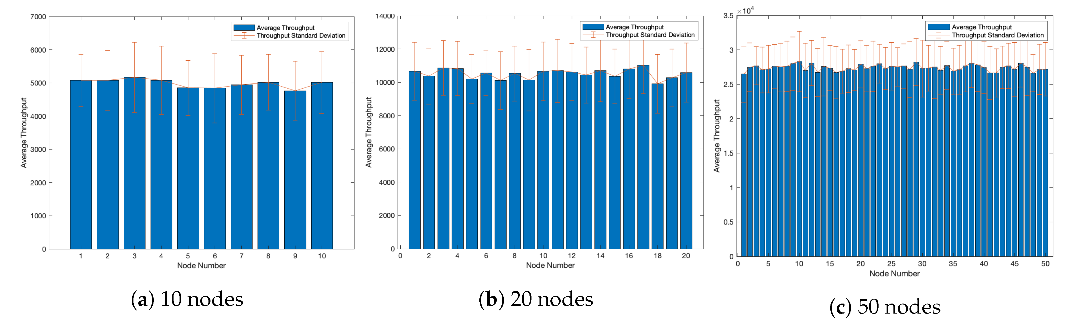
This section analyzes the effect of scaling up the network size. To do this, we analyze each node’s average total throughput and the standard deviation between the total average throughput for fifty random events. The average throughput for each node along with its respective standard deviation can tell us the variability that would be expected if the experiment would be repeated.
Figure 14a shows the average total throughput for ten nodes for a simulation event in the thick blue bars. It also contains an error line which represents the standard deviation per average bar. This percentage in the error bar tells us the uncertainty in our reported throughput measurement. Let us examine a network with twice as many wireless nodes. Referring to
Figure 14b, we see that the maximum variation happens at node number 11. The percent difference the node experiences from the average throughput is 17.72%, which is less than the previous example.
Figure 14c shows the error bar for our densest network of 50 nodes. Node 32 experiences the highest variation in its average throughput for 50 random events, and the percent difference from the average throughput is 16.53%.
We took a further step and expanded our tests to include a network with size 75 and 100. The average throughput per node in 50 random events was generated for these network densities. Since we are interested in the variation and uncertainty, we plotted the maximum coefficient of variation per n-dense network. The coefficient of variation consists of the throughput standard deviation between a node’s recorded throughput in 50 random events, divided by the average throughput for that same node in those same events. We take the maximum coefficient of variation since this indicates the largest variation we see per n-dense network. The coefficient of variation in the simulator, for network densities ranging from 10 nodes to 100 nodes, is illustrated in
Figure 15. The results show more throughput variability for less dense networks relative to the average throughput per node. Hence, there is more confidence in denser networks. As the network size scales up, the simulator can handle it with diminishing variation.
6. Conclusions
This paper evaluated the design of an energy-efficient network used for wildlife observation. The network consists of a full mesh topology and contains nodes that communicate via Bluetooth Low Energy (BLE) in advertisement mode. The initial hardware configuration and software algorithm duty cycles the BLE communication to on and off states using a parameter called the BLE active triggering interval. This parameter triggers the BLE communication to be on for 1 s. Turning the BLE communication to off results in lower power consumption. The base case wireless sensor node has a BLE active triggering interval of 10 s and a CPU clock set to 46 MHz.
The algorithm was improved by placing the BLE subsystem and CPU in deep sleep when there are no BLE or CPU tasks to process. This alone improves the power performance by 92.16%. We improve power performance further by 93.41% and 94.48% by changing the CPU clock of the wireless sensor node from 46 MHz to 24 MHz and 14 MHz, respectively. To further optimize the power of our device, we used longer lengths of BLE active triggering intervals. This implies a drop in the network’s throughput performance. We tracked this effect for varying network densities by scaling up power optimization and analyzing the trade-off between power and throughput. We created a simulator that models our network with dynamic wireless sensor nodes. The simulator verified the base case hardware results. It also showed a median power performance increase of 97.79% in comparison to the base case, yet a throughput decrease of 66.65%. The highest power performance increased by 98.89% when a wireless sensor node was configured with a BLE active triggering interval of 50 s and its CPU was set at 14 MHz; however, the simulator showed the throughput drop by 79.97%. Depending on the application, a design may tolerate the decline in throughput to achieve higher power performance.


