Experimental Performance Analysis of an Optical Communication Channel over Maritime Environment

Abstract

Free space optical communications (FSO), which make use of the visible and infrared spectrum for data transmission, offer significant advantages such as a very high data rate, security and immunity, low cost of installation and ease of use without any license restrictions. However, a significant challenge for FSO systems is their inherent constraints due to environmental conditions and especially atmospheric turbulence. This paper focuses on the experimental performance analysis of a real FSO system in a maritime environment. We propose a new model which allows an FSO link performance estimation over sea and depends upon point measurements of environmental parameters. The Received Signal Strength Indicator (RSSI) has been measured and a second-order polynomial has been constructed using regression modeling to quantify its relation with macroscopic environmental parameters collected by a weather station. This model has then been validated against real meteorological data over different period of times and exhibited a reasonably strong correlation. Atmospheric turbulence has been determined using bulk estimates of the structure index parameter extracted from the same meteorological data, and thus allowed for a statistical correlation between turbulence and RSSI. In the second part of the paper, the probability distribution of the RSSI data has been investigated and the Kullback-Leibler (KL) divergence has been used to investigate the difference between probability distributions over the same variable. As an illustrative example of the process, the Weibull, Lognormal and Gamma distributions have been evaluated against the RSSI data probability distribution and the latter has proved to exhibit the best fit.

1. Introduction

Free space optical (FSO) communications is a significant application of the laser technology initially developed in 1960 [1]. Since then, much research has been conducted into FSO communications and different applications have been demonstrated, including terrestrial, maritime, space and deep space applications [2]. Despite the initial uncertainties about its potential, the ongoing development of optoelectronic devices and its proven success in military applications provided the required boost to continue investments in the field [2]. FSO technology offers significant advantages over its RF counterpart and benefits applications in platforms with increased weight and space limitations [3]. The principle advantages of FSO communications include increased bandwidth, greater security and immunity, lower cost of installation and, finally, no license restrictions [2]. However, FSO communications are susceptible to various atmospheric effects and phenomena, including molecular and aerosol absorption and scattering as well as atmospheric turbulence. The performance of a laser communication link is highly affected by these phenomena that can ultimately cause temporary link interruption [4]. The evaluation of the impact of these effects on the performance of a real laser communications link over maritime environment is the primary objective of this paper. To the best of the authors’ knowledge, it is the first time the performance of a real FSO link over maritime environment is evaluated using accurate local meteorological parameters.

Atmospheric turbulence can be a major degradation factor for an FSO link and, therefore, extensive theoretical and experimental research work has been devoted to quantify its effects on atmospheric laser propagation. For example, the Naval Research Laboratory have been operating a laser communications test facility where a 32-km retro-reflected link has been demonstrated at data rates up to 2.5 Gbps [5,6]. Along with these measurements, atmospheric characterization of the optical path over the maritime environment has also been investigated. In [7], a novel analogue FM ship-to-shore communications system has been utilized to successfully demonstrate bidirectional video and audio transmission along a 3-km link. In [8], a measurement campaign over a 15-km range has been set up and all propagation effects have been investigated quantitatively. In [9], a very promising experiment took place during a US Navy sea trial exercise where the capabilities of a short ship-to-ship FSO link to transfer data obtained during a maritime interdiction operation have been investigated, proving that laser communication systems can complement their RF counterparts in the near future. In [10,11], the effects of humidity and temperature on the performance of an FSO link operating in a coastal environment have been investigated. In those works, two mathematical models that linked the FSO attenuation coefficient to the humidity and the air temperature or dew point, respectively, have been proposed. In [12], Michael et al. exploited scintillation measurements from a 5-km horizontal path optical link to compile ensemble probability distributions and compare those with standard channel models such as the lognormal and gamma–gamma distributions. In [13,14], the bit rate of a commercial FSO link over maritime environment has been measured under weak to moderate turbulence conditions. The observed data probability distributions have been compared to theoretical Lognormal and Gamma distributions and demonstrated a very good fit. In [15,16], Tunick used optical scintillometer data collected from a near-horizontal path to explain the physical relationships between refractive index structure parameter and microclimate fluctuations. By using regression analysis, it has been shown that there is high correlation in 8 out of 21 cases studied. Still, others have shown a correlation between the RSSI—a metric of the link performance—and local macroscopic meteorological parameters [17,18,19].

The purpose of this paper is to explore the performance of a commercial FSO link in a maritime environment. Since measuring directly an optical link over sea is rather difficult, it is very helpful to construct simple models for optical link performance quantification based upon routinely single point-measured environmental parameters. To this end, a second-order polynomial model is proposed to predict the RSSI of the system based upon local macroscopic parameter measurements. The collected data spanned over a period of approximately 40 days, within which the fluctuations of these parameters were quite intense. The model was validated twice against observed data in later periods and proved to be very accurate, i.e., a correlation >0.8. The model includes basic meteorological parameters, including wind speed, air temperature, humidity, air pressure, solar radiation, dew point, and rainfall rate. By utilizing well known models available in the open technical literature for the refractive index structure parameter, $C_n^2$, we estimated its value for the same periods and correlated these values with the modelled RSSI values. Finally, the probability density function of the RSSI data has been compared against standard channel models, i.e., Gamma, Lognormal, Weibull, and the best fit is estimated using the Kullback-Leibler (KL) divergence. The rest of the paper is organized as follows. Section 2, provides the background of atmospheric turbulence and presents the literature models for $C_n^2$ estimates. Section 3, describes the whole experimental setup, which was located across the entrance of Piraeus port. Section 4, presents and analyzes the findings of the measurements whereas Section 5 concludes the paper.

2. Atmospheric Turbulence

Optical propagation through the atmosphere experiences disturbances due to small spatial and temporal fluctuations of the refractive index. These fluctuations comprise the so-called optical turbulence and range in size from a few mm to a few meters [20]. These random changes of refractive index cause various deleterious effects to the optical wave, including irradiance fluctuations, i.e., scintillation, beam wander and beam spread.

Due to the nonlinear nature of turbulent motion, it is rather difficult to predict the strength of this phenomenon in a specific point around space. Instead, a statistical description is used to characterize the strength of the refractive index variations. For mathematical simplification purposes, the axiom of statistical homogeneity and isotropy is utilized for this statistical description [1]. Small-scale temperature fluctuations lead to the definition of the temperature structure function, D_T(R), as derived from the Kolmogorov theory which follows the two-thirds power law [20]:

$$D_T\left(R\right)=\langle {\left(T_1-T_2\right)}^2\rangle =\{{}_{C_T^2{R}^{2/3},\hspace{0.17em}\hspace{0.17em}{l}_0<R<L_0}^{C_T^2{l}_0^{-4/3}{R}^2,\hspace{0.17em}\hspace{0.17em}0\le R\le l_0}$$

(1)

where T₁ and T₂ are the ambient temperatures at two different points in space, separated by the distance R, l₀ and L₀ the inner and outer scale of turbulence while $C_T^2$ stands for the temperature structure parameter. These temperature fluctuations result in atmospheric index of refraction fluctuations. The refractive index, n(R), assuming that time variations are omitted, can be mathematically evaluated in a point R as [20]:

$$n(R)=1+n_1(R)$$

(2)

where the unity represents the mean value of the index of refraction and n₁its random deviation from the mean value.

These refractive index fluctuations are related to the temperature and pressure fluctuations as [20]:

$$n(R)\cong 1+79\times {10}^{-6}\frac{P(R)}{T(R)}$$

(3)

where P is the atmospheric pressure in millibars and T the local temperature in Kelvin. The strength of these fluctuations are characterized by the refractive index structure parameter, related to temperature structure function as [20]:

$$C_n^2=\left(79\times {10}^{-6}\frac{P}{T^2}\right)C_T^2$$

(4)

From Equations (1) and (4), it can be deduced that simultaneous temperature measurements of two points with a known distance between them allows for the direct calculation of $C_T^2$ and, consequently, $C_n^2$. Assuming that the turbulence is well described by Kolmogorov theory, then $C_n^2$ should (on average) be independent of the separation distance between the two points as long as l₀ < R < L₀. This method to estimate turbulence strength from simple point temperature measurements has been used before, e.g., see [21].

The prediction of $C_n^2$ has been a topic of extensive research. Most of experimental research works have applied different methods to measure $C_n^2$ and validated them by path-averaged scintillometer measurements. However, there exist a few mathematical models that have demonstrated very good fit to observed measurements and are based upon macroscopic meteorological models [22]. Some of the more prominent models in the open technical literature is the Huffnagel-Valley model, the Huffnagel and Stanley model and the Submarine Laser Communications (SLC) Day and SLC night models [22].

On the other hand, Sabot and Kopeika, have also proposed two simple mathematical models to predict $C_n^2$ strength based upon macroscopic meteorological parameters which can be easily obtained from a local weather station [23]. The first model can be mathematically expressed as [23]

$$\begin{array}{ll}{C}_n^2& =3.8\times {10}^{-14}W(t)+2.0\times {10}^{-15}T-2.8\times {10}^{-15}RH+2.9\times {10}^{-17}R{H}^2\\ & -1.1\times {10}^{-19}R{H}^3-2.5\times {10}^{-15}WS+1.2\times {10}^{-15}W{S}^2-8.5\times {10}^{-17}W{S}^3-5.3\times {10}^{-13}\end{array}$$

(5)

where W(t) is a weight function, T is the air temperature in Kelvin, RH the relative humidity in hPa and WS the wind speed in m/s.

The second model, apart from wind speed and relative humidity, takes into account the solar flux in Cal/(cm²·min) and the total cross-sectional area of particles in cm²/m³, namely [23],

$$\begin{array}{ll}{C}_n^2& =5.9\times {10}^{-15}W(t)+1.6\times {10}^{-15}T-3.7\times {10}^{-15}RH+6.7\times {10}^{-17}R{H}^2\\ & -3.9\times {10}^{-19}R{H}^3-3.7\times {10}^{-15}WS+1.3\times {10}^{-15}W{S}^2-8.2\times {10}^{-17}W{S}^3\\ & +2.8\times {10}^{-14}SF-1.8\times {10}^{-14}TCSA+1.4\times {10}^{-14}TCS{A}^2-3.9\times {10}^{-13}\end{array}$$

(6)

Both empirical models are valid under specific limits of the macroscale parameters, i.e.,

9 °C < T < 35 °C

14% < RH < 92%

0 m/s < WS < 10 m/s

0 W/m² < SF < 1000 W/m²

The $C_n^2$ strength is strongly height dependent. The highest values are observed at almost zero altitude, whereas at higher altitude decrease rapidly [24]. The above models have used a height of 15 m, therefore all subsequent users need to scale them in the desired height [21]. A typical diurnal profile of $C_n^2$ is characterized by higher values during the day, with a peak around midday and lower ones during night. The lowest values appear around sunrise and sunset. In order to emphasize this profile, both models include a weight function, calculated on the basis of the temporal hour that relates the actual time to the times of sunrise and sunset [21]:

$$H_T=12\frac{H_{actual}-H_{sunrise}}{H_{sunset}-H_{sunrise}}$$

(7)

where H_T is the temporal hour, H_actual is the actual time, H_sunrise is the sunrise time and H_sunset the sunset time.

Then the weight factor can be assigned based upon

Table 1. Weight Function.

Temporal Hour Interval	Weight Factor
until −4	0.11
−4 to −3	0.11
−3 to −2	0.07
−2 to −1	0.08
−1 to 0	0.06
0 to 1	0.05
1 to 2	0.10
2 to 3	0.51
3 to 4	0.75
4 to 5	0.95
5 to 6	1.00
6 to 7	0.90
7 to 8	0.80
8 to 9	0.59
9 to 10	0.32
10 to 11	0.22
11 to 12	0.10
12 to 13	0.08
over 13	0.13

.

Both models were utilized for $C_n^2$ estimation and correlation with RSSI of the FSO receiver. The resulted $C_n^2$ values have also been compared with those obtained from the Huffnagel-Valley model. The value of $C_n^2$ over a maritime environment can differ significantly comparing to a terrestrial one. In general, the atmospheric turbulence strength and scintillation diurnal variation over a maritime environment is less than over land [25].

3. Experimental Setup

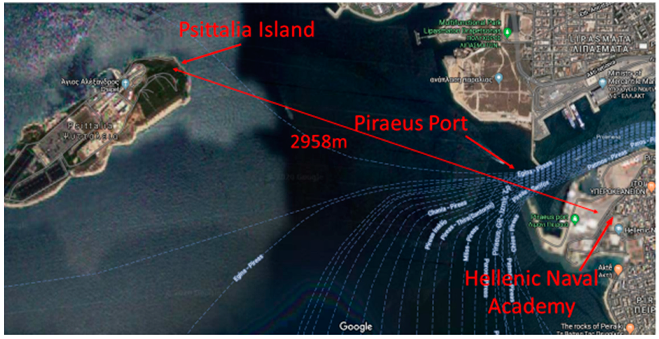
The experimental instrumentation was located on the roof of the Hellenic Naval Academy (HNA), i.e., primary terminal, and the lighthouse of Psitalia island, i.e., remote terminal. The horizontal optical link is located 35 m above the sea and crosses the entrance of the Piraeus port; nearly the entire path is over the water and, thus, clearly a maritime environment. Figure 1 shows the exact spots of both terminals in the map, as well as the ambient environment that the 2958-m-long optical link operates.

This link will be disrupted whenever a vessel taller than 35 m crosses the path; therefore, to minimize these disruptions, the experiment was carried out during the winter when fewer cruise ships visit. The FSO system used in the experiment was an MRV TS5000/155 model. The setup consisted of two terminals with operational characteristics available in

Table 2. Free space optical (FSO) System Parameters.

Parameter	Value
Operating Wavelength	850 nm
Light Source	3 Lasers
Total Output Power	150 mW
Beam Divergence	2 mrad
Detector Type	APD
FOV	2 mrad
Sensitivity	−46 dBm

. The system’s scheme used is intensity modulation/direct detection (IM/DD) and it operates in a data rate of 155 Mbps.

Both terminals utilized stand-alone PCs in order to send and receive/store data. The interface between them is achieved through an SFP multimode fiber cable, operating at 1310 nm, which drives the optical signal from the detector through an O–E converter directly to the PC. The RSSI data is then stored and is available to export for further analysis. The terminal over Psittalia island (Figure 2) can be remotely operated from the HNA through the optical link.

Additionally, an Ambient Weather (WS-2000) weather station is co-located with the HNA FSO terminal (Figure 3) to provide real time measurements of macroscopic meteorological parameters that include wind speed, wind direction, air temperature, relative humidity, air pressure, dew point, solar radiation and rainfall rate. These measurements are then stored and readily available to export, analyze and study.

4. Results and Analysis

The experimental measurements spanned over a period of two months, from 30 November 2019 until 31 January 2020. During the first part (30 November 2019–10 January 2020) the observed data were utilized to build the model. Due to technical reasons, the data collection during that period was not perpetual. During the second part, which consisted of two sub-periods (10–15 January 2020 and 24–31 January 2020), the model was validated against real data. The obtained data were stored and exported every few days for further analysis using spreadsheets and MATLAB. The location where the experiment took place, along with the diverse meteorological conditions, provided a very challenging environment for a laser communications link. During that period, the FSO link operated successfully in warm and sunny, rainy, cold and windy days. Therefore, the model was trained on a wide variety of conditions. Figure 4 and Figure 5 show the fluctuations of the observed meteorological parameters over the data collection period, including air temperature, dew point, relative humidity, air pressure, wind speed, solar radiation and rainfall rate.

Table 3. Collection of Mean, Minimum and Maximum observed values of meteorological parameters during the data collection period.

	Air Temperature (°C)	Dew Point (°C)	Relative Humidity (%)	Air Pressure (hPa)	Wind Speed (m/s)	Solar Radiation (W/m2)
Mean Value	14.07	8.3	69.34	1017.77	2.09	70.5
Min. Value	5.70	−4.9	32.00	990.70	0.00	0.0
Max. Value	22.20	14.7	94.00	1028.70	25.80	613.3

summarizes the mean, minimum and maximum values of the meteorological parameters observed during the data collection period.

4.1. Regression Model

A set of 25,056 data points (one measurement/minute) within a period of 42 days was utilized to deduce the empirical model for RSSI prediction. The following second-order polynomial has been selected to provide a good fit among seven independent parameters (wind speed, relative humidity, air temperature, air pressure, solar radiation, dew point and hourly rainfall rate) and the dependent RSSI,

$$\begin{array}{ll}RSSI=& -61236.1613-4.7678\times P+0.002386\times P^2+461.4112\times T-0.8294\times T^2\\ & -0.6145\times RH-0.0236\times R{H}^2+8.2251\times DP+0.2627\times D{P}^2-0.1626\times WS\\ & -0.011\times W{S}^2+0.04889\times SF-3.8313E-5\times S{F}^2-3.75634\times HR\end{array}$$

(8)

where T stands for the air temperature in Kelvin, P is the air pressure in hPa, RH is the percentage of relative humidity, DP is the dew point in Celsius, WS represents the wind speed in meters per second, SF being the solar flux in Watts per square meter and HR is the rain rate in mm/hour.

The newly derived model demonstrated a very decent accuracy with an R-squared of 68.2%. Figure 6 shows the predicted values of RSSI based upon the results of the regression analysis versus the observed one.

By using linear correlation coefficients, we further investigate the correlation coefficients of the considered parameters with RSSI. In the case under consideration, relative humidity appeared to have the most significant correlation with RSSI, with a negative value of −0.56557, indicative of its adverse effect to the link’s performance.

Table 4. Matrix of linear correlation coefficients for measured meteorological parameters and received signal strength from 30 November 2019 to 10 January 2020.

	Air Pressure	Air Temperature	Relative Humidity	Dew Point	Wind Speed	Solar Flux	Hourly Rain Rate	RSSI
Air Pressure	1	-	-	-	-	-	-	-
Air Temperature	−0.26383	1	-	-	-	-	-	-
Relative Humidity	−0.24084	0.234145	1	-	-	-	-	-
Dew Point	−0.31862	0.77857	0.788697	1	-	-	-	-
Wind Speed	−0.02946	−0.17976	−0.42763	−0.39007	1	-	-	-
Solar Flux	0.058201	0.279619	−0.33786	−0.04767	0.140114	1	-	-
Hourly Rain Rate	−0.26519	−0.02916	0.236718	0.117156	−0.01767	−0.04762	1	-
RSSI	0.13399	0.219768	−0.56557	−0.20549	0.131537	0.44691	−0.35769	1

summarizes the correlation coefficients of all seven parameters with RSSI.

Emphasis should be given to the impact of rain on the performance of the optical link. During the data collection period, i.e., totally 22.5 h, exhibited a non-zero precipitation rate, thus allowing further investigation on these effects. As shown in Table 4, the rain has a moderate anti-correlated relation (−0.35769) with RSSI. Additional analysis on MATLAB showed that a 32% of the total RSSI variance is explained by the variance of the hourly rain rate, i.e., R-squared in Figure 7.

4.2. Model Validation

The validation period of the first model was from 10–15 January 2020. During this period, in general, the range of the observed parameters is smaller than the data collection period, the mean air temperature is 3 degrees lower, and the mean air pressure was more than 7 hPa higher. Qualitatively, the modeled RSSI estimations Equation (8), as seen in Figure 8, demonstrated a very good fit with the observed values with a few exceptions where the observed values exhibited strong fluctuations. In this part, the model predicted a smoother form with less fluctuations. Quantitatively, the observed RSSI values as compared to the predicted values for this period had an R-squared of 76%. The percentage of the predicted values variance is explained very well by the variance of the observed values: that is the R-squared reached a value of 69%. The model also correlated very well with a linear correlation coefficient of 0.8327. Apart from the modeled and observed values graph, Figure 8 shows the RSSI values graph predicted by the model proposed in [17] and Equation (6) by J. Latal et al. A relatively significant constant offset of approximately 80–100 RSSI units is observed during the entire period. It should be pointed out that the model proposed by J. Latal et al. [17] referred to a terrestrial terrain in contrast with our model, which focuses on a maritime environment.

The second validation period was from 24 to 31 January 2020. During this period, the mean values as well as the range of the observed parameters were closer to those of the data collection period. Qualitatively, the modeled RSSI estimations (Equation (8)), as seen in Figure 9, again yielded a very good match with the observed values. It lacked accuracy on the parts where observed RSSI values exhibited abrupt “peaks”. In these parts, the model seemed to follow better the peak values of the observations. Quantitatively, the observed RSSI values, as compared to the meteorological parameters of this period, had an even better R-squared (84%). The percentage of the predicted values variance is also explained better by the variance of the observed values, that is the R-squared, reached a value of 74%. The model also correlated very well with the observed values with a linear correlation coefficient of 0.8645. Finally, the model proposed in [17] and Equation (6) had an even larger offset which at some points reached values of around 100–120 RSSI units.

4.3. Refractive Index Structure Parameter Empirical Models

The same two periods reported in the previous section have been used to estimate the refractive index structure parameter strength. Even though the experimental instrumentation did not include a scintillometer for the collection of real values, the two empirical models, i.e., Equations (5) and (6), were utilized to obtain approximations to compare those with RSSI observations. Both models were coded in MATLAB, and $C_n^2$ predictions have been deduced by utilizing the same set of meteorological parameters. Therefore, there is inherently a relation between $C_n^2$ and RSSI. Figure 10 and Figure 11 show the $C_n^2$ parameter fluctuations for each period.

The general bell shape of the diurnal profile of $C_n^2$ is easily recognized in Figure 10 and Figure 11. The lower values occurred right before sunrise and after sunset, whereas the maximum values occurred around noon. Model 1 exhibited a more extended range of values, with lower minimum and higher peak values. Peak values coincided in both models. An important characteristic to notice is the relatively short range of $C_n^2$ diurnal fluctuations, which even in model 1 case is approximately one order of magnitude. Numerical values of $C_n^2$ have also been obtained from the Huffnagel-Valley model, yielding 9 × 10⁻¹⁵ m^−2/3. This value is slightly lower than the means of models 1 and 2, as shown in

Table 5. Empirical Models for $C_n^2$ comparison for periods 10–15 January and 24–31 January 2020.

	Min. Value (m−2/3)	Max. Value (m−2/3)	Mean Value (m−2/3)
Model 1 (10–15 January 2020)	1.6 × 10−15	2.78 × 10−14	1.31 × 10−14
Model 1 (24–31 January 2020)	7.166 × 10−15	2.985 × 10−14	1.47 × 10−14
Model 2 (10–15 January 2020)	1.159 × 10−14	2.58 × 10−14	1.8728 × 10−14
Model 2 (24–31 January 2020)	1.5398 × 10−14	2.7 × 10−14	1.9878 × 10−14
Huffnagel-Valley	9.02 × 10−15 m−2/3

, below.

The R-squared parameter and correlation coefficient between observed and modeled RSSI with modeled $C_n^2$ are summarized in

Table 6. Summary of R-squared (Correlation Coefficients) for Observed and Modeled Received Signal Strength Indicator (RSSI) with ${\mathit{C}}_{\mathit{n}}^{\mathbf{2}}$ for both empirical models.

	${\mathit{C}}_{\mathit{n}}^{\mathbf{2}}$ Model 1	Cn2 Model 2
Observed RSSI (10–15 January 2020)	44.10% (0.65425)	40.50% (0.63630)
Modelled RSSI (10–15 January 2020)	73.97% (0.78042)	64.79% (0.77280)
Observed RSSI (24–31 January 2020)	23.10% (0.46870)	17.89% (0.42000)
Modelled RSSI (24–31 January 2020)	46.36% (0.61640)	42.24% (0.64820)

. The first period for the observed RSSI exhibited moderate R-squared parameter, whereas the modeled RSSI presented a considerably improved R-squared and also significant correlation. The second period resulted in slightly worse R-squared and correlation coefficient.

4.4. Distribution Fitting Analysis

The Kullback-Leibler (KL) divergence provides a very useful mathematical tool to measure the difference of two probability distributions [26]. KL divergence is a non-symmetric measure between two probability distributions p(x) and q(x). The KL divergence, denoted Kullback-Leibler Divergence, DKL (p(x) || q(x)), represents the information lost: the smaller the KL divergence, the more the two distributions are similar. In case of a discrete random variable x, assume two probability distributions p(x) and q(x), both non-negative and both summing up to unity for any x in X. The definition of KL divergence is then [26],

$$D_{KL}(p(x)||q(x))={\displaystyle \sum _{x\in X}^{}p(x)\ln \frac{p(x)}{q(x)}}$$

(9)

Typically, p(x) represents the “true” or a theoretical calculated distribution of the observed data, whereas q(x) represents a model or an approximation of p(x). In case of a continuous variable x, then

$$D_{KL}(p(x)||q(x))={\displaystyle \underset{-\infty }{\overset{\infty }{\int }}p(x)\ln \frac{p(x)}{q(x)}dx}$$

(10)

Based on the KL divergence theory, the theoretical distribution that best fits the observed RSSI data during the collection period (30 November 2019–10 January 2020) has been deduced. Utilizing the distribution fitting application of MATLAB, initially we estimated the parameters of the probability density function of three theoretical distributions, namely lognormal, Weibull and gamma, for the considered RSSI values range, i.e., min. 331–max. 512. The empirical PDF of the RSSI data has also been evaluated and the corresponding results are available both graphically in Figure 12 and numerically in

Table 7. Divergence for Gamma, Lognormal and Weibull probability distributions.

	DKL (p(x)||q(x))
Gamma	4.17 × 10−2
Lognormal	4.38 × 10−2
Weibull	7.95 × 10−2

. From Table 7, it becomes evident that among the three considered probability distributions, the gamma distribution yields the best fit, a fact that is difficult to be ascertained from an inspection of Figure 12.

5. Conclusions

In this paper, we proposed a new mathematical model to predict the received signal strength of an FSO optical link. The model has the form of a second-order polynomial with seven macroscopic meteorological parameters as the independent variables. An optical communications link over a maritime environment and a weather station provided the required data. The predicted RSSI values fitted the observed values quite well, yielding an R-squared value of 68.2%. The correlation of all seven parameters to the RSSI has been calculated to deduce the weight of each one’s effect. Emphasis has been given to the rain effect, where 32% of the RSSI variance was explained by the rainfall rate variance (R-squared = 0.32). The proposed model has been validated against real data in two separate periods and the R-squared and correlation coefficient between the observed and modeled RSSI values has been computed to check how good the fit was. Both periods exhibited high R-squared and correlation coefficient, namely 69% and 0.8327, respectively. Two empirical models have been utilized to estimate the $C_n^2$ parameter for the same periods and its relationship with RSSI has been explored. Finally, the KL divergence was used to compare the goodness of fit for different probability distributions, i.e., gamma, lognormal and Weibull to the RSSI data probability distribution, and the gamma distribution yielded the best fit. Experimenting with a laser link in the open sea for extended periods of time is not trivial, therefore we utilized an established link between two fixed points on land that crosses a maritime environment and allows for adequate experimental data to be obtained in order to build our model. Therefore, our model allows the prediction of a maritime optical link with the utilization of a single point measurement system for atmospheric parameters.

References

1. Perram, G.P.; Cusumano, S.J.; Hengehold, R.L.; Fiorino, S.T. Introduction to Laser Weapon Systems, 1st ed.; Directed Energy Professional Society: Albuquerque, NM, USA, 2010. [Google Scholar]
2. Ghassemlooy, Z.; Popoola, W.O. Terrestrial Free-Space Optical Communications. In Mobile and Wireless Communications Network Layer and Circuit Level Design; Fares, S.A., Adachi, F., Eds.; Books on Demand: Metro Manila, Philippines, 2010; pp. 355–392. [Google Scholar]
3. Andrews, L.C.; Phillips, R.L.; Hopen, C.Y. Laser Beam Scintillation with Applications, 2nd ed.; SPIE: Bellingham, WA, USA, 2001. [Google Scholar]
4. Majumdar, A.K. Free-space laser communication performance in the atmospheric channel. J. Opt. Fiber Commun. 2005, 2, 345–396. [Google Scholar] [CrossRef]
5. Moore, C.I.; Burris, H.R.; Stell, M.F.; Wasiczko, L.; Suite, M.R.; Mahon, R.; Rabinovich, W.S.; Gilbreath, G.C.; Scharpf, W.J. Atmospheric turbulence studies of a 16-km maritime path. In Proceedings of the SPIE 5793, Atmospheric Propagation II, Orlando, FL, USA, 25 May 2005. [Google Scholar]
6. Wasiczko, L.M.; Moore, C.I.; Burris, H.R.; Suite, M.; Stell, M.; Murphy, J.; Gilbreath, G.C.; Rabinovich, W.; Scharpf, W. Characterization of the Marine Atmosphere for Free-Space Optical Communication. In Proceedings of the SPIE 6215, Atmospheric Propagation III, Orlando (Kissimmee), FL, USA, 17 May 2006. [Google Scholar]
7. Grant, K.J.; Mudge, K.A.; Clare, B.A.; Perejma, A.S.; Martinsen, W.M. Maritime Laser Communications Trial 98152-19703. Command, Control, Communications and Intelligence Division; DSTO: Edinburgh, Australia, 2012. [Google Scholar]
8. De Jong, A.N.; Schwering, P.B.W.; van Eijk, A.M.G.; Gunter, W.H. Validation of Atmospheric propagation models in littoral waters. Opt. Eng. 2013, 52. [Google Scholar] [CrossRef] [Green Version]
9. Moore, C.I.; Suite, M.R.; Murphy, J.L.; Tugman, J.E.; Ferraro, M.S.; Wade, T.; Mahon, F.R.; Goetz, P.G.; Rabinovich, W.S.; Burris, H.R.; et al. MIO Tar2host Lasercomm Experiment in Trident Warrior 08. In Proceedings of the 2008 IEEE Antennas and Propagation Society International Symposium, San Diego, CA, USA, 5–11 July 2008. [Google Scholar]
10. Alheadary, W.G.; Park, K.-H.; Alfaraj, N.; Guo, Y.; Stegenburgs, E.; Ng, T.K.; Ooi, B.S.; Alouini, M.-S. Free-space optical channel characterization and experimental validation in a coastal environment. Opt. Express 2018, 26, 6614–6628. [Google Scholar] [CrossRef] [PubMed] [Green Version]
11. Alheadary, W.G.; Park, K.-H.; Ooi, B.S.; Alouini, M.-S. Free-space optical channel characterization in a coastal environment. J. Commun. Inf. Netw. 2017, 2, 100–106. [Google Scholar] [CrossRef] [Green Version]
12. Michael, S.; Parenti, R.R.; Walther, F.G.; Volpicelli, A.M.; Moores, J.D.; Murphy, R.W.W., Jr. Comparison of Scintillation Measurements from a 5 km Communications Link to Standard Statistical Models. In Proceedings of the SPIE 7324, Atmospheric Propagation VI, Orlando, FL, USA, 2 May 2009. [Google Scholar]
13. Bourazani, D.; Stasinakis, A.N.; Nistazakis, H.E.; Varotsos, G.K.; Tsigopoulos, A.D.; Tombras, G.S. Experimental Accuracy Investigation for Irradiance Fluctuations of FSO Links Modeled by Gamma Distribution. In Proceedings of the 8th International Conference from Scientific Computing to Computational Engineering, Athens, Greece, 4–7 July 2018. [Google Scholar]
14. Kampouraki, M.N.; Stasinakis, A.N.; Nistazakis, H.E.; Tsigopoulos, A.D.; Tombras, G.S.; Chronopoulos, G.G.; Fafalios, M.E. Experimental and Theoretical Bit Rate Estimation of Turbulent FSO Link Over the Maritime Area at Piraeus Port. In Proceedings of the 6th International Conference from Scientific Computing to Computational Engineering, Athens, Greece, 9–12 July 2014. [Google Scholar]
15. Tunick, A. Statistical analysis of optical turbulence intensity over a 2.33 km propagation path. Opt. Express 2007, 15, 3619–3628. [Google Scholar] [CrossRef] [PubMed]
16. Tunick, A.; Nikolay, T.; Mikhail, V.; Gary, C. Characterization of Optical Turbulence (Cn2) Data Measured at the ARL A_LOT Facility; Technical Report for U.S. Army Research Laboratory: Adelphi, MD, USA, September 2005. [Google Scholar]
17. Latal, J.; Vitasek, J.; Hajek, L.; Vanderka, A.; Koudelka, P.; Kepak, S.; Vasinek, V. Regression Models Utilization for RSSI Prediction of Professional FSO Link with Regards to Atmosphere Phenomena. In Proceedings of the 2016. International Conference on Broadband Communications for Next Generation Networks and Multimedia Applications (CoBCom), Graz, Austria, 14–16 September 2016. [Google Scholar]
18. Latal, J.; Hajek, L.; Vanderka, A.; Vitasek, J.; Koudelka, P.; Hejduk, S. Real Measurements and Evaluation of the Influence of Atmospheric Phenomena on FSO Combined with Modulation Formats. Electronics 2016, 20. [Google Scholar] [CrossRef] [Green Version]
19. Hajek, L.; Vitasek, J.; Vanderka, A.; Latal, J.; Perecar, F.; Vasinek, V. Statistical prediction of the atmospheric behavior for free space optical link. In Proceedings of the SPIE 9614, Laser Communication and Propagation through the Atmosphere and Oceans IV, San Diego, CA, USA, 4 September 2015. [Google Scholar]
20. Andrews, L.C.; Phillips, R.L. Laser Beam Propagation through Random Media, 2nd ed.; SPIE Optical Engineering Press: Bellingham, WA, USA, 2005. [Google Scholar]
21. Oermann, R.J. Novel Methods for the Quantification of Atmospheric Turbulence Strength in the Atmospheric Surface Layer. Ph.D. Thesis, School of Chemistry and Physics, University of Adelaide, Adelaide, SA, Australia, 2014. [Google Scholar]
22. Nistazakis, H.E.; Katsis, A.; Tombras, G.S. On the Reliability and Performance of FSO and Hybrid FSO Communication Systems over Turbulent Channels; Nova Science Publishers: Hauppauge, NY, USA, 2011; pp. 69–112. [Google Scholar]
23. Sabot, D.; Kopeika, N.S. Forecasting optical turbulence strength on the basis of macroscale meteorology and aerosols: Models and validation. Opt. Eng. 1992, 31. [Google Scholar] [CrossRef]
24. Lionis, A.; Cohn, K.; Pogue, C. Experimental Design of a UCAV-based High Energy Laser Weapon. Master’s Thesis, Naval Postgraduate School, Monterey, CA, USA, December 2016. [Google Scholar]
25. Rabinovich, W.S.; Moore, C.I.; Mahon, R.; Goetz, P.G.; Burris, H.R.; Ferraro, M.S.; Murphy, J.L.; Thomas, L.M.; Gilbreath, G.C.; Vilcheck, M.; et al. Free-space optical communications research and demonstrations at the U.S. Naval Research Laboratory. Appl. Opt. 2015, 54, 189–200. [Google Scholar] [CrossRef] [PubMed]
26. Kullback, S.; Leibler, R.A. On information and sufficiency. Ann. Math. Stat. 1951, 22, 79–86. [Google Scholar] [CrossRef]
Figure 1. The laser communications link located across Piraeus harbor entrance.
Electronics 09 01109 g001
Figure 2. The FSO link from the Psitalia Island point of view.
Electronics 09 01109 g002
Figure 3. The MRV TS5000/155 FSO system on the Hellenic Naval Academy and the co-located ambient weather WS-2000, weather station.
Electronics 09 01109 g003
Figure 4. Air Temperature, Dew Point and Relative Humidity fluctuations over the data collection period.
Electronics 09 01109 g004
Figure 5. Air Pressure, Wind Speed and Solar Radiation fluctuations over the data collection period.
Electronics 09 01109 g005
Figure 6. Comparison between observed and modeled RSSI for the data collection period.
Electronics 09 01109 g006
Figure 7. Versus hourly rainfall rate measured data.
Electronics 09 01109 g007
Figure 8. Model evaluation for measured RSSI data for the period 10–15 January 2020. The grey line shows the literature modeled RSSI proposed by J. Latal et al. [17].
Electronics 09 01109 g008
Figure 9. Model evaluation for measured RSSI data for the period 24–31 January 2020. The grey line shows the literature modeled RSSI proposed by J. Latal et al.
Electronics 09 01109 g009
Figure 10. C n 2 parameter for empirical models over the period 10–15 January 2020.
Electronics 09 01109 g010
Figure 11. C n 2 parameter for empirical models over the period 24–31 January 2020.
Electronics 09 01109 g011
Figure 12. PDF fits of gamma, lognormal and Weibull distributions for observed RSSI data for the time period from 30 November 2019 to 10 January 2020.
Electronics 09 01109 g012