1. Introduction
Hardware-based control systems are required in certain environments, when perfect synchronization is compulsory. In this work we present and compare the implementation of jitter-free synchronization in research facilities using two methods: a tool that allows the automated synthesis of hardware control systems based on graphical statechart descriptions and a microprogrammed architecture [
1] for the same statechart. The statechart descriptions follow a constrained version of SCXML [
2] tailored to hardware systems, and are also compared to the implementations developed by a skilled engineer not only in terms of the generated code, but also in relation to the ease and speed of support, maintainability and upgradability of those implementations in deployments with certain requirements such as research facilities. We will focus on the specific case that motivated this work, which is the generation of triggering signals in a particle accelerator at the European Spallation Source (ESS) [
3].
Statecharts were introduced by Harel in [
4] as a tool to implement complex control systems, either in software or hardware. They may be seen as an extension of Finite State Machines (FSMs) that allow a clear specification of hierarchy and concurrency. These diagrams allow to group basic states into super-states and specify conditions and transitions at a super-state level, reducing the complexity of the specification and improving the readability. Some states may be active concurrently, making them suitable to describe complex real-world systems, and the conditions to enable or disable them can be specified in an unambiguous manner. Therefore, statecharts largely improve FSMs, and they become part of the Unified Modeling Language (UML) [
5].
Whereas automated software synthesis of statecharts is supported by several tools [
6,
7,
8], only a few efforts have been made towards hardware synthesis of statecharts. A number of tools, most of them discontinued, provided partial solutions, but in general not all the functionalities in statecharts are implemented, specially history. A thorough literature review of hardware synthesis of statecharts is described in
Section 2 together with an introduction to statecharts.
Section 3 presents how an engineer would tackle the HDL specification of a statechart, and
Section 4 a description of the hardware synthesis tool, listing the techniques that allow to synthesize statecharts. In
Section 5 the description of the microprogrammed architecture and the procedure to write the microcode that implements the statechart is also presented. Finally, in
Section 6 the code obtained from all methods is compared, focusing on the application of these methods to the ESS case, and in
Section 7 the conclusions of this work are presented.
2. Statecharts
Statecharts were introduced in 1987 as a tool to overcome the limitations of FSMs [
9,
10] in describing the behaviour of complex systems. FSMs are state-based models where only one state is active at any given time, which can be changed by external inputs or internal conditions. The change between states is called transition.
The aspect that limits the usability of FSMs is that they can greatly grow in complexity when adding states. Statecharts deal with this issue by extending the conventional state-transition diagrams allowing for hierarchy and nested states, concurrency of parallel states and better communication among the states. This allows for more compact, expressive and modular diagrams, that can describe complex behaviour with smaller diagrams when compared to FSMs. As such, statecharts are a visual formalism for describing states and transitions. At the same time statecharts maintain all of the characteristics of FSMs, such as conditions, outputs, etc. Their main contributions are:
Orthogonality: as opposed to classical FSMs, where only one state can be active at a time, statecharts can have more than one state active concurrently. These are called AND-states, while the traditional approach are called OR-states. Orthogonality is very useful for describing subsystems.
Depth: there is a hierarchy in the state structure, allowing for states or even complete FSMs or sub-statecharts to live inside other states, connected with inter-level transitions. In the nested structure the state containing other states is called super-state. Depth allows for great modularity, clustering, and ease of movement between levels of abstraction by zooming in or out. It is also possible to define initial and default initial states, and have history in the states, as explained in
Section 4.2.3.
Broadcast mechanism: the different parts of a statechart are not independent of each other. An action taking place in one part of the statechart can cause many different actions in a completely different part of the statechart taking into account the orthogonality and depth. To allow this it may be necessary that many components communicate with each other even if it is not evident in the specification of the statechart.
In
Section 4.2 the features of statecharts are explained in more detail.
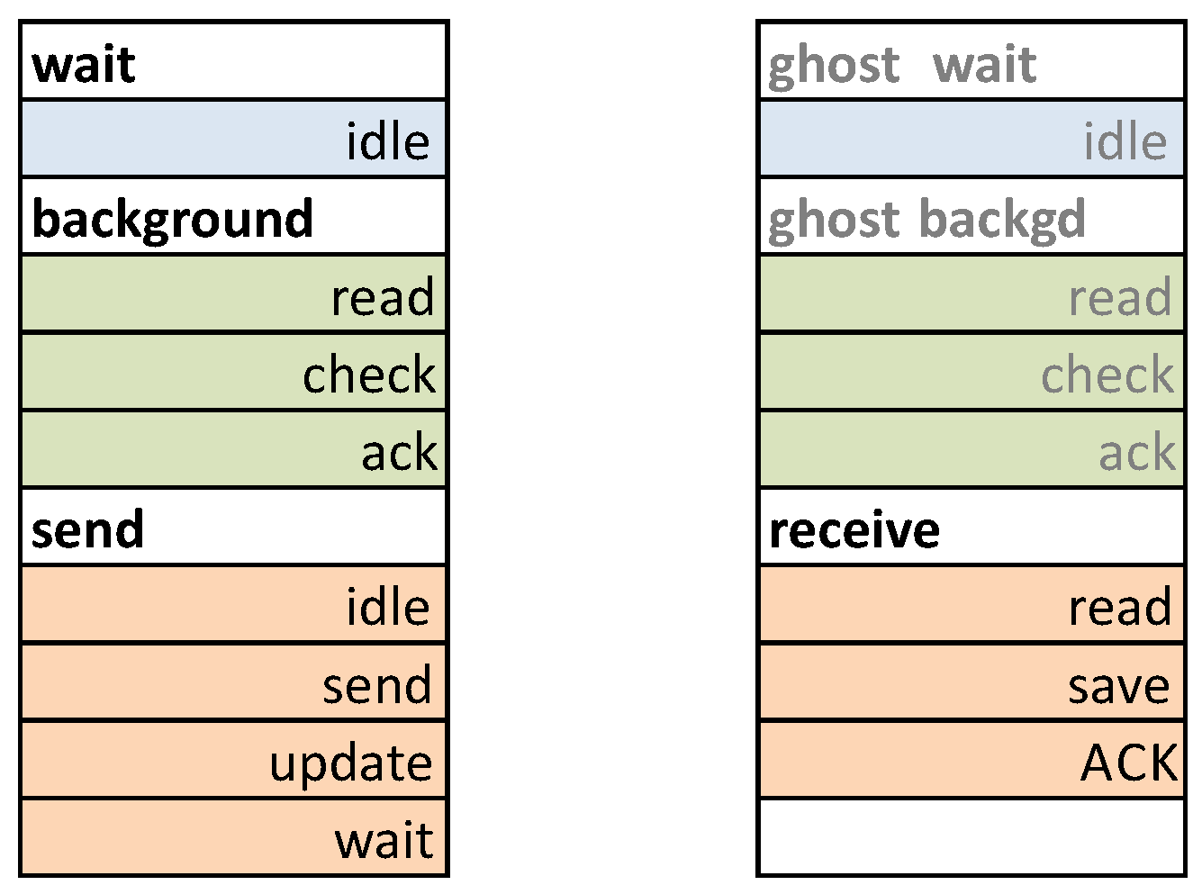
In
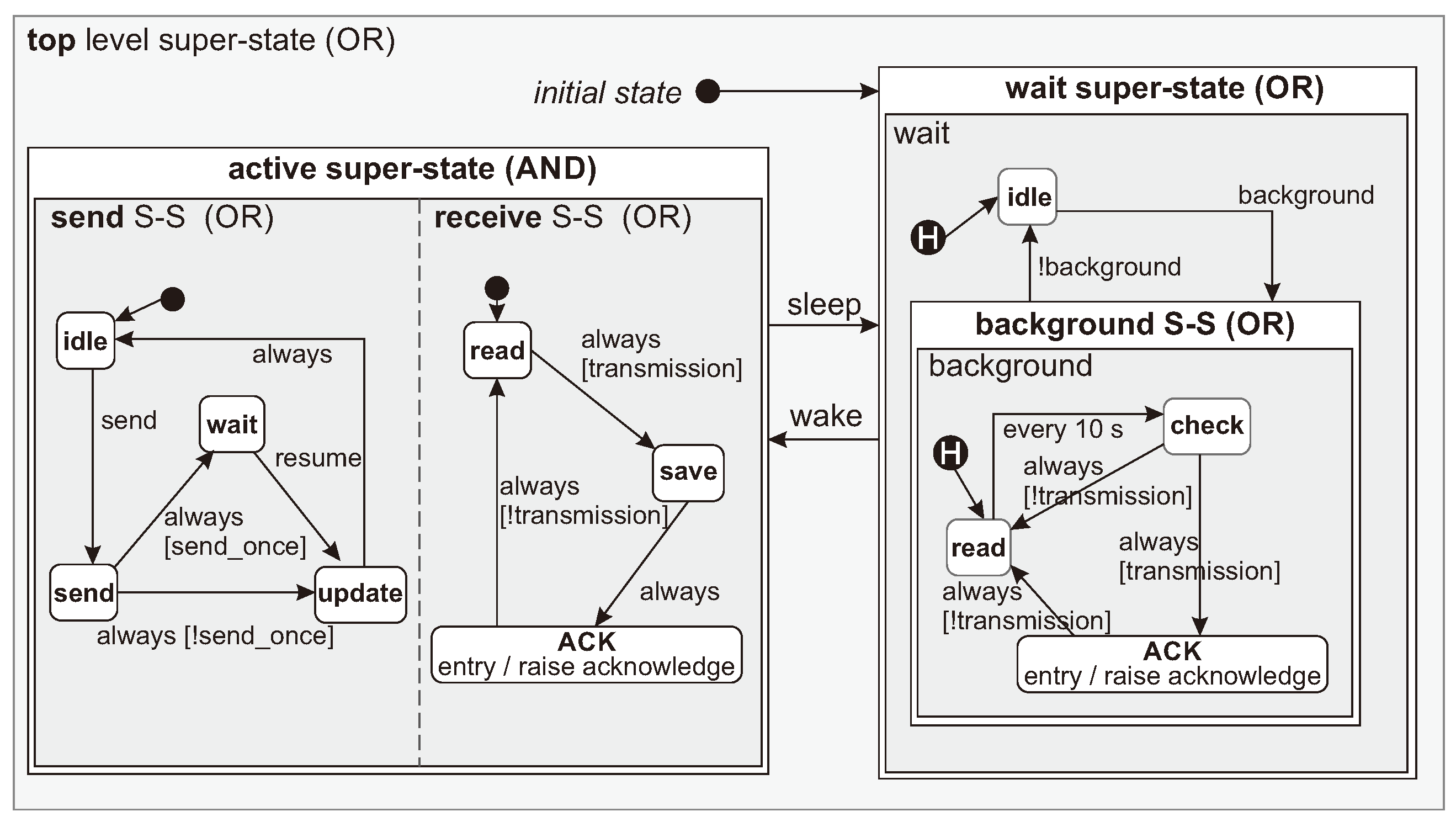
Figure 1, a statechart is shown. At the higher level, top is an OR super-state, because either active OR wait super-states must be running, but not both at the same time. The active super-state is made up of two regions, send and receive. This illustrates the concept of hierarchy, as one super-state may be made up of several ones. In this case, both super-states are running in parallel, allowing to describe concurrent processing. This is called an AND super-state (denoted by the divider line). Inside each of them, only one state is active (e.g., update and save working concurrently). Contrarily, when wait is active, either idle or background are running, but not both at the same time. A black dot and an arrow point at the initial node for each super-state. Moreover, two super-states are denoted to have history (an H within the dot). Therefore when processing returns to wait, it remembers whether it was running in idle or background and, in the latter case, in which of the three nodes. History is a crucial characteristic that is seldom supported in previous works.
Review on Hardware Synthesis
Soon after statecharts were proposed, a number of tools for hardware synthesis were developed. However, most of them were limited in scope, or were based on now obsolete technologies. In 1989, Drusinsky and Harel [
11] studied the challenges related to defining history and activation and deactivation of super-states. The work gives implementation hints focused on Programmable Logic Arrays (PLAs). Drusinksy and Yoresh [
12] analysed the limitations of the previous work, and focused on reducing the complexity of the transitions between super-states and efficient state-coding. Again, the solutions are mainly oriented to PLA implementations. The first reference to an automated tool is found in [
13], where a tool called I-Logix Express VHDL (Very High Speed Integrated Circuit Hardware Description Language) is used. However, it does not cover most of the statechart features, and the paper is mainly a description of some use cases. Another paper [
14] using the same tool focusses mainly on validation, and overlooks implementation aspects, such as history. A later product by I-Logix (Statemate) supported hardware synthesis with some limitations. Although I-Logix has produced more statechart software synthesis tools, such as Rhapsody (now owned by IBM), hardware synthesis was not included in them.
In [
15], a comparison is made on the complexity of implementing the system directly in VHDL code versus modelling and synthesizing the statecharts with the help of SPeeDCHART. Despite the advantages of using a graphical environment, the authors highlight that strong VHDL knowledge is still required. The same authors published a similar comparison based on implementing fuzzy control systems. Nevertheless, the provided examples are actually implemented as FSMs, as they lack of the sophistication of real statecharts. In [
16], an Application-Specific Instruction Set Processor (ASIP) is proposed for mapping statecharts. Most of the paper focuses on the architecture of the ASIP. Statecharts are analysed using a tool called ROOM. History and other features are not supported. In a later work [
17], this limitation is not solved. A methodology for co-design is shown where statecharts are implemented in hardware as flattened FSMs. Furthermore, in [
18] the implementation of datapaths ruled by a FSM or statechart is studied. The latter is implemented using SPeeDCHART (which was also used in [
15] and [
19]), and the analysis reveals that the tool does not implement concurrency in a satisfactory manner. Moreover, hierarchical superstates are flattened, rendering a single superstate with a large number of states. The authors do not mention how they deal with history.
More recently, Qin, Chin et al. have published a number of papers [
20,
21] that analyse the theoretical basis of automatic conversion from statecharts to Verilog HDL. Moreover, in [
22], they introduce a statechart editor and a hardware mapping tool for which some implementation examples are provided. The applicability of these works is limited by the fact that they do not support history nor transitions between states at different levels.
In [
23], a methodology is presented for generating SystemC and VHDL code from a statechart specification. Much of the paper is devoted to explain how to guarantee consistency between SystemC and VHDL code behaviour when triggering events during simulation. The paper is mostly focused on SystemC, so little details are given on the generation of VHDL code. Furthermore, as in many other works, history is not supported.
Finally, Mathworks includes Stateflow [
6], a commercial toolbox for Matlab that supports the statecharts formalism, including history in nested regions. An add-on to the same product called HDL Coder produces usable code for over 200 hardware platforms.
In summary, there is still a need for synthesis tools as the other existing tools, with the exception of a commercial one, cover only a partial set of features and most of them are now discontinued.
3. Hardwired Strategy
Following there is an explanation of how an engineer would implement a statechart by hand. Using an HDL such as Verilog or VHDL, the starting point consists of defining a process for each leaf superstate. That is, those that do not contain other superstates. Each of those processes encode a FSM with as many states as there are in each superstate. Moreover, a registered activation bit is defined for each of them. The code for every process checks the activation bit. If active, a switch-case construct will be used to write code for each basic state, which may include: generating outputs, updating the internal state, producing events (signals) for other processes and switching off the current superstate and sending an enabling event to a different one.
Inactive superstates evaluate if the conditions to be enabled are fulfilled. In such a case, the activation bit will be switched on. Hierarchy is not implemented by nesting processes, but by the way in which events are produced and consumed by the different processes. Looking at
Figure 1, event wake will activate both send and receive. There is not a process for superstate active. Furthermore, sleep will be processed by all the superstates. First, send and receive will become inactive.
Moreover, the internal state will be recovered if history is implemented or, otherwise, reset. In some cases, a superstate may become active or inactive under different events. Thus, some processes must register additional information that enables the code to decide when and how to activate the superstate. This is sometimes called deep history. As an example, wait/idle will activate itself only if it was disabled by wake, but not by background. Similarly, background will decide whether it should resume or not.
Most of the communications between processes are carried out using events (signals). In some cases, an event or an output may be produced by different processes. In such a case, all the sources are or-ed to produce an unified event or output. Hence, inactive processes must produce zero-valued outputs and events. Beside the superstates, additional processes could be defined in order to produce and/or consume specific events. This includes all kind of counters or alarm triggers.
In summary, the well-known methodology for synthesizing FSMs must be extended with the addition of an on/off bit. Furthermore, a simple mechanism for implementing history is needed; and hierarchy is modelled by raising and consuming events. It must be remarked that all processing is specified with a clock cycle granularity. Therefore, actions and transitions must be completed in the duration of a clock cycle. Those actions that may span several cycles (such as iterations) could require splitting into different states.
5. Microprogrammed Architecture
A microprogrammed architecture [
1] for statecharts is now described. The basic element of this architecture is a circuit able to run one or more superstates in a non-concurrent manner. The circuit is able to switch between superstates connected by transitions and implement shallow history.
In order to implement the concurrency required by AND-superstates, as many of those circuits must be instantiated as superstates may run in parallel at the same time. Each circuit is made of a micro-memory that stores one micro-instruction for each basic state. Each micro-instruction encodes the actions to be carried out by that state, and all the possible transitions and the conditions (event) that would trigger those transitions. The circuit will read one micro-instruction each cycle using a program counter (PC), decode it, execute the actions, and select the next value for PC after evaluating the list of conditions and transitions.
All instances have access to the same set of inputs, outputs and internal variables. Events derived from inputs and variables influence the transitions on different instances, establishing connections between superstates. For example, one superstate may change a common variable in order to trigger an event in another concurrent one. In the following paragraphs, the implementation is described in detail.
Each instance is made of the following elements: micro-memory, PC, a set of registers to implement history, the logic to decode and evaluate the conditions and transitions, and the logic to decode the actions to be performed. At least, as many instances are needed, as concurrent superstates but, in order to enable future upgrades, a slightly larger number is recommended. The use of double-port memories allows sharing part of the cost between instances, especially when each of them implements only a few states. The length of the micro-instructions may be significantly large, especially in cases with many inputs and/or variables and outputs. Therefore, several memory modules are often required for each instance, and the advantage of sharing becomes more evident.
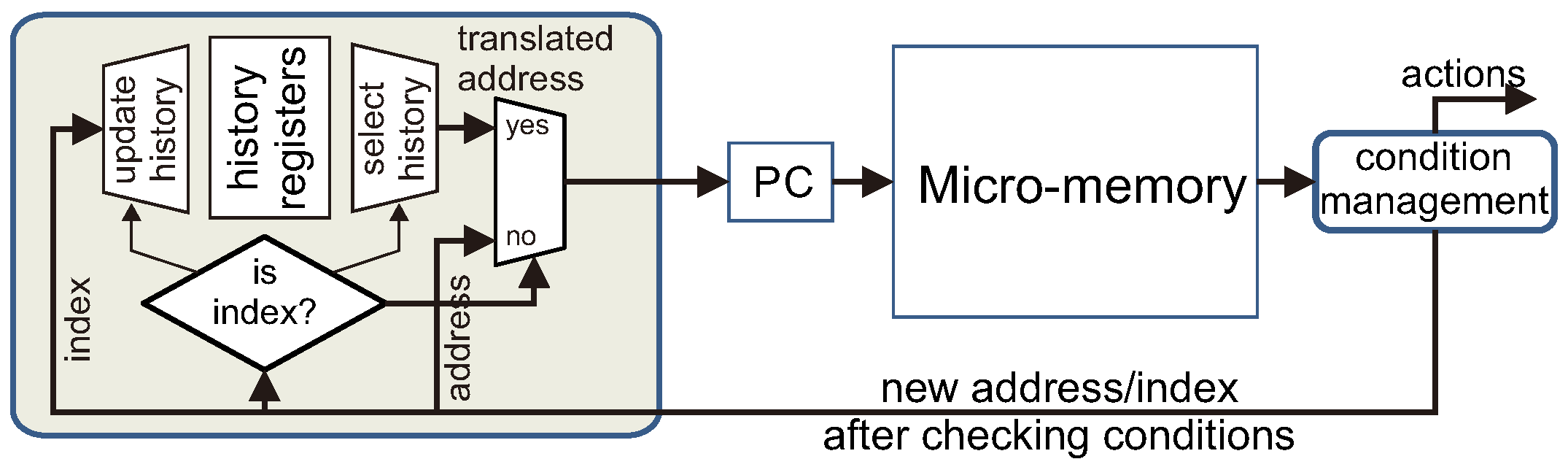
The program counter represents addresses in the micro-memory, but this may require a translation in some cases. Thus, when switching to a new state within the same superstate, the microinstruction provides the exact address of the next state. However, when switching to a different superstate, a special code is given instead. That code is an index in the range of 0 to 7, for example, and it is translated to a real address using the history register at that index. Thus, the first addresses are reserved and any transition to one of those addresses is translated to a real one. At the same time, if that superstate implements history, the current content of PC is stored in the history register of the current superstate. In this way, future transitions back to the exiting superstate will resume at the right state/micro-instruction. The initial values for the history registers are loaded at configuration time, at the same time as the content of the micro-memory, and a set of flags that signal whether each superstate implements history or not.
Figure 3 shows how micro-memories, PC, and history registers work together.
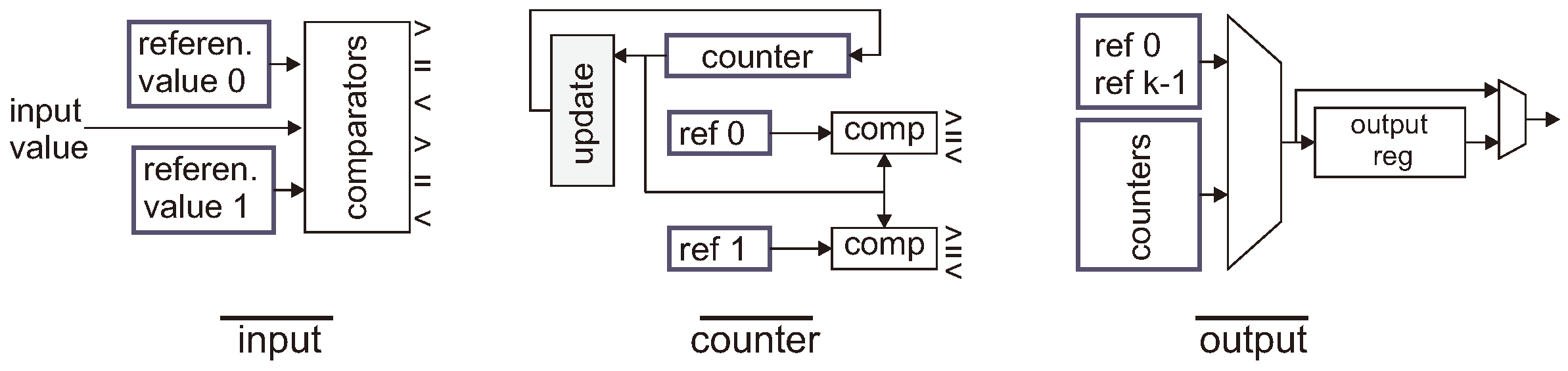
Inputs to the system are key in decision making. Events based on inputs are produced by comparing each input value to a set of reference values (we propose 2 for each input). Hence, events such as input1 is lower than ref1 can be used as conditions for any of the running microprograms.
Counters are used as internal variables. The value of each counter is also compared to reference values producing events similarly to inputs. A micro-instruction may update the content of any counter by issuing a command that specifies loading or adding a reference value, incrementing or decrementing it.
Finally, outputs are selected by the micro-programs assigning one of the counters or a predefined value. Optionally, each individual output may be configured to be registered.
Figure 4 shows the basic structure of the three types of components.
In order to deal with a mix of OR and AND superstates, all the microprograms run concurrently, even if no real work is done. Hence, a microprogram may be running a ghost superstate until it branches into an activated AND superstate. Ghost superstates are made of micro-instructions that evaluate the conditions that may lead to branch to another superstate, but they do not change any internal variable or produce any output.
Figure 5 shows how to implement the complete statechart in
Figure 1 using two microprograms. The second one will mimic all branches until arriving to receive, where real actions will be carried out. The same scheme may be applied for a larger number of micro-programs and deeper hierarchies.
It is not possible to implement deep history using the proposed architecture, as it does not implement call-return, just branching. Hence, the engineer must choose a fixed superstate to return to. However, each superstate history is not lost, so that when entering that superstate, execution will resume at the right micro-instruction.
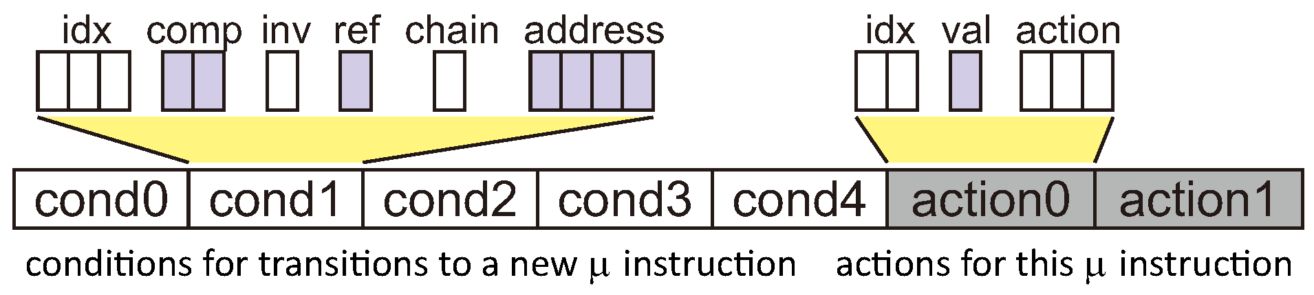
5.1. Micro-Instruction Format
Micro-instructions are made of two fields. First, a set of conditions to decide where to branch. Each condition is made of: the index of the event to be evaluated; a comparison (
); inverting flag; the reference value to use; the chain bit; and the target address. Simple conditions may be combined (and operand) by setting the chain bit. The or operand is implemented by using the same target for different conditions. The second field specifies the actions to be taken: updating one or more counters or producing a given output.
Figure 6 shows the format for the statechart in
Figure 1. Allowing several conditions increase micro-instruction length, but limiting the number requires splitting the evaluation.
Figure 7 shows an example, when the format is so narrow that only two conditions may be encoded in the same micro-instruction. In such cases, engineers must assess the impact of using extra cycles.
5.2. Configuration
A chain of registers store the initial addresses for each superstate; the flags that support history; the reference values for the inputs, counters and outputs; and the initial values of the counters. The configuration is loaded byte by byte and it propagates to the last element in the chain, where the micro-memories are located.
6. Evaluation
The proposed methods are now evaluated using four different use cases: the example from
Figure 1, the digital watch proposed by Harel in his original work [
4] and the two main components of the ESS timing system—the event generator (EVG) and the event receiver (EVR)—which provides the fast and jitter-free synchronization that is required to successfully run such a complex machine as ESS. Hence, one engineer introduced the diagrams in Yakindu and used our tool to produce VHDL code in an automatic way and implemented the statecharts. A second engineer analysed the statecharts and produced VHDL code by hand and implemented them using the microprogrammed architecture.
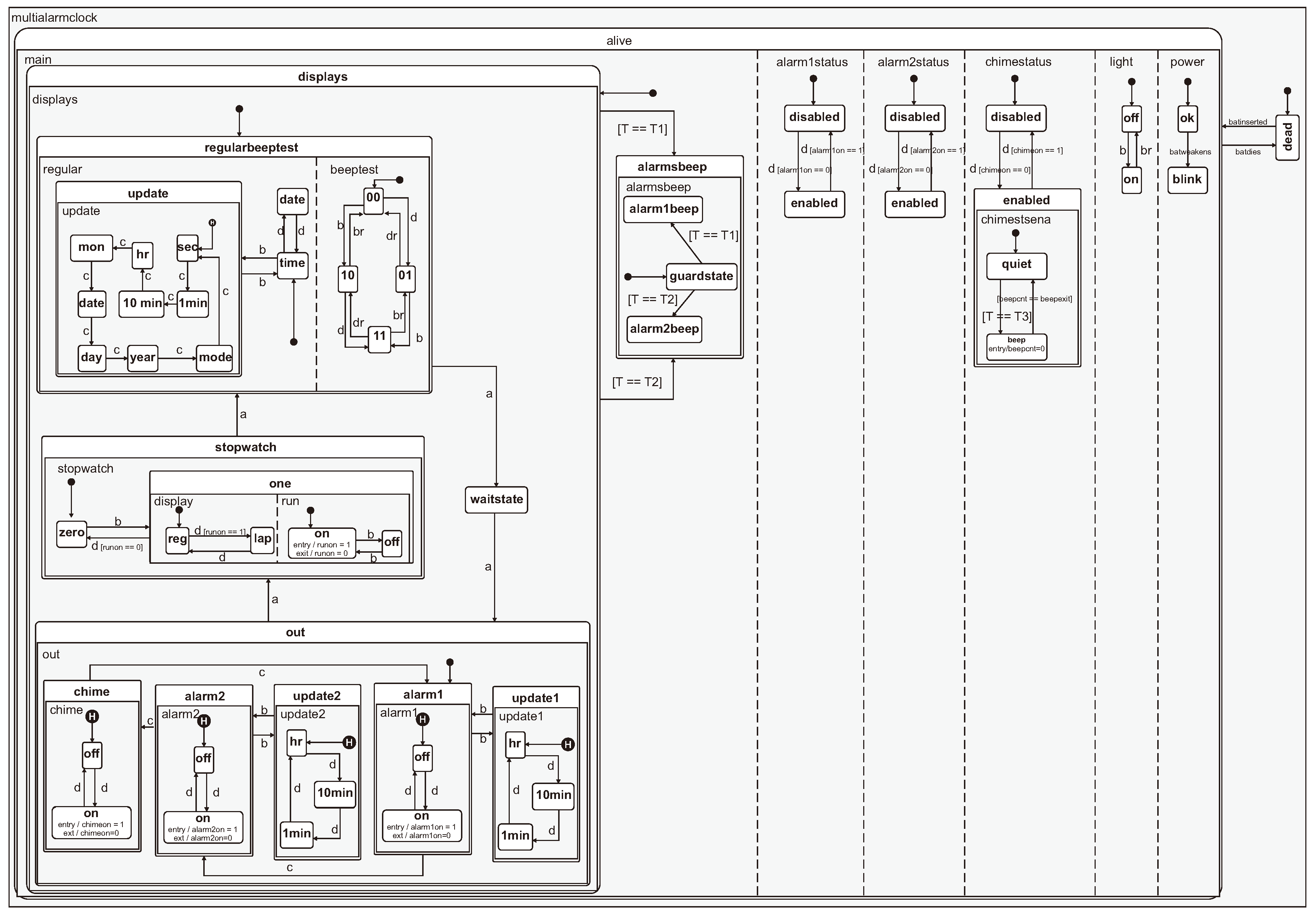
A recreation of the original Harel’s diagram is presented in
Figure 8. From it, alarm1-status, alarm2-status, and dead have been later removed as they have been found to be redundant with other states and the reset signal of the circuit. All the other aspects have been implemented, except deep history. In the hand-coded version; however, deep history has been included without much effort.
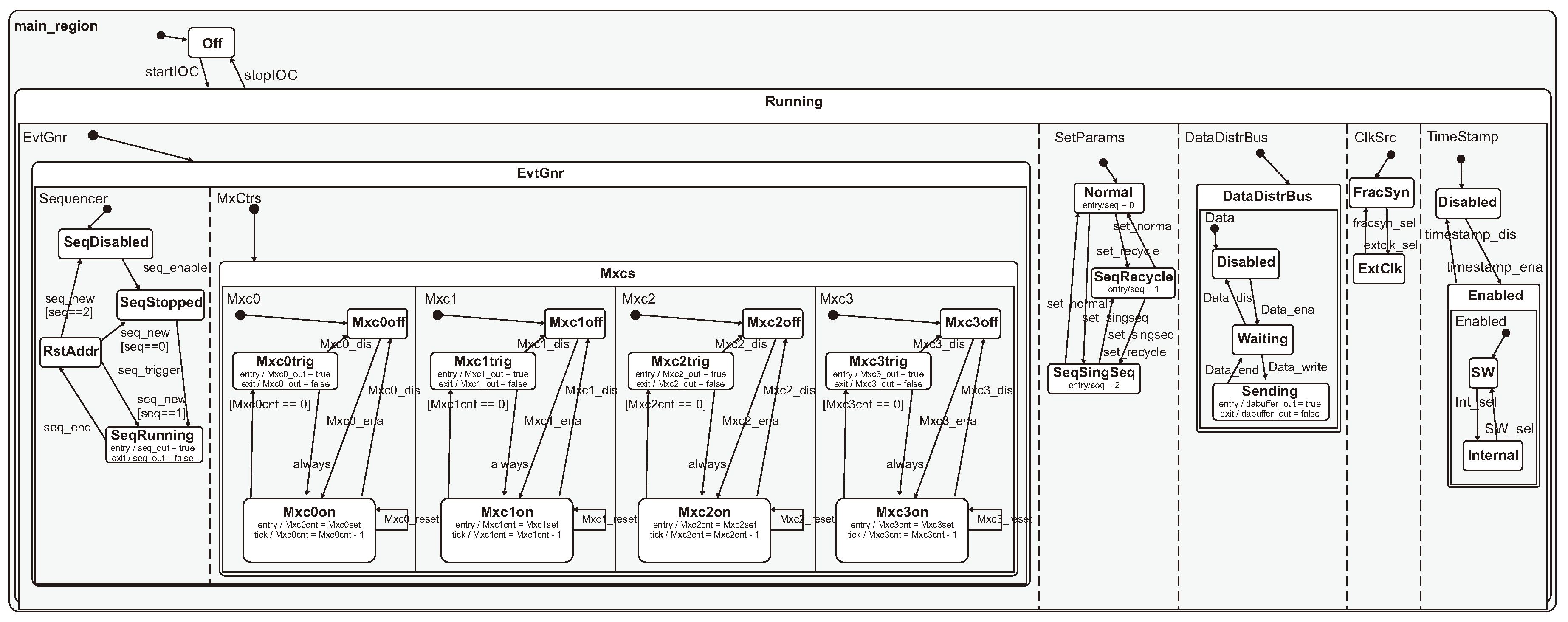
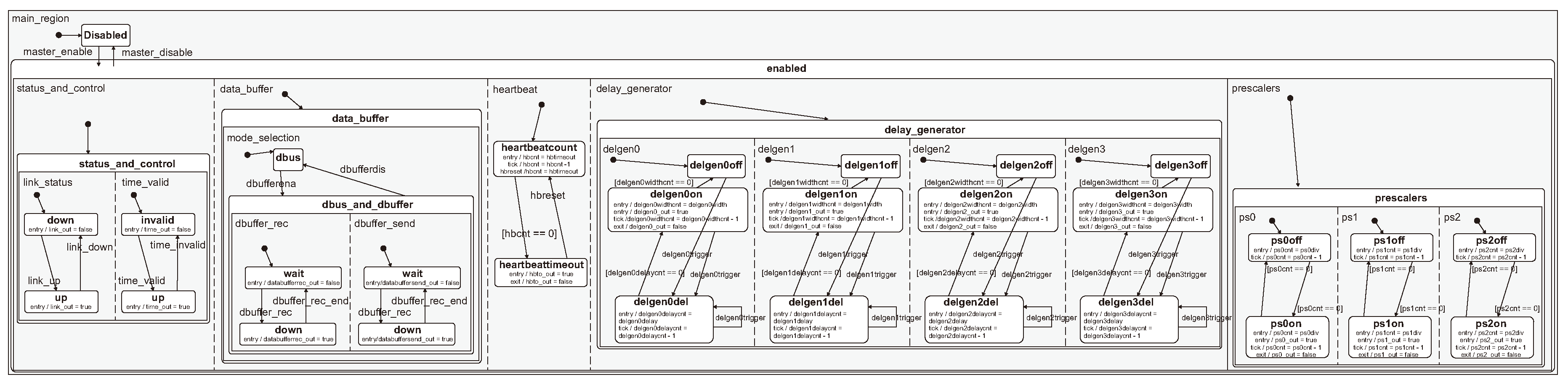
The EVG and EVR are shown in
Figure 9 and
Figure 10. Their structure is not as complex as that of the digital watch, apart from the fact that a significant number of AND superstates are required. In that sense, the digital watch tests the capability of correctly implementing most of the features of statecharts, while the remaining ones are used to compare the quality of the code in relation to the hand-written one.
These examples illustrate the main concepts of statecharts but they differ greatly in complexity. Harel’s watch, EVG and EVR specify a large number of AND-superstates, several inputs and conditions, but only Harel’s requires deeply nested hierarchy. We refer to the original papers [
4,
30].
Table 1 summarizes the main characteristics of the examples. Some of the figures have been expanded manually (between parentheses) in order to allow for some upgradability, which could extend the useful life of an embedded system.
The implementation of the example from
Figure 1 will be analysed first using the data from
Table 2. As it can be seen, the hand written code is more concise that any other option as: the automatic tool produces verbose code; and the microprogrammed architecture describes large multiplexers for condition and action selection (those 689 lines of VHDL code do not include the firmware). The number of logic blocks (Xilinx Kintex-7 look-up-tables) and flip-flops are similar for the hand-written and automatic implementations, but the microprogrammed architecture results in a large overhead. The latter architecture is the only one that requires RAM memories. Each microinstruction is 102 bits wide, requiring four 32-bit words. Thus, four double-port memories will support two AND-superstates. Then, twice that amount is needed to host up to four concurrent AND-superstates. Finally, the microprogrammed architecture is significantly slower than the hardwired ones, mainly due to the use of memory blocks and large multiplexers. This may have an impact on the performance of the systems or be irrelevant for a particular application. The difference in speed between the two hardwired circuits is not significant.
Table 3 shows results for Harel’s watch. As in the previous case, hand-written code is shorter and produces the smaller circuit. The automatic tool produces a similar circuit using a more verbose code. Again, the microprogrammed architecture is both significantly larger and slower than the other two architectures. In this case, each micro-instruction is 130-bit long, requiring five 32-bit words. Hence, five block of memory may host two AND-superstates, and four times that amount will host the planned eight concurrent AND-superstates.
The implementation results for EVG and EVR are similar and they are shown in
Table 4. As with the digital watch, the hand-coded implementations use slightly less resources than those generated by the tool. A quick inspection revealed that, in all three cases, the tool was using more flip-flops to encode the hierarchy of states, whereas the engineer decided to flatten the structure. As mentioned in
Section 3, superstates that only contain other superstates are not implemented. The microprogrammed implementations are similar to the digital watch, as the number of resources where expanded in the same way (see
Table 1). The differences are mainly attributed to the cost of managing a different number of AND superstates. Importantly, neither EVG nor EVR require deep-history. Harel’s watch does, but it may be implemented using simple history without losing usability.
Next, each strategy will be analysed comparing the implementation of the four statecharts. For the hardwired architectures, the number of lines of code and hardware components is proportional to the complexity of the statechart. The delay, however, does not increase significantly, as the critical path is defined by the most complex super-state, not the aggregation of many. This suggests that the synthesis of even larger statecharts should still produce fast circuits.
The circuits obtained using the automatic tool are comparable to those made by hand. A small resource overhead has been detected due to the implementation of some superstates. As hierarchy is more neatly implemented in the current way, we do not consider the need of rewriting the tool to optimize those cases. The main advantage of using our tool is the possibility of applying changes to the statechart in minutes and obtaining the HDL code in seconds. As a drawback, deep-history cannot be implemented.
The code size for the microprogrammed architectures is similar in all cases, as many of the components are the same even if they are instantiated in different amounts. The maximum differences are a factor 2.4 in logic blocks; and a factor 2.7 in flips-flops. In all cases the delay is very similar. The complexity of the microprogrammed architecture is largely due to the micro-instruction format, which is defined by the worst case. Particularly, state check in
Figure 1 requires evaluating five conditions. As a consequence, the architectures are not very different. A shorter format could have been chosen, as shown in
Figure 7, if some extra delay is acceptable. Eventually, the main difference is in the number of registers for reference values and the multiplexers that, as
Table 1 shows, are double the size in most cases. The delay in these architectures is mainly due to accessing the micro-memories and propagating the signals through large multiplexers. It can be seen that there is not a great increase, as the delay in multiplexers grows logarithmically with the number of inputs.
Any of the proposed examples can be implemented in any modern FPGA, with the exception of the smaller devices of some series. Furthermore, as cost does not grow exponentially with the complexity of the statechart, it is feasible to synthesize an extended architecture with extra inputs, counters, and outputs.
Although difficult to quantify, there are other advantages of using our tool and methodology in terms of ease and speed of support, maintainability and upgradability, which are compulsory in some cases, specifically in research facilities. The application that motivated our work presented in this paper, the ESS timing system, has some components that have a very flexible hardware, including FPGA Mezzanine Cards (FMCs), that require hardware reconfiguration. Some other timing system components are located in places where access is difficult or restricted, for example because the physical dimensions of the component location are tight or blocked, or because there may be radiation in the environment. In these cases it is important that the update process is fast and simple, since the time to perform it may be short (for example during a shutdown period of the facility) and it may be a technician without HDL experience performing the update, so using a visual tool such as statecharts to model the system is a big advantage. The new configuration should also be error-free, since the problems that could arise may be impossible to solve until the next shutdown or update period (in some cases planned for months in the future). They may even prevent the correct operation of some instruments, causing delays and extra costs in the experiments. In this kind of situations the work here presented is better and faster than the classical approach of writing by hand the hardware configuration of the systems. Our tool makes it easy and simple to update the hardware configuration even with no HDL programming experience, using a graphical approach and importing only one file to our tool. It also keeps the chance of errors as low as possible by automatically generating a correct VHDL file. Our methodology based on microprogramming allows updating and deploying configurations quickly without logic synthesis, since for the deployment only a new configuration is needed instead of a new bitfile. Furthermore, there is no dependency on the version of the synthesis software, so maintainability is easier. These characteristics are very important in some applications. Although the needs of ESS triggered the development of the work here presented, both the tool and methodology can be used for any other cases where the target system can be implemented as a statechart.
Each of these implementation options may produce circuits that are faithful to the original design in different degrees. Despite being time-consuming and error-prone, hand-written code has the potential to implement any characteristic of the statechart. The automatic tool and the micro-programmed architecture have the main limitation of not implementing deep-history. However, it is not expected that this produces malfunctioning problems. In the case of microprograms, it is possible that the architecture cannot evaluate complex conditions in a single cycle. In that case, evaluation is split in several cycles, and the resulting latency may be noticeable.


