End-to-End Noisy Speech Recognition Using Fourier and Hilbert Spectrum Features

Abstract

Despite the progress of deep neural networks over the last decade, the state-of-the-art speech recognizers in noisy environment conditions are still far from reaching satisfactory performance. Methods to improve noise robustness usually include adding components to the recognition system that often need optimization. For this reason, data augmentation of the input features derived from the Short-Time Fourier Transform (STFT) has become a popular approach. However, for many speech processing tasks, there is an evidence that the combination of STFT-based and Hilbert–Huang transform (HHT)-based features improves the overall performance. The Hilbert spectrum can be obtained using adaptive mode decomposition (AMD) techniques, which are noise-robust and suitable for non-linear and non-stationary signal analysis. In this study, we developed a DeepSpeech2-based recognition system by adding a combination of STFT and HHT spectrum-based features. We propose several ways to combine those features at different levels of the neural network. All evaluations were performed using the WSJ and CHiME-4 databases. Experimental results show that combining STFT and HHT spectra leads to a 5–7% relative improvement in noisy speech recognition.

1. Introduction

Recent advances in deep neural networks (DNNs) have significantly boosted the performance of automatic speech recognition (ASR) systems, which enables them to be applied in complex user applications such as voice-based web-search, intelligent personal assistants on mobile devices, etc. [1,2,3]. However, state-of-the-art speech recognizers are still far from reaching satisfactory robustness when facing challenging acoustical environments characterized by a high level of non-stationary noise.

Methods to improve noise robustness can be applied at various levels of an ASR system. Often, such methods are implemented prior to the feature extraction as an enhancement of the speech signal [4,5,6]. Methods working at the feature level may or may not be a part of the ASR system, as in the case of a deep denoising autoencoder [7,8,9]. Another approach is the joint training of the feature extractor and the acoustic model. This leads to performance improvements of both Gaussian mixture- [10] and neural network-based [11,12,13] acoustic models. Most of these strategies add components and additional hyper-parameters to the ASR system that require careful optimization.

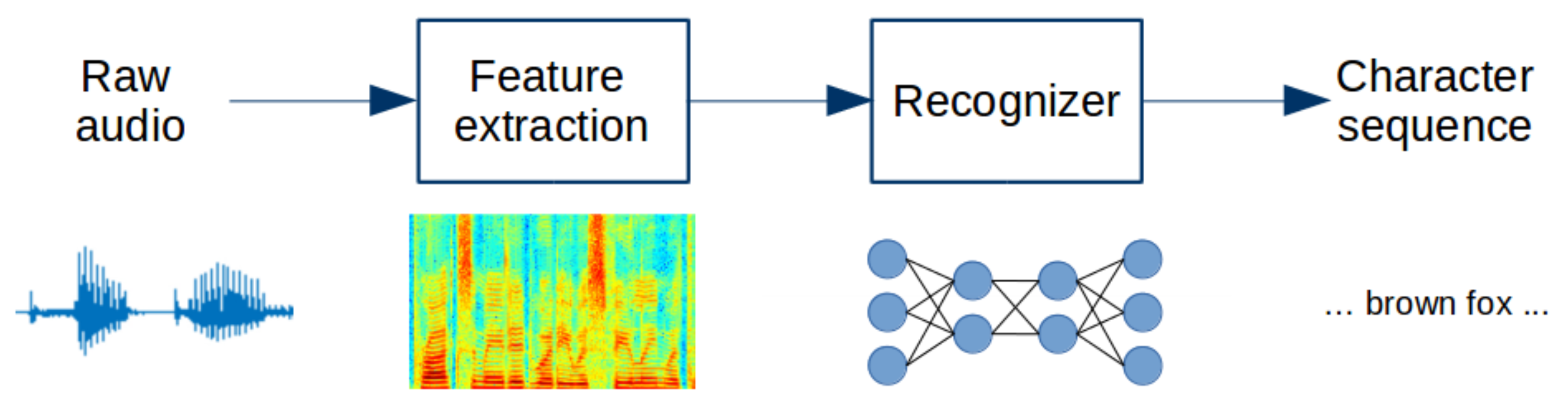
Nowadays, the dominant approach to building ASR systems is based on hybrid DNN-HMM systems consisting of a context-dependent acoustic model, pronunciation model, and n-gram language model. Training such systems is based on conditional independence assumptions and approximations [14]. In contrast to such hybrid systems, an end-to-end training approach facilitates the development of models without frame-level alignment and pronunciation modeling. As shown in Figure 1, this allows acoustic input features to be directly mapped to a character or phoneme sequences [15,16,17,18,19]. The most widely used and referred end-to-end techniques are connectionist temporal classification (CTC) [15], attention-based models [17], and recurrent neural network (RNN) transducer [16]. The main difference of the CTC is that it does not learn any context information during training, thus allowing only acoustic features to be evaluated [18].

Lately, noisy speech recognition research has been mostly concentrated on front-end speech enhancement or back-end DNN architecture and training objective functions, while less attention has been paid to the choice of input features. Short-Time Fourier Transform (STFT) spectrum features such as mel-frequency cepstral coefficients (MFCCs) [15] or log mel-filterbank spectrograms [16,18,20] are widely used. There have also been several attempts to train ASR systems with raw wave signals [19,21,22]. However, state-of-the-art end-to-end architectures still use STFT spectrum features. The STFT considers any signal to be piece-wise stationary and linear and treats it as a sum of predefined functions. A window function of a short speech frame is used to produce spectral characteristics of the signal. There is always a trade-off between the time and frequency resolution: i.e., increasing the frequency resolution decreases the temporal resolution. In contrast to STFT, the Hilbert–Huang Transform (HHT) method is suitable for non-stationary, non-linear signals and provides high time resolution in various frequency scales. The HHT method takes into consideration the signal frequency content as well as its variation.

In this work, we focus on neural network architectures that combine STFT- and HHT-based features in various ways. Our primary goal is to improve the ASR noise robustness without external pre-processing, such as speech enhancement, to the system. We propose several types of feature combinations at the input and intermediate levels of the ASR system. To the best of our knowledge, Hilbert spectrum features have not yet been used in an end-to-end DNN system.

To obtain the Hilbert spectrum, we use two methods: (1) Empirical Mode Decomposition (EMD) and (2) Variational Mode Decomposition (VMD). These methods are often applied in non-stationary signal processing and in some speech enhancement techniques. We built our ASR systems using the DeepSpeech2 architecture [23], which also serves as our baseline system. This DNN architecture consists of a convolutional layer stack and a recurrent layer stack. We apply our feature combination methods before the recurrent layer stack because, otherwise, separate recurrent layers for each feature channel would be required, and this will almost double the number of parameters, making the overall system difficult to train [24].

We propose several combination techniques that use the pattern representation capability of the convolutional neural network (CNN). Feature maps of the first few CNN layers tend to learn a variety of frequency and orientation patterns of the input [25]. We also look at more informative data representations by finding a correlation between the STFT and HHT feature channels and introduce an attention-based combination with different levels of detail.

All the ASR systems in this study were evaluated using WSJ and CHiME-4 databases. To obtain noise robustness estimates in a controlled scenario, we added natural noises to the recordings of the WSJ dataset. Partially overlapped sets of noises and signal-to-noise ratios (SNRs) were created for training, development, and testing. Speech recognition experiments demonstrated that combined feature models relied more on the STFT-based features when the speech signal was relatively clean, while HHT-based features acquired a higher combination weight when the SNR was below 10 dB. This achieved a 5–7% word error rate (WER) relative improvement over the STFT-based single-feature baseline. Finally, we evaluated our systems on the CHiME-4 one channel (1ch) track word recognition task, which contains real and simulated noisy data. The results obtained in this case showed a similar trend to that observed with the corrupted WSJ dataset. The relative WER improvement was 7% using the real noise test set. In all proposed models, the increase in the network parameter number is negligible with respect to the single-feature model. This demonstrates that HHT-based features can improve the end-to-end system noise robustness at a small additional cost.

2. Related Work

Combining various features to improve system performance and robustness is also a popular approach in some other speech processing tasks, such as speaker verification [26], emotion recognition [27], and speaker identification [28].

In some studies, the Hilbert spectrum has been used during conventional mel-frequency cepstral coefficient (MFCC) computations. In [29], HHT was used to obtain mel Hilbert frequency cepstral coefficients (MHFCCs) in a standard HMM-GMM ASR system. Here, the STFT step of MFCC computation was substituted with the calculation of the Hilbert spectrum by the EMD method. This improved the system accuracy by 4.4% relative to the STFT baseline. In [30,31], the Hilbert spectrum was used instead of the DCT step of the MFCC algorithm. In both cases, STFT and HHT features were evaluated for the digit recognition task and showed improved system performance in both clean and noisy conditions.

Adaptive mode decomposition techniques, such as EMD and VMD, are most often applied in speech enhancement tasks [4,32,33,34]. In [32], variational mode decomposition was used for spectral smoothing after the STFT step of the MFCC algorithm. The spectrum was smoothed over the frequency dimension. Higher-order modes obtained by VMD per frame were discarded, and then the smoothed spectrum was reconstructed using the first two modes only. In the clean training/testing conditions, VMD-MFCC yielded performance comparable to that of conventional MFCC. In mismatched conditions, in which clean data were used for training and the test set was corrupted by additive noise with SNRs of 10 and 15 dB, usage of the VMD-MFCC features allowed the overall performance to be improved by 13.3% relative to the baseline.

3. Feature Extraction

The Hilbert–Huang Transform (HHT) is a method of representing the signal in the time-frequency domain in terms of Intrinsic Mode Functions (IMFs) obtained by a mode decomposition method such as Empirical Mode Decomposition (EMD) or Variational Mode Decomposition (VMD).

3.1. Empirical Mode Decomposition

Empirical Mode Decomposition (EMD) is a method that decomposes the signal $x\left(n\right)$ into oscillatory components called intrinsic mode functions in a completely data-driven manner without the requirement of any a priori basis. Each IMF must satisfy two properties: (i) the number of extrema and the number of zero-crossings must either be equal to each other or differ by one; (ii) the mean value of the envelope defined by the local maxima and the envelope defined by the local minima is zero. The process of “sifting” employed to extract all the IMFs includes the following steps [35]:

• Calculate the upper- and lower-envelope of the signal $x\left(n\right)$ as well as their mean value ${\mu }_i$.
• Subtract the mean value from the data $h_i\left(n\right)=x\left(n\right)-{\mu }_i$, and use $h_i\left(n\right)$ going forward instead of $x\left(n\right)$.
• Repeat the first two steps until $h_i\left(n\right)$ satisfies the IMF properties. Then, it can be taken as an IMF component $c_i\left(n\right)=h_i\left(n\right)$.

Next, the IMF is subtracted from the signal to obtain the residue $r_i\left(n\right)=r_{i-1}\left(n\right)-c_i\left(n\right)$, where $r_0=x\left(n\right)$. This process should be repeated I times (total number of IMFs) until the last residue becomes a monotonic function. Then, the signal $x\left(n\right)$ can be expressed as

$$x\left(n\right)=r_I\left(n\right)+\sum _{i=1}^I{c}_i\left(n\right)$$

(1)

Although EMD is well known and widely used, it also has its share of limitations. A major drawback is mode-mixing. This is a phenomenon defined by the presence of disparate frequency scales within a single IMF and/or the presence of the same frequency scale in multiple IMFs.

To overcome this flaw, the authors of a previous study proposed performing EMD over an ensemble of signal and white noise [36]. The method is called Ensemble Empirical Mode Decomposition (EEMD). The addition of finite-amplitude white noise increases the number of extrema present in the inner residue signal $h_i\left(n\right)$. This leads to better estimates of the upper- and lower-envelopes of the signal when used as interpolation points in the sifting iteration. The EEMD process includes the following steps:

• Obtain L noisy copies of the signal $x\left(n\right)$ by adding L independent realizations of finite-amplitude normally distributed white noise: $x^l\left(n\right)=x\left(n\right)+\beta w^l\left(n\right)$, where $\beta$ is the signal-to-noise level of the added noise.
• Decompose each noise copy using EMD into a set of IMFs.
• Obtain the final IMF components as an ensemble average of the decompositions computed in the previous step.

It is expected that with an increasing number of white noise realizations L, the effect of noise will cancel out. However, there is no guarantee that the reconstructed signal will not include some residual white noise.

The EEMD method was further improved to Complementary Ensemble Empirical Mode Decomposition (CEEMD) [37]. It was observed that using white noise in pairs of opposite polarities substantially reduced the added noise effect.

The number of IMFs, maximum number of sifts, added noise level, and number of ensembles are the hyper-parameters in the EMD method. There are some recommendations for default values, such as 10 sifts and around 100 EMDs in an ensemble, but, in general, it is recommended to fine-tune these parameters on some small data subset.

To measure the quality of the obtained IMFs, the use of the orthogonality index (OI) between all IMFs has been proposed [35]. The decomposed modes should all be locally orthogonal to each other. The OI is defined as follows:

$$OI=\sum _{n=0}^N\left(\sum _{j=1}^{n+1}\sum _{k=1}^{n+1}{c}_j\left(n\right)c_k\left(n\right)/x^2\left(n\right)\right)$$

(2)

Ideally, a set of perfect orthogonal IMF components will give a value of zero for the OI. In practice, an OI smaller than 0.1 is assumed to be acceptable for speech signal decomposition [38].

3.2. Variational Mode Decomposition

The Variational Mode Decomposition (VMD) is an entirely non-recursive adaptive mode decomposition method [39]. It leads to a decomposition of the signal $x\left(n\right)$ into a predefined number of principal modes $c_i\left(n\right)$. It determines the relevant frequency bands adaptively and estimates the corresponding modes concurrently, thus properly balancing errors between them. The main advantages of this method are the theoretical rationale and robustness to noise and sampling.

Each mode $c_i\left(n\right)$ is mostly compact around the central frequency ${\omega }_i$. To assess the bandwidth of a mode, an analytic signal associated with each mode is computed by means of the Hilbert transform to obtain a unilateral frequency spectrum. Then, the frequency spectrum of each mode is shifted to baseband by multiplying it with an exponential tuned to the respective estimated central frequency. Finally, the bandwidth is estimated through the squared $l_2$ norm of the gradient. The resulting constrained variational optimization problem is defined as

$$\begin{array}{cc}\hfill \underset{\left\{c_i\left(n\right)\right\},\left\{{\omega }_i\right\}}{min}\{\sum _i& \parallel \frac{\partial }{\partial n}\left[\left(\delta \left(n\right)+\frac{j}{\pi n}\right)\ast c_i\left(n\right)\right]e^{-j{\omega }_{i}n}{\parallel }_2^2\},\hfill \\ \hfill & \mathrm{s}.\mathrm{t}.\sum _i{c}_i\left(n\right)=x\left(n\right)\hfill \end{array}$$

(3)

where $\left\{c_i\left(n\right)\right\}$ and $\left\{{\omega }_i\right\}$ are notations for the set of all modes and their center frequencies, respectively; $\delta (·)$ is the Dirac delta function, and * is the convolutional operator.

A possible way to render problem (3) as unconstrained is by using a quadratic penalty term and Lagrangian multipliers $\lambda$. The benefits of this combination are quick convergence and strict enforcement of the constraint. Therefore, the objective function becomes an augmented Lagrangian $\mathcal{L}$ as follows:

$$\begin{array}{cc}\hfill \mathcal{L}& (\left\{c_i\left(n\right)\right\},\left\{{\omega }_i\right\},\lambda ):=\hfill \\ & \alpha \sum _i\parallel \frac{\partial }{\partial n}\left[\left(\delta \left(n\right)+\frac{j}{\pi n}\right)\ast c_i\left(n\right)\right]e^{-j{\omega }_{i}n}{\parallel }_2^2+\hfill \\ & \parallel x\left(n\right)-\sum _i{c}_i\left(n\right){\parallel }_2^2+〈\lambda \left(n\right),x\left(n\right)-\sum _i{c}_i\left(n\right)〉,\hfill \end{array}$$

(4)

where $\alpha$ is the quadratic penalty weight, and $\langle ·,·\rangle$ corresponds to the inner product.

The solution to the original minimization problem (3) can now be found as the saddle point of the objective function (4) in a sequence of iterative sub-optimization called the alternate direction method of multipliers [40].

After optimization, the resultant modes $\left\{{\widehat{c}}_i\right\}$ in the frequency domain can be calculated as

$${\widehat{c}}_i\left(\omega \right)=\frac{\widehat{x}\left(\omega \right)-{\sum }_{k\ne i}{\widehat{c}}_k\left(\omega \right)+\frac{1}{2}\widehat{\lambda }\left(\omega \right)}{1+2\alpha {(\omega -{\omega }_i)}^2}$$

(5)

where ${\widehat{c}}_i\left(\omega \right),\widehat{x}\left(\omega \right),\widehat{\lambda }\left(\omega \right)$ are the frequency domain representations of $c_i\left(n\right),x\left(n\right),\lambda \left(n\right)$, respectively. Similarly, center frequencies ${\omega }_i$ can be updated as

$${\omega }_i=\frac{{\int }_0^{\infty }\omega {\left|{\widehat{c}}_i\left(\omega \right)\right|}^{2}d\omega }{{\int }_0^{\infty }{\left|{\widehat{c}}_i\left(\omega \right)\right|}^{2}d\omega }$$

(6)

The complete optimization of VMD can now be summarized as follows:

• Initialize the set of modes $\left\{{\widehat{c}}_i^1\left(n\right)\right\}$, set of central frequencies $\left\{{\omega }_i^1\right\}$, set of Lagrangian multipliers $\left\{{\widehat{\lambda }}^1\left(n\right)\right\}$, and iteration counter $m=0$.
• Increment the iteration counter $m=m+1$.
• Update each mode in the set $\left\{c_i\left(n\right)\right\}$ and its associated center frequency $\left\{{\omega }_i\right\}$ for all $\omega >0$ as follows:

  $$\begin{array}{cc}\hfill {\widehat{c}}_i^{m+1}\left(\omega \right)=& \frac{\widehat{x}\left(\omega \right)-{\sum }_{k<i}{\widehat{c}}_k^{m+1}\left(\omega \right)}{1+2\alpha {(\omega -{\omega }_i^m)}^2}-\hfill \end{array}$$

  $$\begin{array}{c}\frac{{\sum }_{k>i}{\widehat{c}}_k^m\left(\omega \right)+\frac{1}{2}{\widehat{\lambda }}^m\left(\omega \right)}{1+2\alpha {(\omega -{\omega }_i^m)}^2}\hfill \end{array}$$

  (7)

  $$\begin{array}{cc}\hfill {\omega }_i^{m+1}=& \frac{{\int }_0^{\infty }\omega {\left|{\widehat{c}}_i^{m+1}\left(\omega \right)\right|}^{2}d\omega }{{\int }_0^{\infty }{\left|{\widehat{c}}_i^{m+1}\left(\omega \right)\right|}^{2}d\omega }\hfill \end{array}$$

  (8)
• Update Lagrangian multipliers $\lambda \left(n\right)$ for all $\omega >0$ as follows:

  $${\widehat{\lambda }}^{m+1}\left(\omega \right)={\widehat{\lambda }}^m\left(\omega \right)+\tau \left[\widehat{x}\left(\omega \right)-\sum _i{\widehat{c}}_i^{m+1}\left(\omega \right)\right]$$

  (9)

  where $\tau$ is an update parameter for the Lagrangian multipliers.
• Check for convergence:

  $$\sum _i\frac{\parallel {\widehat{c}}_i^{m+1}\left(n\right)-{\widehat{c}}_i^m{\parallel }_2^2}{\parallel {\widehat{c}}_i^m{\parallel }_2^2}<ϵ$$

  (10)
  If this condition is met, terminate decomposition and set $\left\{c_i\left(n\right)\right\}=\left\{{\widehat{c}}_i^{m+1}\left(n\right)\right\}$, $\left\{{\omega }_i\right\}=\left\{{\omega }_i^{m+1}\right\}$. Otherwise, return to step 2.

The number of modes i, weight of the quadratic penalty term $\alpha$, update parameter for the Lagrangian multipliers $\tau$, and convergence condition $ϵ$ are the hyper-parameters of the VMD algorithm. They should be fine-tuned on some small dataset.

To evaluate the quality of the obtained IMFs, we used the OI, Equation (2), the same as for the EMD. Since there is no guarantee that the signal will be decomposed fully in the chosen number of modes, we also calculate the residual error as follows:

$$RE=\sum _n\frac{x\left(n\right)-{\sum }_i{c}_i\left(n\right)}{x\left(n\right)}$$

(11)

The optimal choice of parameters can be found by minimizing both the orthogonality index and residual error together.

3.3. Hilbert Spectrum

The IMFs derived from the signal are represented in terms of their instantaneous amplitude envelopes and frequencies by the Hilbert transform [26]:

$$c_i\left(n\right)\stackrel{\mathrm{Hilbert}\mathrm{transform}}{\to }{a}_i\left(n\right)e^{j{\theta }_i\left(n\right)},f_i\left(n\right)=\frac{1}{2\pi }\frac{d}{dt}{\theta }_i\left(n\right),$$

(12)

where $a_i\left(n\right)$, ${\theta }_i\left(n\right)$, and $f_i\left(n\right)$ represent the instantaneous envelope, phase, and frequency of $c_i\left(n\right)$.

The Hilbert spectrum $H(k,n)$ (HS) is the distribution of the signal energy as a function of time and frequency. The number of desired frequency bins k is a hyper-parameter of the HS:

$$H(k,n)=\sum _{i-1}^I{a}_i\left(n\right)w_i^{\left(k\right)}\left(n\right),$$

(13)

where $w_i^{\left(k\right)}$ is a weight factor that is 1 if $f_i\left(n\right)$ falls within the kth band and is 0 otherwise.

4. System Description

In this section, we describe a neural network architecture which represents the recognizer part of the end-to-end speech recognition system shown in Figure 1. As a baseline DNN we adopted the DeepSpeech2 model [23] which consists of CNN and RNN stacks illustrated in Figure 2. It was used for single-feature models as well as a basis for the proposed feature combination methods. Within this model, there are several possible locations to combine features:

• At the input level: before the CNN stack;
• At the intermediate level: between the CNN and RNN stacks;
• At the top level: between the RNN stack and the final dense layer.

We start from straightforward ‘naive’ combinations at the input and intermediate levels. Then, we describe attention-based combinations at the intermediate level. Combinations at the top level will introduce a large number of additional training parameters due to the doubling of the RNN stack. Since it is difficult to compare systems with big differences in the parameter number [24], in this paper, we do not consider combinations at the top layer.

4.1. Single Feature System

The DeepSpeech2 model architecture [23] we used for our single-feature models is shown in Figure 2. It takes a spectrogram as input followed by two CNN layers and a number of recurrent layers topped with one dense layer. Batch normalization is applied after each CNN layer and before every recurrent and dense layer starting from the second recurrent layer.

We assume that both STFT and HHT spectra are already extracted from the speech signal and presented as 3D feature matrices suitable for 2D CNNs. These dimensions are the number of channels (one channel in the case of a single feature), the number of frequency bins, and the number of time bins, while in a conventional image-based 2D CNN, these dimensions are the number of channels (one for a gray-scale image or three for RGB colors), image height, and image width.

4.2. Naive Feature Combination

Here, we consider three types of feature combinations while keeping the general architecture of the single-feature system. First, we combine them on the input level. Both spectra are concatenated along the channel dimension so that the first channel is the STFT spectrogram and the second channel is the HHT spectrogram, as shown in Figure 3a. We refer to this system as “2ch CNN”. Second, we train different CNN stacks for each feature type and then concatenate flattened feature maps before feeding them to the recurrent stack, as shown in Figure 3b. We call this system “ConcatCNN”. Although it is possible to add or multiply these feature maps instead of concatenating them, preliminary experiments showed that the concatenation resulted in better model performance.

Another more intelligent way to combine the CNN feature maps is to use the correlation between them. In [41], a correlation layer was introduced to predict optical flow from two input images. The concatenation operation can be replaced with correlation, as shown in Figure 3b. It performs multiplicative patch comparisons between two multi-channel feature maps, ${\mathbf{f}}_1$ and ${\mathbf{f}}_2$. The ‘correlation step’ of two patches centered at ${\mathbf{x}}_1$ in the first map and ${\mathbf{x}}_2$ in the second map is defined as

$$c({\mathbf{x}}_1,{\mathbf{x}}_2)=\sum _{\mathbf{o}\in [-k,k]\times [-k,k]}\langle {\mathbf{f}}_1({\mathbf{x}}_1+\mathbf{o}),{\mathbf{f}}_2({\mathbf{x}}_2+\mathbf{o})\rangle$$

(14)

for a square patch of size K: = 2k + 1. This step is identical to one step of convolution in neural networks, but instead of convolving the input with a filter, it convolves one input with the other input. Thus, the correlation layer does not add trainable parameters to the network.

For computational reasons, patch combinations can be limited by the maximum correlation displacement. Given a maximum displacement d for each location ${\mathbf{x}}_1$, correlations $c({\mathbf{x}}_1,{\mathbf{x}}_2)$ are computed only in a neighborhood of size D: = 2d+1 by limiting the range of ${\mathbf{x}}_2$. Since these relative displacements are organized in channels, the output size is $(w\times h\times (D^2+2d+1))$, where w and h are the width and height of the feature maps.

To return to the same number of channels as that used in other network combinations, we added one more convolution layer with a [1 × 1] kernel to make the number of output channels the same as that in the second convolution layer. This type of system is denoted as “CorrCNN”.

4.3. Attention-Based Feature Combinations

4.3.1. Attentive Vector/Scalar Combination

In [42], the authors proposed fusing several modalities with an attention-based layer. This improved the video description system’s ability to dynamically determine the relevance of each modality to different parts of the description. To calculate the attentive weights of each modality, they used the CNN output of the encoder and the temporal attention states of the decoder. Finally, single scalar weights were applied to each modality. Our attentive combination differs from this multimodal fusion in the attention weight calculation. As depicted in Figure 4a, we first reshape CNN outputs by flattening the height and channel dimensions while keeping the time dimension as it is. Then, we calculate the attentive combination of the reshaped CNN outputs as

$${\mathcal{F}}_{Comb}={\beta }_{STFT}{\mathcal{F}}_{STFT}+{\beta }_{HHT}{\mathcal{F}}_{HHT}$$

(15)

where ${\beta }_{STFT}$ and ${\beta }_{HHT}$ are attention weights obtained as follows:

$${\beta }_l=\frac{exp\left(v_l\right)}{{\sum }_{k}exp\left(v_k\right)},$$

(16)

where k is the number of features (i.e., in our case, k = 2), $l\in \{STFT,HHT\}$, and v is a feature projection. We consider two variants of this projection:

(1)

$v_l$ is calculated as an element-wise attention weight vector:

$$v_l=tanh(W_{B,l}{\mathcal{F}}_l+b_{B,l}),$$

(17)

where $W_{B,l}$ is a projection matrix and $b_{B,l}$ is a bias vector.

(2)

$v_l$ is calculated as a scalar attention weight, similar to [42]:

$$v_l=w_B^{T}tanh(W_{B,l}{\mathcal{F}}_l+b_{B,l}),$$

(18)

where $w_B$ is a vector, and the resulting $v_l$ is a scalar.

The difference is that the importance of attention weights is more detailed in case (1) and less detailed in case (2). We refer to the system using the attention vector as “AV-CNN” and the system with scalar attention as “AS-CNN”.

4.3.2. Squeezed Attentive Combination

Both the attention vector and scalar combinations use reshaped CNN output, possibly losing some pattern representation learned by the CNN channels in the stack. In [43], the squeeze-and-excitation block was proposed to improve the representation quality produced by the CNN network by explicitly modeling interdependencies between the channels of its convolutional features. This block allows the network to utilize global information to selectively emphasize informative convolutional feature maps. We adapted this global channel information to combine CNN outputs with squeezed attention. As can be seen in Figure 3b, we use squeezed channel-wise CNN outputs to obtain the attention weights of both CNN outputs.

First, we obtain channel-wise statistics $z_{c,l}\in R^C$ using global average pooling applied to the CNN output $U_l\in R^{HxWxC}$:

$$z_{c,l}=\frac{1}{H+W}\sum _{i=1}^H\sum _{j=1}^W{u}_{c,l}(i,j),$$

(19)

where $l\in \{STFT,HHT\}$.

The obtained vector $Z_l=\left\{z_{c,l}\right\}$ is used to calculate scales $S_l=\left\{s_{c,l}\right\}$ for each channel. This operation aims to fully capture channel-wise dependencies and dynamical change in the interaction between channels. We employ a simple gating mechanism, which consists of two feed-forward layers:

$$S_l=\sigma (W_{2,l}\ast \delta (W_{1,l}\ast Z_l))$$

(20)

where $\delta$ is a ReLU activation function and $\sigma$ is a sigmoid activation function. The size of the inner layer can be optimized per input. Plugging these scales from both outputs into Equation (16), we can obtain weights for each channel:

$${\beta }_{c,l}=\frac{exp\left(s_{c,l}\right)}{{\sum }_{k}exp\left(s_{c,k}\right)},$$

(21)

where k is the number of features (i.e., in our case, k = 2). In the final combination, each channel of each CNN output is scaled with the obtained weights.

$$\begin{array}{cc}\hfill {\mathcal{F}}_{comb}& ={\mathcal{F}}_{STFT}+{\mathcal{F}}_{HHT},\hfill \end{array}$$

(22)

$$\begin{array}{cc}\hfill f_{c,l}& =u_{c,l}\ast {\beta }_{c,l},\hfill \end{array}$$

(23)

where ${\mathcal{F}}_l=\left\{f_{c,l}\right\}$.

By squeezing global spatial information into a channel descriptor z, we can explicitly model channel interdependencies. Calculating the weights of each spectrum allows us to increase the network sensitivity to the most important features. This squeezed attention combination system is called “SA-CNN”.

5. Experimental Setup

5.1. Data Description

The first set of experiments was conducted on the WSJ dataset. As training data, we used the SI-284 part, which consisted of about 37K utterances (81.2 h). Evaluation was carried out on the “eval92” test set of 333 utterances (0.7 h), and the hyper-parameter selection and early stopping were performed on the “dev93” development set, which had 503 utterances (1.1 h). There were a total of 28 character labels: 26 letters, space, and a ‘blank’ symbol. To obtain noise robustness estimates in a controlled scenario, we performed data augmentation and used multi-condition training to build all of the models. All splits of the dataset were corrupted with noises from the Aurora 2 corpus [44] at various SNR levels. To simulate unseen acoustic conditions, we used different but overlapping sets of noise types and SNR levels. These conditions are summarized for each split in

Table 1. Augmented datasets obtained from the WSJ corpus. Conditions, which are different between training and test sets, are highlighted with italic font.

	Training Set	Mixed Dev	Noisy Test A	Noisy Test B
Noise type	airport, babble,	babble, restaurant,	babble, restaurant,	train
	restaurant, street	street	street
SNR	5 dB, 10 dB, 20 dB	5 dB, 10 dB, 20 dB	0 dB, 5 dB,	0 dB, 5 dB,
			10 dB, 20 dB	10 dB, 20 dB

. Each utterance in the development set was either corrupted with one of the noise conditions or kept clean with equal probability. We refer to this set as Mixed Dev. We grouped the known noise data types, such as ‘babble’, ‘restaurant’, and ‘street’, into Noisy Test A, and the unseen noise data type ‘train’ was put in Noisy Test B. Since noise signals have much larger lengths than speech recordings, a noise segment of the desired length was cut out of the whole noise recording with a randomly selected starting point. To add noise at a certain SNR, the speech signal level was calculated for the active speech segments only, ignoring silent segments in the beginning and the end of the recording as well as the long pauses between the words.

For the language model integration, we used an extended 3-gram language model (LM) as produced by Kaldi s5 recipe [45]. Its vocabulary size was 146K words, while the standard WSJ vocabulary size was 5K words.

In the final set of experiments, we used the CHiME-4 1ch word recognition task [46]. The CHiME-4 challenge was designed to be close to a real-world scenario. Training data (33 h) consisted of three parts: 7138 clean utterances, 1600 real noise utterances, and 7138 simulated noise utterances. The clean part was the SI-84 part of the WSJ dataset. The ‘real’ speech part was recorded using a tablet device with an array of six microphones in everyday environments: cafe, street junction, public transport, and pedestrian area. The same transcripts as those in the clean part were used for these recordings. To create the simulated part, the original WSJ SI-84 clean data were corrupted with noise collected in the same environments as the ‘real’ part. The development set consisted of real and simulated parts, each containing 1640 utterances (∼5.6 h). We used this set to optimize the hyper-parameters and perform early stopping. The test set also consisted of real and simulated parts, each consisting of 1320 utterances (∼4.4 h). We used 1ch (one channel) track lists of the development and test sets.

We augmented the real and simulated parts of the CHiME-4 training set with speech utterances from channels 3, 4, 5, and 6. Recordings from channel 2 were excluded since the second microphone is located on the back of the tablet. The actual SNRs of the data are not provided for any part of the dataset.

For the language model integration, we used a 5-gram language model with a 5K vocabulary size. This model is standard for this dataset.

5.2. Model Hyper-Parameters

In the convolution layer stack, we used two layers with stride 2 along the time dimension in the first layer. We performed an extensive search of optimal kernel sizes for both layers using STFT- and HHT-based models for the same input dimensionality. We started with [41 × 11], [21 × 11], which were used in previous works [23,47], gradually reducing kernel sizes along both dimensions. We found that reducing kernels to [5 × 3] constantly resulted in better performance for all models. The usage of pooling layers or stride over the frequency dimension was optimized per model on the development set.

For models trained on the WSJ and CHiME-4 datasets, the recurrent layer stack consisted of six layers with 768 BiGRU units. The approximate number of trainable parameters per model is summarized in

Table 2. Approximate number of trainable parameters per model.

Model	Number of Parameters
Single feature model	44.4 M
Two channels combination (2ch CNN)	44.4 M
Concatenated CNNs (ConcatCNN)	50.2 M
Correlated CNNs (CorrCNN)	44.6 M
Attentive vector combination (AV-CNN)	47.6 M
Attentive scalar combination (AS-CNN)	47.6 M
Squeezed attention combination (SA-CNN)	44.6 M

.

All our models were trained using the CTC objective function and stochastic gradient descent (SGD) optimizer. For the models trained on WSJ data, we initialized the learning rate to 0.003 and multiplied it by 0.97 after every epoch. Every model was trained until the WER, obtained on the development set, stopped decreasing over 10 consecutive epochs or for a maximum of 80 epochs. For the models trained on CHiME-4 data, we used the same learning rate and decay schedule, but the maximum number of epochs was 55. For experiments with both datasets, the maximum number of epochs was chosen empirically using the baseline model.

At the test time, character sequences were obtained with simple best path decoding to calculate the character error rate (CER). To obtain the word error rate (WER) with language model rescoring, we used beam search and optimized the language model score separately for each experiment.

5.3. Training Schedule and Strategy

For the WSJ dataset, we used multi-condition training, a widely used technique to improve the noise robustness of a speech recognition model. In our experiments, we adopted the curriculum learning method described in [48] called accordion annealing (ACCAN). Since we used more than one noise type and a larger amount of training data, we introduced a few changes into ACCAN. We started training with clean data only for 10 epochs. Then, we started to add noisy data with the lowest SNR level with a probability of 0.05. We increased this probability by 0.05 every K epochs and added the next SNR condition in increasing order after $S_1$ and $S_2$ epochs. The optimal number of epochs K and $S_i$ were identified using single-feature models trained with STFT- or HHT-based features. We tried about 10 training schedules for each model, and the most accurate ones were obtained when K = 2, $S_1$ = 20, and $S_2$ = 40. We trained our combined-feature models and the single-feature models using the same schedule.

Since recordings of the CHiME-4 dataset had noisy utterances with undefined SNRs, we used two stages for training. First, we trained using clean data only for 10 epochs. Then, we added all augmented data from the real and simulated parts and trained until convergence or when the maximum number of epochs was reached.

5.4. Feature Extraction

All STFT spectrograms were obtained using a 20 ms window length and 10 ms shift. Considering the standard WSJ and CHiME-4 sampling rate of 16 kHz, we could get a maximum of 161 frequency bins per one time window. Thus, the size of the 3D input features was 1 for the channel, 161 for the number of frequency bins, and a variable number of time bins for each batch.

To obtain the EMD-HHT spectrum, we used the complementary ensemble empirical mode decomposition (CEEMD) [37] implemented in Matlab [49]. For each utterance, we obtained 100 ensembles of 16 IMFs with a maximum number of 10 sifts and noise level 2. As suggested in [35], we checked the quality of the obtained IMFs with the orthogonality index (OI) measure, which is recommended to be less than 0.1. If the OI was more than 0.1, we reduced the noise level and/or the maximum number of sifts and ran the process again.

To obtain the VMD-HHT spectrum, we used the Matlab library provided by the author of the method [39]. We found that the most sensitive parameter of the VMD method was the quadratic penalty weight $\alpha$. When $\alpha$ was changed from 500 to 22,000, the overage OI decreased linearly, while the average RE increased exponentially. Thus, we selected VMD hyper-parameters based on the average RE value. For a fair comparison, we kept the number of IMFs the same as that for the EMD method. The lowest RE value was obtained when $\alpha$ = 2500, $\tau$ = 0, and $ϵ$ = ${10}^{-7}$.

For all STFT, EMD-HHT, and VMD-HHT spectra, we kept the same time resolution, which meant that one time bin in the HHT spectrum represented a 10 ms window. To extract features for the training, clean test, and noisy test sets, we used the EMD and VMD hyper-parameters that were found to be the most suitable on the development set.

Both the WSJ and CHiME-4 datasets share the same acoustic units since the same set of transcriptions is used.

6. Experimental Results

In the following subsections, we describe the results of the experiments conducted to assess the noise robustness of the proposed feature combination methods.

6.1. WSJ Dataset

First, we trained separate STFT and HHT single-feature models using the data augmentation and curriculum learning techniques described in Section 5.3. Character and word error rates (CER, WER) obtained with single-feature models are presented in

Table 3. Character error rate (CER) and word error rate (WER) results (%) of clean and noisy tests for single-feature models trained on the WSJ dataset (The best results for each set are highlighted with bold font).

Feature	Clean Test		Noisy Test A		Noisy Test B		Average
	CER	WER	CER	WER	CER	WER	CER	WER
STFT	4.5	8.8	9.8	17.3	9.6	17.2	8.0	14.4
EMD-HHT	5.4	10.5	13.7	23.1	13.0	22.2	10.7	18.6
VMD-HHT	4.8	9.2	10.6	18.3	10.7	18.4	8.7	15.3

. Overall, neither of the HHT-based single-feature models outperformed the STFT-based one, which is consistent with the previous results on different speech tasks [26,27]. On the other hand, the VMD model was more accurate than the EMD model.

Next, we evaluated our combined feature models described in Section 4.2 and Section 4.3. We fine-tuned the hidden layer size of the SA-CNN model using the mixed development dataset. It was 32 nodes for the EMD-based feature combination and 128 nodes for the VMD-based one. Thus, the increase in the trainable parameters per model was negligible, as is shown in Table 2. The displacement parameter d of the correlation layer was also optimized over the development set. We found that smaller values of d ≈ 20–30% of the feature map height led to better performance. Here, we used d = 8.

The CER and WER results of the WSJ experiments are summarized in

Table 4. CER and WER results (%) of clean and noisy tests for all the models trained on the WSJ dataset. Noisy Test A has the same noise types as the training set. Noisy Test B has a noise type that is not used during training (The best results for each set are highlighted with bold font).

Feature	Model	Clean Test		Noisy Test A		Noisy Test B		Average
		CER	WER	CER	WER	CER	WER	CER	WER
STFT	Baseline	4.5	8.8	9.8	17.3	9.6	17.2	8.0	14.4
EMD-HHT	2ch CNN	4.5	8.7	9.3	16.5	8.9	15.9	7.6	13.7
	ConcatCNN	4.6	8.6	9.8	17.2	9.4	16.9	7.9	14.2
	CorrCNN	5.0	9.5	10.5	18.8	10.5	18.7	8.7	15.6
	AV-CNN	4.6	8.5	9.8	16.9	9.6	16.7	8.0	14.1
	AS-CNN	4.7	8.6	10.1	17.2	9.9	17.0	8.2	14.2
	SA-CNN	4.6	8.5	9.7	16.6	9.4	16.5	7.9	13.9
VMD-HHT	2ch CNN	4.4	8.4	9.7	16.8	9.4	16.4	7.8	13.9
	ConcatCNN	4.3	8.4	9.7	17.0	9.4	16.8	7.8	14.1
	CorrCNN	4.8	9.1	10.8	19.0	10.6	18.3	8.8	15.5
	AV-CNN	4.6	8.5	10.0	17.4	9.8	17.2	8.1	14.4
	AS-CNN	4.8	8.8	10.1	17.4	10.1	17.6	8.3	14.6
	SA-CNN	4.3	8.0	9.3	16.3	9.2	16.2	7.6	13.5

. The majority of models trained with EMD- and VMD-based features outperformed the STFT baseline. The only exception here was the CorrCNN model. We suppose that STFT and HHT spectra were too different to gain any advantage from their correlation. Analyzing the attention combination performance, we see that squeezed attention (SA-CNN) outperformed both AV-CNN and AS-CNN, which we expected to some extent. The lowest WERs from the clean test and Noisy Test A sets were achieved using the SA-CNN combination of STFT- and VMD-based features. The lowest WER from the unseen Noisy Test B was achieved using the 2ch CNN EMD-based feature combination. All models generalized well to mismatched training-testing conditions, as no big drop in performance of either baseline or combined feature models was observed.

The best CER and WER results were obtained by the models in which feature combination was performed along the channel dimension at different levels of the model. As the performances of the 2ch CNN model using EMD-based features and SA-CNN model using VMD-features were very close for both noisy test sets, we examined performance for each noise type averaged over different SNRs and for each SNR averaged over the noise type. It was found out that the SA-CNN model outperformed 2ch CNN on the test set corrupted with the ‘street’ noise, which is a part of Noisy Test A. This noise was also the most difficult noise type for the recognition. The WER values of the baseline, 2ch CNN, and SA-CNN were 19.5%, 19.0%, and 18.0%, respectively. Otherwise, 2ch CNN showed better performance when SNR was 0 dB. The WER values of the baseline, 2ch CNN, and SA-CNN were 30.7%, 29.0%, and 29.5%, respectively. This suggests that SA-CNN was more advantageous when dealing with a challenging noise type, while 2ch CNN was more advantageous when dealing with low-SNR noisy conditions.

Finally, we performed statistical significance tests on the results obtained with the SA-CNN model trained with VMD-based features, 2ch CNN trained with EMD-based feature combinations, and the baseline model trained with STFT-based features. According to the Matched Pairs Sentence Segment Word Error Test (MPSSW) [50] between the SA-CNN and baseline models, all WER results on each test set were statistically significant with p-value < 0.05. MPSSW between 2ch CNN and baseline models showed that WER improvement was statistically significant with p-value < 0.05 when calculated for the noisy test sets results.

6.2. CHiME-4 Dataset

Up to this point, the experiments were performed in simulated noisy conditions only. Next, we investigated whether using additional HHT-based features could help in real noisy environments.

The CER and WER results obtained separately for simulated and real noisy test and development (dev) sets are summarized in

Table 5. CER and WER results (%) of clean and noisy tests for all the models trained on the CHiME-4 dataset (The best results for each set are highlighted with bold font).

Feature	Model	Simulated Dev		Real Dev		Simulated Test		Real Test
		CER	WER	CER	WER	CER	WER	CER	WER
STFT	Baseline	17.1	25.4	16.2	23.5	24.8	36.3	25.3	38.3
EMD-HHT	2ch CNN	16.4	23.6	15.4	22.0	24.5	35.5	24.6	36.5
	ConcatCNN	16.0	23.3	14.9	21.8	24.0	35.5	24.0	36.3
	CorrCNNs	17.3	25.6	16.2	23.9	25.0	37.3	25.6	39.4
	AV-CNN	16.2	23.5	14.6	21.1	23.8	34.6	23.7	35.6
	AS-CNN	16.1	23.6	14.8	21.8	23.8	35.3	24.4	36.8
	SA-CNN	16.1	23.3	14.3	20.8	23.8	34.5	23.8	35.6
VMD-HHT	2ch CNN	16.6	24.0	15.4	22.2	24.5	35.4	25.0	37.5
	ConcatCNN	16.3	23.8	15.0	21.7	24.1	35.3	24.3	36.6
	CorrCNN	17.4	26.3	16.0	24.0	24.9	37.0	25.3	38.9
	AV-CNN	16.2	23.9	14.6	20.9	23.7	34.5	23.7	36.1
	AS-CNN	16.5	24.3	15.0	21.8	23.7	35.1	24.1	36.4
	SA-CNN	16.2	23.7	14.7	21.2	23.8	34.5	23.9	35.9

. Similar to the previous experiment, the majority of models trained with EMD- and VMD-based features outperformed the STFT baseline. However, the performance of the 2ch CNN combination was weaker than that of attentive feature combinations AV-CNN and SA-CNN. A possible reason is a difference in noisy conditions between WSJ and CHiME-4 datasets. As noisy conditions in CHiME-4 are real-life scenarios, SNR levels vary within a single utterance, while the type of noise is the same within the utterance [46]. In the previous experiment, SA-CNN showed the lowest WER on the test set corrupted with the most challenging noise type. We suppose that the attention mechanism allowed the SA-CNN model to adapt better to variable conditions.

The difference in performance between models trained with EMD- and VMD-based features was statistically insignificant. We presume that the performance of VMD-based models can be further improved by increasing the number of IMFs before HHT spectrum calculation. In this experiment, we kept the same number of IMFs for both the EMD- and VMD-based spectra in order to obtain a fair comparison between the two methods.

Finally, using the SA-CNN model trained with EMD- and VMD-based feature combinations, we performed the same statistical significance test as that performed for the WSJ dataset results. According to the MPSSW test between the STFT-based baseline and SA-CNN trained with the EMD-based feature combination, the WER results on simulated and real test sets were statistically significant with p-value < 0.05. A similar p-value was observed for the MPSSW test between the STFT-based baseline and SA-CNN trained with EMD-based feature combination.

All competitors in the CHiME-4 challenge used DNN-HMM hybrid systems that perform consistently better than the end-to-end models, and their results are better than those presented here. However, in [51], a CTC-based system that was built with CNN and RNN stacks and was similar to our baseline was also evaluated on the CHiME-4 data. In that work, the CER of the real test set was 48.8%, which was much higher than our result of 23.7%.

7. Conclusions

In this work, we investigated the effect of combining STFT and HHT spectrogram features with respect to an end-to-end DNN model-based ASR system. We also compared two mode decomposition methods of the HHT spectrum calculation, such as EMD and VMD. As a baseline system, we adopted the CNN+RNN architecture presented in [23] with a standard CTC objective function. We proposed several attention-based combination layers located between the convolutional and recurrent stacks of the model. Our results show that by using a feature combination, it is possible to improve the ASR system noise robustness without adding too many model parameters. In the proposed attention-based combined feature models, the increase in the number of parameters ranges from 0.45% for the SA-CNN to 13.1% for the AV-CNN model.

We evaluated the proposed feature combinations using WSJ and CHiME-4 word recognition tasks. The SA-CNN and AV-CNN systems, which use attention-based combination, achieve the highest WER reduction of 5÷7%. However, SA-CNN requires fewer trainable parameters, which may lead to shorter training and inference time.

Further efforts will be focused on extending the proposed approach to other speech-based tasks, such as speaker verification, speaker diarization, etc. Since speech recognition is not the only speech-based task in which performance degrades due to challenging environmental conditions. Another direction of our future investigations is applying other adaptive mode decomposition techniques, which are suitable for noisy audio signals but were not evaluated on speech-based tasks [52].