Object Detection in Sonar Images

Abstract

The scope of the project described in this paper is the development of a generalized underwater object detection solution based on Automated Machine Learning (AutoML) principles. Multiple scales, dual priorities, speed, limited data, and class imbalance make object detection a very challenging task. In underwater object detection, further complications come in to play due to acoustic image problems such as non-homogeneous resolution, non-uniform intensity, speckle noise, acoustic shadowing, acoustic reverberation, and multipath problems. Therefore, we focus on finding solutions to the problems along the underwater object detection pipeline. A pipeline for realizing a robust generic object detector will be described and demonstrated on a case study of detection of an underwater docking station in sonar images. The system shows an overall detection and classification performance average precision (AP) score of 0.98392 for a test set of 5000 underwater sonar frames.

1. Introduction

Object detection is required in many different fields including drone scene analysis and detection of pedestrians for autonomous driving cars and has become increasingly important in recent years due to methodical and technological breakthroughs, i.e., deep neural networks and continuous improvement in the computing power GPUs. It has the ultimate purpose of locating objects, drawing bounding boxes around them, and identifying the class of each discovered object.

Over the past years, researchers have dedicated a substantial amount of work towards object detection algorithms, from AlexNet published in 2012 [1] to DetNAS [2,3]. The introduction of Deep Convolutional Neural Networks (CNNs) marks a pivotal moment in object detection history, as nearly all modern object detection systems use CNNs in some form. CNNs learn how to convert an image to a feature vector, which was the most challenging part of Traditional Machine Learning (ML). CNNs automatically generate hierarchical features and capture information for different scales in different layers to produce robust and discriminative features for classification and use the power of transfer learning (TFL). Basically, there are two types of object detection approaches based on CNNs: One-stage with a fixed number of predictions on-grid, or two-stage which leverage a proposal network (PN) to search for target objects and then use a second network to fine-tune these proposals and output a final prediction. Successful representatives of these approaches are the faster region-based convolutional neural network (Faster R-CNN) [4]—two-stage, Single Shot Multibox Detector (SSD) [5]—one stage, and You Only Look Once version 2 (YOLOv2) [6]—and a combination of both approaches.

There are two ways of applying deep learning. Most researchers focus on a partial application of Deep learning. They exploit feature learning by learning features from the CNNs and then pipe the learned feature into another machine learning algorithm like a Support vector machine (SVM). Other researchers use Deep learning in a more end-to-end fashion.

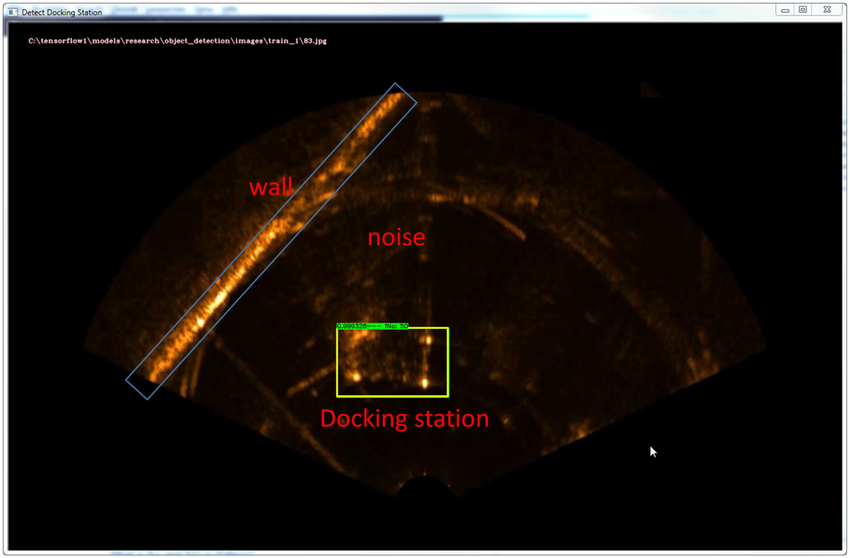
In the underwater realm, it is increasingly important to detect and classify objects such as underwater minerals, e.g., pipelines and cables, mines, corals and docking stations. In this environment, imaging is commonly done by acoustic means due to the benefit of being independent of turbidity. However, their data have some characteristics that make it difficult to process and extract information. These characteristics are non-homogeneous resolution, non-uniform intensity, speckle noise caused by mutual interference of the sampled acoustic returns, acoustic shadowing, and reverberation, and the sonar image construction concept, since the acoustic images are 2D horizontal projections of the observed environment. This fact generates an ambiguity problem because equidistant objects at different heights are mapped to the same position in the acoustic image. The major challenge comes, though, from the difficulty in defining visual features due to limited resolution and very high noise levels. Furthermore, due to the nature of the underwater object detection applications, object detection algorithms need to not only accurately classify and localize important objects, but they also need rapid prediction time to meet the real-time demands using the Autonomous Underwater Vehicle’s (AUV’s) available hardware. Other problems are induced directly by: (1) Dual priorities of object detection, which result from the added goal of object detection that not only do we want to classify image objects but also to determine the objects’ positions. This issue can be addressed by using a multi-task loss function to penalize both misclassifications and localization errors; (2) Underwater target objects in sonar may appear in a wide range of sizes and aspect ratios. There are several methods which practitioners can use to ensure detection algorithms are able to capture objects at multiple scales and views; and (3) Class imbalance also proves to be an issue for underwater object detection. Consider a typical acoustic image such as in Figure 1. More likely than not, the acoustic image contains a few main objects and the remainder of the image is filled with the background or reflections. Recalling that in R-CNN the selective search algorithm produces about 2000 candidate Regions of Interests (RoIs) per image—one can imagine how many of these regions do not contain objects.

Unfortunately, deep learning-based approaches are not well established for acoustic images, mainly due to the scant data in the training phase. Obtaining underwater images is often costly, unlike the abundant publically available air images, and securing enough underwater images for training is not straightforward. Researchers have made many efforts to alleviate the shortage of training data. For example, McKay et al. exploited existing pre-trained weights from in-air images and then applied fine-tuning using sonar images [7]. Further, some authors applied data augmentation from classification, which can have a negative influence on the training results if the augments are not carefully selected. Therefore, in this paper, we use a learned augmentation policy based on reinforcement learning.

There have been multiple research works on underwater object detection in the past. In Alshalali et al., transfer learning was used to fine-tune the pre-trained YOLO model to detect underwater divers [8]. This approach can successfully detect underwater divers with an average frame rate of 45 fps. In Kim and Yu, a method of detecting seabed objects based on machine learning that uses Haar-like features and cascade AdaBoost to analyze side-scan sonar images was proposed [9]. In Lee et al, data augmentation techniques were used to increase the collected training data that were used to train the model. They developed an image synthesizing method to the images captured by an underwater simulator. The synthetic images are based on the sonar imaging models and noisy characteristics to represent the real data obtained from the sea [10]. In [11], Convolutional Neural Networks were applied for object detection in forward-looking sonar images. The authors showed that a CNN outperforms template matching methods by achieving an accuracy of 99.2% compared to between 92.4% and 97.6%. In [12], the authors proposed a method for identifying objects in underwater images based on CNN and Extreme Learning Machine ELM. Hereby, feature extraction is based on CNN and the object classification is based on extreme learning machine. The authors postulated that an ELM was used in the classification stage, because of its generalization ability compared to CNNs. Experiments on a dataset of civil ships obtained a recognition rate of 93.04%.

Furthermore, the considerable successes achieved in object detection in recent years using Machine Learning crucially relies on human–machine learning experts to perform manual tasks (data preparation, feature engineering, model selection, selection of evaluation metrics, and hyperparameter optimization). As the complexity of these tasks for underwater object detection is often beyond non-ML-experts, in this paper we apply principles of Automated Machine Learning to various stages of the machine learning process for the object detector and focus on the following objectives to find solutions of the aforementioned challenges in underwater object detection and at the same time this underlines our min contributions, i.e., (1) Automated underwater data collection and annotation for large datasets, (2) Training for robust detection and precision improvement using learned augmentation policy based on reinforcement learning, (3) Automatic hyperparameter selection based on Bayesian optimization, (4) The design and proof of concept of the object detection methods based on a case study for underwater detection of a docking station in sonar images, (5) The development of a generic underwater object detection system which is independent of the sonar device and carrier platform, and (6) Implementation of the detector on a target hardware (NVIDIA Jetson TX2 Board).

This work has practical implications and implications for future research, because it shows methods for solving basic needs for efficient use of deep learning for underwater object detection, acquisition of large datasets, automatic hyperparameter selection, which is important for non machine learning experts and using appropriate metrics that consider detection and localization accuracy.

The paper is organized into two main sections, the general methodology of the generic concept of underwater object detection and a case study, where the generic detector is applied to detect an underwater docking station. In the methodology part, all the methods developed for our main six contributions previously listed will be described and explained in detail in corresponding subsections. It will start with the methods for a generic underwater object detection system which is independent of the sonar device and carrier platform followed by the other methods for automated underwater data collection and annotation for large datasets, training for robust detection and precision improvement using learned augmentation policy based on reinforcement learning, automatic hyperparameter selection based on Bayesian optimization, and the implementation of the detector on a target hardware (Jetson TX2 Board).

The second part will give the design and proof of concept of the object detection methods based on a case study for underwater detection of a docking station in sonar images. In Section 2 and Section 3, the problem of the case study will be described and the experimental setup as well as the results and discussions will be given, respectively.

2. Methodology

Object detection requires imagery as well as labeled locations of objects that the model can learn from. Therefore, the first step in the workflow illustrated in Figure 2 is obtaining device-independent images from raw sonar data (Section 2.1), followed by data collection and automatic annotation (Section 2.2). The third step is training for object detector robustness (Section 2.3) and the last step is deployment of the trained object detector. All the steps will be described in detail in the following sections, starting with the device-independent image creation block.

2.1. Obtaining Device-Independent Images from Raw Sonar Data

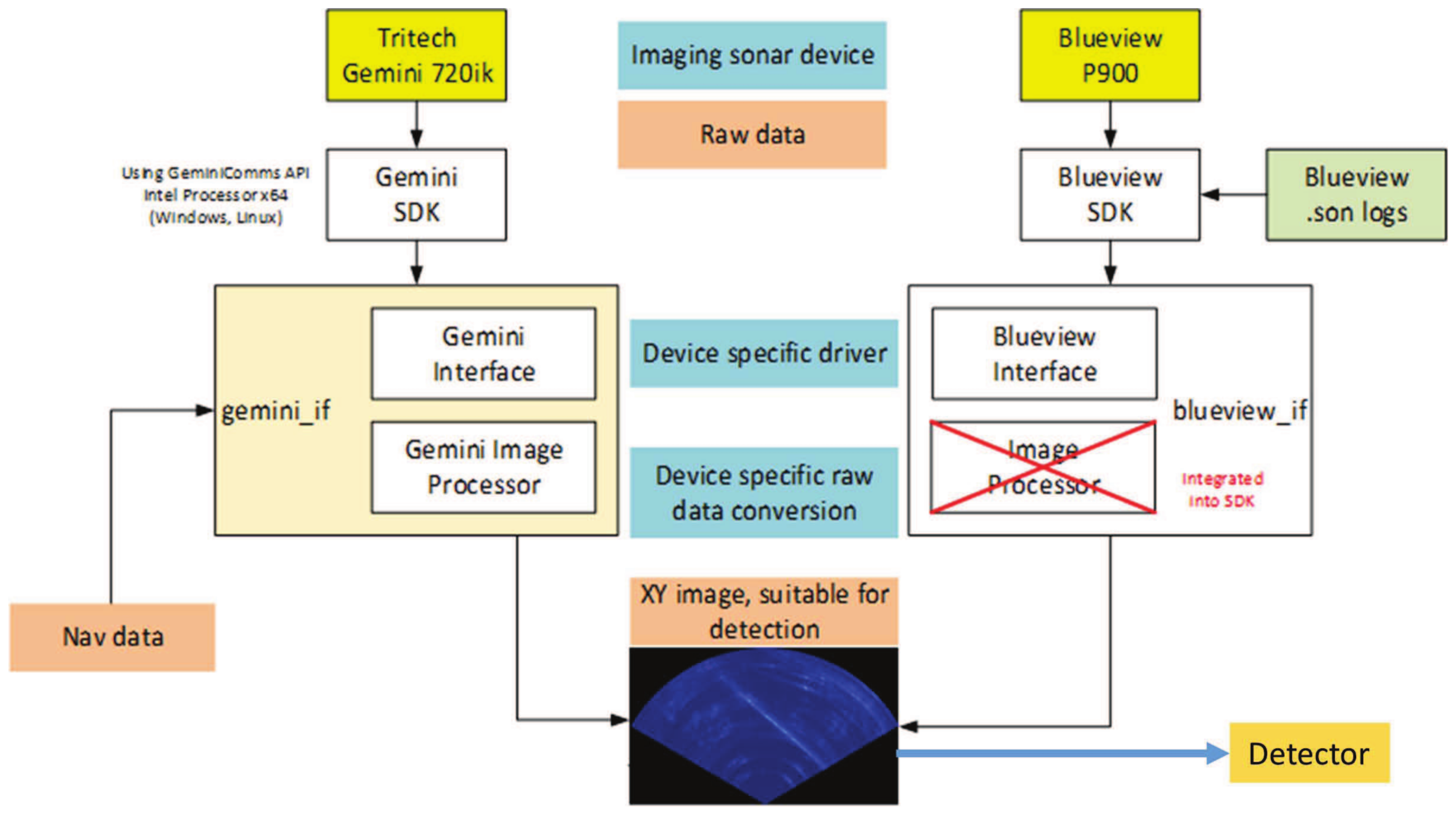
Several imaging sonars exists on the market. Therefore, it is important to develop a detector which is independent of the sonar imaging device to enhance flexibility, as shown in Figure 3. The image shows the workflow to obtain a device-independent XY-Image. The sonar imaging devices, e.g., Gemini 720ik, Blueview 900-130 are controlled by their SDK to generate raw sonar data, which is processed by the image processor to convert RT raw data into XY-Images, which are then fed in, online mode, to the detector.

2.2. Data Acquisition, Augmentation and Annotation of Large Datasets

Collecting underwater images is very difficult and costly. Therefore, this section is dedicated to the problem of limited data and the tedious job of annotating a large amount of data manually. We apply AutoML principles for these tasks and will discuss the following. To tackle the issue of scanty data, we will follow a concept illustrated in Figure 4—Blocks C and E. It takes a sonar image as input. The image can be collected from test basins, sea trials or as planned for the future from a virtual simulator. The image goes randomly over style transfer and the training process is further enhanced with image augmentation. While common practice is to simply use similar augmentation techniques as those done for image classification (flipping, rotation, scaling, etc.) we use specialized augmentations, as part of a ‘learned’ augmentation policy for object detection based on Google Brain’s optimal policy for training [13,14]. We used 3 recommended augmentations, which include (1) rotation—while rotating also means the bounding boxes get larger relative to the object, rotation appears to be the top augmentation, (2) equalize—this operation simply flattens the pixel histogram for the image, and (3) Bounding Box Movement along the Y-axis.

Further, when building datasets for machine learning object detection and recognition models, generating annotations for all of the images in the dataset can be very time consuming and is mainly performed by humans. Therefore, in this section a semi-automatic image collection and annotation method which helps increasing the dataset and annotating images by suggesting annotation for newly captured images will be described. This can significantly speed up the annotation process by the automatic generation of annotation proposals to support the annotator. The structure is shown in Figure 4. It is based on transfer learning, pre-training of a simple detector based R-CNN, and using the simple detector to online to detect while annotating new images for the final training.

Thanks to transfer learning and based on a pre-trained model of similar domain, a simple detector can be trained on a small dataset to obtain satisfactory results. Generally, the idea of transfer learning is to use knowledge obtained from tasks for which a large dataset is available in settings with scanty data like in the underwater environment. Creating labeled data is very cumbersome and expensive. Therefore, leveraging existing datasets is an excellent option. Basically, instead of randomly initializing the starting the learning process, the system learning starts from patterns that have been obtained from a different task that has already been learnt.

Nevertheless, a small dataset needs to be collected. For the underwater object detection, target objects are put in a test basin at known X-Y positions and bounding box sizes. Using a pan and tilt portal crane, which knows its own position in the test basin, a program can be started on the portal crane to move it to different positions while tilting and panning the sonar device. The setup is shown in Figure 5. The sonar head is mounted at the tip point of the portal crane which can pan and tilt move in in all $x,y,z$ directions of the test basin.

First of all the bearing $\theta$ and range R of the corners of the bounding box of the target object are calculated in the test basin coordinate system O relative to the sonar device. Secondly, using the calculated bearing $\theta$, range R and the tilt angle of the sonar head heading ${\varphi }_S$, the distances $d{x}_S\left[m\right]$ and $d{y}_S\left[m\right]$ in the Sonar head coordinate system can be calculated using the following equations.

$$\begin{array}{cc}\hfill d{x}_s& =Rsin(\theta -{\varphi }_s)\hfill \end{array}$$

(1)

$$\begin{array}{cc}\hfill d{y}_s& =Rcos(\theta -{\varphi }_s)\hfill \end{array}$$

(2)

In the third step, $d{x}_S\left[m\right]$ and $d{y}_S\left[m\right]$ are converted to pixel using sonar information (maximum Range set, height H and width W of image obtained) using the following equations.

$$\begin{array}{cc}\hfill d{x}_S\left[pixel\right]& =H\left[pixel\right]\ast d{x}_S\left[m\right]/R_{max}\left[m\right]\hfill \end{array}$$

(3)

$$\begin{array}{cc}\hfill d{y}_S\left[pixel\right]& =H\left[pixel\right]\ast d{y}_S\left[m\right]/R_{max}\left[m\right]\hfill \end{array}$$

(4)

In the final step, the pixel position is obtained in the image coordinate system as follows. In the image with the origin at the top left corner of the image, the position of the sonar head is assumed to be at position $(row=0.5\ast W,col=H)$. Adding $d{x}_S\left[pixel\right]$ and $d{y}_S\left[pixel\right]$ to the position of the sonar head, we get the position of P in the image as $(row=0.5\ast W+d{x}_S\left[pixel\right],col=H-d{y}_S\left[pixel\right])$. The calculations are repeated for every corner of the bounding box of the target object and using the pixel coordinates obtained previously, the image can be annotated to get the XML file. Now, with the simple detector trained on the data from the structured environment (Test basin and portal crane), it can be used to collect a large dataset in an unstructured environment, e.g., sea using a sonar device mounted on an AUV. In this case, images are captured, objects in the images detected and classified and their bounding boxes used for annotation using a Pascal VOC writer. These annotations must be accurate. For this reason, human oversight is required for all of the images in the dataset. It is obvious that the task of only checking and correcting a set of mostly correct annotations is less time consuming than labeling a complete set of images. Consequently, saving a few seconds per image could save several hours of work on a large dataset. For the automatic annotation, a threshold score should be set to suit the dataset and the operator’s needs and should balance the unnecessary annotations against the miss rate. If removing falsely annotated objects is easier for the operator than generating new labels for the missed ones, a lower threshold value should be set to reflect this.

2.3. Designing the Object Detector Based on R-CNN

Generally, before training a deep neural network, the neural network architecture, as well as options of the training algorithm, e.g., training and hyperparameters, should be specified.

We build upon the Fast-R-CNN neural network architecture for object detection, which has been shown to be a state-of-the-art deep learning scheme for generic object detection [4]. Fast-R-CNN is composed of a CNN for feature extraction and RoI network with an RoI-pooling layer and a few fully connected layers for outputting object classes and bounding boxes. Basically, the convolutional network of the Fast-R-CNN takes the whole input image and generates convolutional feature maps as the output. Since the operations are mainly convolutions and max-pooling, the spatial dimensions of the output feature map will change according to the input image size. Given the feature map, the RoI-pooling layer is used to project the object proposals [15] onto the feature space. The RoI-pooling layer crops and resizes to generate a fixed-size feature vector for each object proposal. These feature vectors are then passed through fully connected layers. The fully connected layers output: (i) the probabilities for each object class including the background; and (ii) coordinates of the bounding boxes. For training, the SoftMax loss and regression loss are applied to these two outputs respectively, and the gradients are backpropagated through all the layers to perform end-to-end learning.

Underwater target objects in sonar may appear in a wide range of sizes and aspect ratios. The updated region proposal network of the Faster R-CNN uses, instead of selective search, a small sliding window across the image to generate candidate regions of interest. Multiple RoIs may be identified at each position and are marked with reference to anchor boxes. The anchor boxes have shapes and sizes that are carefully chosen so as to span a range of aspect ratios as well as different scales, which allows objects of various types to be identified hopefully without too much need of bounding box adjustment during the execution of the localization task. Further, a recent approach called focal loss is implemented and helps diminish the impact of class imbalance. It puts more emphasis on misclassified examples, which can make the training more effective and efficient.

The architecture of the Faster R-CNN is clear and is state of the art. The next step is to find the best hyperparameters configuration which gives the best score on the validation/test set. We are faced with the challenge that searching for hyperparameters is an iterative process constrained by computation power, cost and time. Bayesian optimization is an algorithm well suited to optimizing hyperparameters of object detection models because it can be used to optimize functions that are non-differentiable, discontinuous, and time-consuming to evaluate. We choose to optimize the section depth, batch size, initial learning rate, momentum, and L2 Regularization. Momentum adds inertia to the parameter updates by having the current update contain a contribution proportional to the update in the previous iteration. This results in smooth parameter updates and a reduction of the noise inherent to stochastic gradient descent. A good value of L2 regularization helps to prevent overfitting. Data augmentation and batch normalization also help regularize the network.

We created the objective function for the Bayesian optimizer, using the training and validation data as inputs. The objective function trains the Fast R-CNN and returns the classification error on the validation set. Because “bayesopt” [16] uses the error rate on the validation set to choose the best model, it is possible that the final network overfits on the validation set. The resulting model is tested on the unseen test set to estimate the generalization capability.

2.4. Training for Robustness

Training for object detector robustness can be achieved in four ways: (1) Fuzzify objects—intentionally insert noise into the training dataset, for example, target objects are equipped with sonar reflectors of different form and quality and the luminosity of some of the images is varied; (2) Data collection data across target classes as well as the significant variables that contribute to variations. Different hardware (e.g., sonar imaging devices, carrier platforms), for example, are always significant contributors to variation. Therefore, we applied coverage planning to make sure we collected enough and representative data to capture and overcome the variations to be able to train our object detector for robustness. The greater the number of images, the better the accuracy of detection; all kinds of images of the object were taken from different distances, sides and angles using different sonar devices with different qualities for capturing the images; (3) Tuning Hyperparameters using optimization methods and data augmentation using learned policies; and (4) Using a relatively large validation set for training.

2.5. Performance Evaluation Metric

A desirable performance metric should help in setting an optimal confidence score threshold per class and is expected to include all of the factors related with performance, i.e., the localization accuracy of the true positives (TP), the false positive (FP) rate and the false negative (FN) rate. That is why the Average Precision (AP) metric is popular as a performance measure [3,4,5,15]. However, it misses some important performance measures of object detection such as (1) It does not explicitly include the tightness levels of the bounding boxes, which represent the localization accuracy of the true positives which is required in many underwater application such as in underwater mine detection or in our case study where the detected docking station position is used in the docking process that requires position accuracy for rendezvous; (2) It is not sensitive to the confidence score; (3) It does not suggest a confidence score threshold for the best setting of the object detector; and (4) It does not catch the characteristics of different Recall–Precision curves.

To illustrate this, the results of three object detectors on the same image with four sonar reflectors to be detected are shown in Figure 6. In (a) the detector is a low recall–high-precision with only half detections but at maximum precision. In (b) all reflectors are identified with average precision and lastly, in (c), a detector with high precision at low recall and low precision at high recall is presented. Therefore, we introduce a new measure we call the “Bounding box Tightness Level Recall–Precision Error (BTRP)” which includes the terms related to the bounding box tightness level ($IoU$ overlap), recall, precision and each parametrization of $BTRP$ corresponds to a point on the RP curve. We propose the minimum achievable $BTRPerror$, as the alternative metric to AP.

Assuming the object detector has returned the set of bounding boxes Y, we can calculate $BTRP(X,Y_s)$, the BTRP error of $Y_s$ against the set of ground truth boxes X at a given score threshold s$(0\le s\le 1)$ and IoU threshold $\tau$$(0\le \tau <1)$. As done in the calculations for AP, a new set, $Y_s$, containing only the detections that pass the threshold s is created and then, assign the detections in $Y_s$ to ground-truth boxes in X and calculate $TP$, $FP$ and $FN$. Using these quantities, the BTRP error, $BTRP(X,Y_s)$, can be expressed as a weighted function as follows:

$$\begin{array}{cc}\hfill BTRP(X,Y_s)& =\frac{1}{T}\left(\right(TP/(1-\tau )BTR{P}_{IoU}(X,Y_s)\hfill \end{array}$$

(5)

$$\begin{array}{cc}\hfill & +|Y_s|BTR{P}_{FP}(X,Y_s)\hfill \end{array}$$

(6)

$$\begin{array}{cc}\hfill & +\left|X\right|BTR{P}_{FN}(X,Y_s)\left)\right)\hfill \end{array}$$

(7)

where

$$\begin{array}{cc}T\hfill & =(TP+FP+FN)\hfill \end{array}$$

(8)

$$\begin{array}{cc}BTR{P}_{IoU}(X,Y_s)\hfill & =\frac{1}{TP}\sum _{(i=1)}^{TP}(1-IoU(x_i,y\left(x_i\right)))\hfill \end{array}$$

(9)

$$\begin{array}{cc}BTR{P}_{FP}(X,Y_s)\hfill & =\frac{FP}{|Y_s|}\hfill \end{array}$$

(10)

$$\begin{array}{cc}BTR{P}_{FN}(X,Y_s)\hfill & =\frac{FN}{\left|X\right|}\hfill \end{array}$$

(11)

$BTRP$ penalizes each $TP$ by its erroneous localization normalized by $1-\tau$ to the $[0,1]$ interval, each $FP$ and $FN$ by 1 that is the penalty upper bound. This sum of error is averaged by the total number of its contributors, i.e., T. So, with this normalization, BTRP yields a value representing the average error per bounding box in the $[0,1]$ interval. At the extreme cases, a $BTRP$ of 0 means each ground truth item is detected with perfect localization, and if $BTRP$ is 1, then no valid detection matches the ground truth (i.e., $|Y_s|=FP$ ). $BTRP$ is undefined only if there is nothing to evaluate when the ground truth and detection sets are both empty (i.e., $T=0$). Figure 6 shows exemplarily the problems of the AP metric. The figure shows three different object detection results with very different RP curves but the same AP.

3. Case Study

Long underwater operations with autonomous battery charging and data transmission require an AUV with docking capability, which in turn presume the detection and localization of the docking station. Based on the methods described previously in Section 2, we built and implemented an object detector for the detection of an underwater docking station as preparation for control and guidance for AUV docking as follows.

3.1. Implementation

The object detector is based on Google Tensorflow’s object detection API. The target hardware required a C++ API. Therefore, we divided the object detection pipeline into two parts (training and deployment) as shown in Figure 7. Tensorflow’s Python API is a powerful tool that enables everyone to create their own powerful Image Classifiers, visualize the training process (Tensorboard), hence training of the detector was implemented in Python. After training, the frozen graph was optimized using the Graph Optimization Tool (GOT). As described previously in Section 2.2, due to the scanty data for training the simple detector, we applied transfer learning to fine-tune the pre-trained faster_rcnn_inception_v2 Model from the Google Model Zoo. Further, the simple detector was applied online to collect and annotate a larger dataset, which was then used to train the final detector.

The main results, which are in alignment with our objectives for the different challenges in object detection will be presented in the following sections.

3.2. Results and Discussions

3.2.1. Automated Data Collection and Annotation for Large Datasets

The first challenge was how to collect a large number of images of the docking station to contain all kinds of images of the object from all sides and angles for better training. Therefore, a video of the object was taken from all sides. We used two types of sonar devices with different qualities to capture images, namely Blueview P900-130 and a Gemini 720ik. Further, the devices were mounted on different platforms while collecting data, i.e., crane portal, handheld on a pole and mounted on the underwater vehicle ExAUV. Following the procedure in Figure 4, we collected and labeled a small dataset (in this case 1000 images, 500 for training, 300 for validation and 200 for tests), trained a simple object detector using transfer learning to fine-tuned the pre-trained faster_rcnn_inception_v2 model and used Bayesian optimization to find the optimal hyperparameters. The Bayesian search found the following optimal parameters: section depth = 3, batch size = 256, initial learning Rate = 0.1722, momentum = 0.8019 and L2 regularization = 4.2149 × 10${}^{-6}$. We did some experiments with data augmentation for the simple detector. In our system all available 500 training images are automatically augmented using (Rotation, Equalization and Y-Shift) during training. For the simple detector which we trained with manually collected and annotated data, the augmentation showed improved detection rate for unseen images. Without data augmentation, 137 images out of the 200 test images were identified correctly and with data augmenation, 187 out of 200 test images were correctly identified, which gave a significant improvement of 26%.

The trained simple object detector was then used for automatic data collection and annotation of a large dataset. Below are some predictions from the primitive model, which illustrate the benefits of the methodology. Despite having previously trained the model on a very small dataset with only a few training steps, the model makes useful predictions and annotations that save time for manually annotation of the dataset. Figure 8, Figure 9 and Figure 10 show why manual checking of the automatically annotated dataset is necessary and indispensable. For the final detector, the data augmentation did not require much effect to be registered, because with automatic data collection and labeling we already had enough prototypes.

3.2.2. Bayesian Optimization

As we expected, the bigger the batch size the bigger the optimal learning rate found by Bayesian optimization. Using an optimal batch size, which defines the number of training samples that will be propagated through CNN, helps in the reduction of memory use and allows the network to train faster. Since the network is trained with fewer samples, the overall training procedure requires less memory time. On the other hand, the smaller the batch the less accurate the estimate of the gradient will be, as shown in Figure 11a. It can be seen that the direction of the mini-batch gradient fluctuates much more compared to the direction of the full batch gradient. Figure 11b discloses a very interesting characteristic about the relationship, that the noise also increases as the batch size gets smaller. Using a large batch size makes the detector more accurate (mAP for 64 = 0.89 vs. 0.998 for 256) due to the balanced positive and negative examples and its training is nearly an order-of-magnitude faster due to the large learning rate. Bayes optimization compromises between the batch size (it usually requires a large learning rate to maintain accuracy), learning rate (but a learning rate that is too large (required by large batch sizes) in object detection leads to the failure of convergence), and convergence. On the other hand, if a learning rate that is too small is used to ensure the convergence, inferior results are obtained.

3.2.3. Detection

Even though we collected a lot of data with the automatic collection and annotation system, we selected a representative dataset of 2800 images, which we divided into the training and validation sets at the ratio of 4:1. In the 2800 images, 648 very noisy images were also included. All the rest of the data that was automatically collected was then used for tests. After finding the structure of the Faster R-CNN and the optimal hyperparameters, the network was trained with checkpointing for about 6 h on a Dell Latitude E6540 Intel(R) Core(TM) i7-4810MQ CPU @2.80 GHz, 16 GB RAM, Windows 7. The object detector with model size 51 MB took an average of about 1.3 s to process an image with pixel size 960 × 570 and memory capacity 208 kb.

We performed several experiments to test the robustness of the object detector. In the first experiment set, we tested the sensitivity of the object detector to hardware variations (sonar devices, carrier platforms, and reflectors). Four runs were performed, (1) a Blueview P900-130 sonar device was mounted on the tip of a crane portal and in (2) the procedure was repeated using a Gemini 720ik. In (3) Experiment 1 was repeated, but now the carrier platform of the sonar device was an AUV. In (4) Experiment 2 was repeated using an AUV as the carrier platform.

In the second experiment set to test the sensitivity of the object detector to variations to image quality, the Gemini 720ik forward-looking sonar device was mounted on an AUV to perform two experiments where we randomly varied the gain of the sonar device to simulate variations image qualities. Furthermore, we hung several sonar reflectors in the water for more disturbance. In all the experiments we used the performance metric described in Section 2.5. This high accuracy rate suggests that the proposed method is effective and robust for detecting underwater objects.

For the docking station class, $oBTRP$ is determined at the RP pair where there exists a sharp precision decrease on the top right part of the curve. Moreover, this pair provide a Pareto optimum for precision and recall. The detector gives for the docking station class a sharp RP curve (see Figure 12) which corresponds to lower $FP$ and $FN$ error values, which mean excellent detection capabilities. Further, it can be seen that the RP curves do not differ a lot in the 4 experiments, which shows the robustness of the object detector.

Figure 13 and Figure 14 show some representative results of the abovementioned experiments. The visual results in the figures confirm the results in

Table 1. Result of the object detection in 6 experiments, Test 1: Experiment 1 (P900-130 sonar+Portal), Experiment 2 (Gemini+Portal), Experiment 3 (P900-130 on Autonomous Underwater Vehicle (AUV)), Experiment 4 (Gemini on AUV) and Test 2: Experiment 1 (High gain) and Experiment 2 (Reflector noise).

Parameters	Test 1				Test 2
	Exp 1	Exp 2	Exp 3	Exp 4	Exp 1	Exp 2
True targets (TP)	102	208	181	128	1250	1250
Detected targets (FP)	102	208	181	128	1250	1250
False detections(FN)	102	681	208	434	102	319
Average Precision (AP)	0.881	0.845	0.869	0.864	0.788	0.752
oBTRP	0.039	0.151	0.072	0.101	0.212	0.238

. The show true positives with tight bounding boxes independent of the hardware (sonar device, carrier platform) used for data collection or live detection Figure 13b and Figure 13d have more noise than Figure 13a and Figure 13c due to the AUV instabilities. In the case of the experiments of test 2, Figure 14 shows some hard examples with which the system had difficulties. You can see some false positives marked in green. However, their confidence levels are quite low compared to the true positive.

4. Target Hardware

As described previously, the object detector will be running on an AUV. Therefore, we had to test its performance on a target hardware NVIDIA Jetson TX2, with the following technical Specifications GPU 256-core NVIDIA Pascal™ GPU architecture with 256 NVIDIA CUDA cores, CPU Dual-Core NVIDIA Denver 2 64-Bit CPU, Quad-Core ARM^® Cortex^®-A57 MPCore, Memory 8 GB 128-bit LPDDR4 Memory, 1866 MHx—59.7 GB/s, Storage (32 GB eMMC 5.1) and Power (7.5 W/15 W). Figure 15 shows the hardware configuration and the object detector at work. Using the target hardware with GPU, the detection time was reduced from 1.3 s per image to 0.52 s, which is almost a 57% improvement.

The Graph Transformation Tool [17] was applied to optimize the inference. The following transforms were applied: (1) add_default_attributes, (2) strip_unused_nodes, (3) remove_nodes, (4) fold_constants, (5) fold_batch_norms, (6) fold_old_batch_norms, (7) merge_duplicate_nodes, (8) quantize_weights, and (9) quantize_nodes.

Unfortunately, options 1–6 did not produce visible benefits in inference on GPU. The graph memory requirements increased instead and the computation time changed negligibly. With the options quantize_weights and quantize_nodes included, the graph memory requirements reduce drastically from 51 mb to 13 mb but the speed remains the same at very low detection rate. Adding ‘quantize_nodes’ gave us a mismatch on the layers of the model, which made it infeasible to use.

5. Conclusions

A method for building a generic underwater object detection in sonar images has been presented. It tackles several problems along the pipeline of object detection such as automatic annotation, automatic collection of large datasets, hyperparameters optimization, etc. Using the principles of AutoML object detection based on ML can be applied easily by non-machine learning experts. By introducing transfer learning to an R-CNN model, a simple detector was trained and then utilized to collect and annotate a large dataset, which reduced a lot of manual work. The performance of the methods was evaluated on a case study, where the task was to detect an underwater docking station. The detector was robust across different sonar imaging systems and noisy images, which denote that the framework can be considered as an effective detector for underwater objects in sonar images. However, a problem with the proposed method is that it currently takes an average of 1.2 s to process each image. The challenge now is to improve the algorithm to enable online processing in real-time. The results of this study are very significant in the field of underwater detection as automatic data collection and policy-based data augmentation is the prerequisite for efficient object detection in a rough environment, where data is very difficult and expensive to collect.