High Precision Sparse Reconstruction Scheme for Multiple Radar Mainlobe Jammings

Abstract

Radar mainlobe jamming has attracted considerable attention in the field of electronic countermeasures. When the direction of arrival (DOA) of jamming is close to that of the target, the conventional antijamming methods are ineffective. Generally, mainlobe antijamming method based on blind source separation (BSS) can deteriorate the target direction estimation. Thus in this paper, a high precision sparse reconstruction scheme for multiple radar mainlobe jammings is proposed that does not suffer from failure or performance degradation inherent in the traditional method. First, the mainlobe jamming signal and desired signal components are extracted by using the joint approximation diagonalization of eigenmatrices (JADE) method. Then, oblique projection with sparse Bayesian learning (OP-SBL) method is employed to reconstruct the target with high precision. The proposed method is capable of suppressing at most three radar mainlobe jammers adaptively and also obtain DOA estimation error less than 0.1°. Simulation and experimental results confirm the effectiveness of the proposed method.

1. Introduction

Radar systems detect the presence of targets in the background-environment and measure the characteristics of the targets. The purpose of electronic counter-countermeasure (ECCM) is to protect radar systems from electronic countermeasures (ECM) which is often provided by enhanced radar system characteristics, operation and signal processing [1]. In ECM systems, jammings will mask low radar cross-section (RCS) target echoes and degrade radar detection performance. In a conventional phased array radar system, a uniform linear array (ULA) receives a target echo from a surveillance area with the beams pointing towards the interested directions. Jamming signals introduced in the mainlobe direction result in target returns being masked and prevent the weapon system from reaching a launch solution [2,3]. To this end, ECCM is countering the enemy’s ECM to ensure success in the intended mission. Therefore, methods need to be found to suppress mainlobe jamming for a practical radar system. Particularly, the ECCM capability of radar has become a significant indicator of the survivability of modern radar systems.

Mainlobe jamming scenario is illustrated in Figure 1. Various efficient approaches are applied to interfere with the radar mainlobe. Jammings can impinge on the mainlobe or sidelobe of the beam at different beam dwell times. For advanced phased array radar systems, traditional jamming suppression mainly focuses on sidelobe jamming suppression. A variety of techniques can be employed to suppress sidelobe jamming, such as sidelobe blanking, sidelobe cancellation, and ultra-low sidelobe techniques. For the mainlobe jamming, the method of using the blocking matrix processing (BMP) is proposed in [4], but this method will reduce the effective degrees of freedom. The jamming suppression method using eigenprojection matrix processing (EMP) [5] can suppress jamming without loss of freedom, but such a method is also invalid when the jamming is close to the target echo in the arrival direction. Moreover, the application of EMP is limited by the number of jammers. The performance is poor in the case of multiple jammings and aggregation of jamming types. In [6], an adaptive algorithm consisting of adaptive digital beamforming (ADBF) and mainlobe jamming canceller is proposed. This method can suppress both the mainlobe and sidelobe jamming. However, these methods utilizing the spatial sparsity of jamming have a common deficiency in the suppression of multiple mainlobe jammings. For the polarization domain antijamming, it needs every element containing orthogonal polarization channel [7]. However, this method increases the cost and complexity of a practical radar system. The multiple-input–multiple-output (MIMO) radar system with frequency diversity array (FDA) [8,9] was used to suppress mainlobe jamming. However, the FDA-MIMO radar system is limited in practical engineering applications. In [10,11], adaptive sequential estimation was explored to resist mainlobe jamming, however, which is invalid when the waveform of the jamming signal is unknown.

Recently, the blind source separation (BSS) has a good performance on suppressing the mainlobe jamming when the mathematical model fails to be established between the signal source and the sensor, or the prior knowledge is unobtainable. The key idea of BSS is to separate the source signal of the interested target for detection improvement according to the statistical independence of the source signals [12]. When the separated channel of the real target signal is obtained, the antijamming process can be realized.

Three different algorithms based on BSS have been applied to signal separation. The independent component analysis (ICA) algorithm [13] is most widely used to minimize the dependence between the individual signal components [14]. The output vector of principal component analysis (PCA) [15] is obtained by singular value decomposition (SVD) which is used to whiten the input signals and reduce the dimensionality. It has been proved that the PCA algorithm can be used to separate the signals under orthogonal constraints. The key idea of entropy maximization (ME) [16] is to measure the entropy of output information and to maximize the output entropy through iterative optimization.

Some BSS-based approaches have been adopted for mainlobe jamming suppression, a joint approximation diagonalization of eigenmatrices (JADE) algorithm was proposed in [17], which contains the preliminary source processing. However, such a method can suppress the jamming effectively and fail to estimate the correct DOA of the target. The method in [18] has been addressed to obtain the DOA estimation of a low RCS target for phased array radar. However, this method destroys the spatial information of the target. BSS methods have been widely used in resisting multiple mainlobe jammings [19,20,21]. However, these approaches only employ BSS to separate the jamming signals and target returns, which cannot derive the correct DOA of the target. A sparse signal recovery with subarray configuration is capable of suppressing different kinds of jammings and estimating the DOA of the target [22]. However, the accuracy of DOA estimation is not enough.

The main contributions of this work are highlighted as follows:

(1) In the mainlobe jamming suppression field, the key challenge lies in the DOA estimation of the target after jamming suppression. Proposed methods in [4,5,6] can suppress one mainlobe jamming at most in a practical radar system. To overcome this issue, we propose a method using a combination of JADE and OP-SBL [23]. It is shown that using this method the DOA of the target in multiple jammings can be estimated with high precision.

(2) According to the literature, research on BSS can effectively be performed on separating jamming and interested signals. Unfortunately, the BSS method destroys the spatial information of the target. On that basis, we present the OP-SBL method which can suppress the jammings and retain the spatial information of the target dwell time.

(3) Multiple mainlobe jamming suppression capabilities become more important in modern phased array radar systems. In this paper, we take advantage of the source sparse characteristics and spatial adaptive processing. The new method can resist at most three mainlobe jammers and obtain a high accuracy of DOA estimation.

In this paper, a high precision sparse reconstruction scheme for multiple radar mainlobe jammings is proposed. The fourth-order cumulant matrix [24] can be adopted to estimate the steering vector as the preprocessing of mainlobe jamming suppression. Oblique projection operator has been applied to construct the sparse matrix in the next step with the estimated steering vectors. The SBL algorithm has been used to solve the challenging problem of DOA estimation with high precision.

This paper is organized as follows. Section 2 introduces the impact of mainlobe jamming on target detection. The steering vector estimation and sparse reconstruction based on the OP-SBL method are proposed in Section 3. Section 4 offers the results of the simulation to prove the feasibility of the method proposed by the paper, and experimental data collected from a practical radar system is applied to analyze the performance of the suppression method. Finally, the conclusion is drawn in Section 5.

2. Problem Statement

Considering that multiple radar mainlobe jamming suppression and DOA estimation of the target with high precision cannot be achieved simultaneously on a current practical radar model, we propose the following model for analysis. We use a multiple radar mainlobe jammings model based on a practical radar system, which is easy to access.

Suppose that there are $P$ narrowband target signals and $Q$ narrowband mainlobe jamming signals with higher power located at the far-field. $P$ and $Q$ are assumed to know at the receiver. A ULA is focused with $M$ received antennas and $d$ is the spacing between elements of the antenna array.

The target signals and jamming signals are statistically independent. The received signal of $m$-th array element can be expressed as

$$\begin{array}{cc}\hfill x_m(t)=& {\displaystyle \sum _{p=1}^P{\alpha }_{T,p}{s}_p(t)\exp \left[-j(m-1)\frac{2\pi d}{\lambda }\sin {\theta }_{T,p}\right]}\hfill \\ \hfill & +{\displaystyle \sum _{q=1}^Q{\alpha }_{J,q}{j}_q(t)\exp }\left[-j(m-1)\frac{2\pi d}{\lambda }\sin {\theta }_{J,q}\right]+n_m(t),m=1,2,\dots ,M\hfill \end{array}$$

(1)

where ${\alpha }_{T,p}$ is the complex amplitude parameter accounting for the $p$-th target RCS, channel propagation effects involved in the radar range equation, $s_p(t),p=1,2,\cdots ,P$ and $j_q(t),q=1,2,\cdots ,Q$ are target signals and jamming signals, ${\theta }_{T,p}$ is the DOA of the $p$-th target signal, ${\alpha }_{J,q}$ and ${\theta }_{J,q}$ are the complex amplitude parameter and the DOA of the $q$-th mainlobe jamming, $n_m(t)$ denotes the zero-mean additive white Gaussian noise with variance ${\sigma }_m^2$ and $\lambda$ is the operating wavelength.

The received signals are collected into a vector which can be expressed by

$$X(t)=A_T{S}_T(t)+A_J{S}_J(t)+N(t)=A_{hybrid}S(t)+N(t)$$

(2)

where $X(t)={\left[x_1(t),x_2(t),\cdots ,x_M(t)\right]}^T$ denotes array received signal vector and ${[·]}^T$ denotes transpose, $A_T=\left[a\left({\theta }_{T,1}\right),\cdots ,a\left({\theta }_{T,P}\right)\right]$ represents the steering vector of the target and

$a\left({\theta }_{T,p}\right)={\left[-1,-j\frac{2\pi d}{\lambda }\sin \left({\theta }_{T,p}\right),\cdots ,-j(m-1)\frac{2\pi d}{\lambda }\sin \left({\theta }_{T,p}\right)\right]}^T$ is the steering vector of the $p$-th target. $S_T(t)={\left[{\alpha }_{T,1}{s}_1\left(t\right),\cdots ,{\alpha }_{T,P}{s}_P\left(t\right)\right]}^T$ stands for the target signal vector, $A_J=\left[a\left({\theta }_{J,1}\right),\cdots ,a\left({\theta }_{J,Q}\right)\right]$ represents the steering vector of the jamming, $S_J(t)={\left[{\alpha }_{J,1}{j}_1\left(t\right),\cdots ,{\alpha }_{J,Q}{j}_Q\left(t\right)\right]}^T$ stands for the jamming signal vector, $A_{hybrid}$ is a $M\times (P+Q)$ dimensional hybrid matrix which can be represented as $A_{hybrid}=[A_T,A_J]$, $S(t)={\left[{\alpha }_{T,1}{s}_1\left(t\right),\cdots ,{\alpha }_{T,P}{s}_P\left(t\right),{\alpha }_{J,1}{j}_1\left(t\right),\cdots ,{\alpha }_{J,Q}{j}_Q\left(t\right)\right]}^T$ is a $P+\mathrm{Q}$ dimensional received signal vector denoted as $S(t)={\left[S_T(t),S_J(t)\right]}^T$ and $N(t)$ denotes the Gaussian white noise vector.

3. Methodology

In this section, a steering vector estimation method is proposed that relies on a diagonalized fourth-order cumulant matrix to separate the target and jamming signals. Then, the OP-SBL method is applied to construct the sparse reconstruction matrix and estimate the DOA of the target.

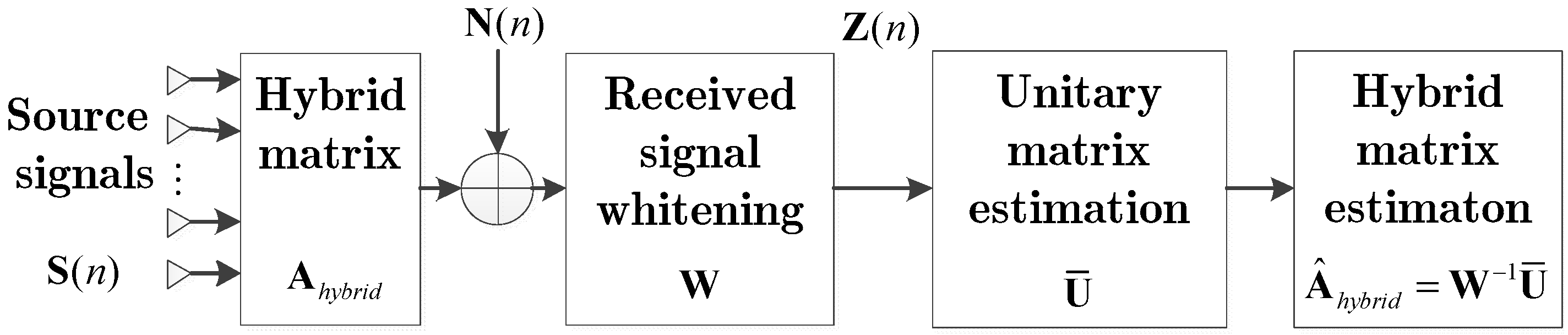
3.1. Steering Vector Estimation Based on Fourth-Order Cumulant Matrix

The JADE algorithm uses the fourth-order cumulant property of multi-dimensional data to separate the independent signals and the eigenvalue decomposition of the fourth-order cumulant matrix is used to estimate the hybrid matrix. The algorithm transforms the objective function maximization problem into diagonalizing a set of fourth-order cumulant matrix eigenvalues. The joint diagonalization approach improves the efficiency of our algorithm.

For the premise of the JADE algorithm to effectively separate the sources, we suppose that the number of the sources is less than the number of receiving channels, i.e., $(P+Q)\le M$, and the hybrid matrix has a full column rank.

The basic flowing diagram of the algorithm is shown in Figure 2.

Step 1: Sample the received signal $X(t)$ in the time domain and it can be written as $X(n)=A_{hybrid}S(n)+N(n)$, where $n$ is the discrete sample point.

Step 2: Whiten the received signal $X(n)$:$Z(n)=WX(n)$ where $W$ is the whitening matrix. The covariance matrix of the received signal can be written as

$$R_X=E\left[X(n)X^H(n)\right]$$

(3)

Perform eigenvalue decomposition on the received signal covariance matrix $R_X$, $R_X=\Gamma \Lambda {\Gamma }^H$ will be obtained, while the covariance matrix of $Z(n)$ should be an identity matrix by the whitening process.

$$I=R_Z=E\left[Z(n)Z^H(n)\right]=E\left[WX(n)X^H(n)W^H\right]=W{R}_X{W}^H=W\Gamma \Lambda {\Gamma }^H{W}^H$$

(4)

Denote a whitening matrix $W={\Lambda }^{-1/2}{\Gamma }^H$, where $\Lambda$ is the eigenvalue matrix and $\Gamma$ is the corresponding eigenvector matrix.

The signal after the whitening process can be written as

$$Z(n)=WX(n)=US(n)+WN(n)$$

(5)

where the unitary matrix is denoted as $U=W{A}_{hybrid}$.

Hence, the covariance matrix $R_Z$ can be written as

$$\begin{array}{cc}\hfill R_Z& =E\left[Z(n)Z^H(n)\right]=E\left[\left(US(n)+WN(n)\right){\left(US(n)+WN(n)\right)}^H\right]\hfill \\ \hfill & =E\left[US(n)S^H(n)U^H+WN(n)N^H(n)W^H\right]\hfill \end{array}$$

(6)

The amplitude of the source signals is represented by the column vector of the hybrid matrix and we suppose there are $K$ source signals. Hence, the source signals have a unit variance $E\left[s_k(n)s_k^H(n)\right]=1$ for $k=1,\cdots ,K$, the covariance matrix $R_Z$ can be rewritten as

$$R_Z=U{U}^H+{\sigma }_N^{2}WI{W}^H$$

(7)

where ${\sigma }_N^2$ is the power of noise, ignore the effect of noise and (7) can be approximated as

$$R_Z\approx U{U}^H$$

(8)

According to (8), the unitary matrix $U$ should be estimated for recovering source signals.

Step 3: Estimate unitary matrix

Let $u_m$ be the $m$-th column of the unitary matrix $U$, hence $u_m$ can be written as

$$u_m={\left[\begin{array}{cccc}{u}_{m1}& u_{m2}& \dots & u_{mK}\end{array}\right]}^T$$

(9)

Assume that $\Omega =u_m{u}_m^T$, the $k$-th raw and $l$-th column element of a matrix $\Omega$ can be written as ${\mathsf{\Omega }}_{kl}=u_{mk}{u}_{ml}$.

$$S(n)={\left[s_1(n),\cdots ,s_q(n),\cdots ,s_K(n)\right]}^T$$

(10)

where $s_q(n)$ is the $q$-th source of $S(n)$.

The eigenmatrix and eigenvector can be obtained by eigendecomposition of fourth-order cumulant matrix ${\left[Q_Z(\Omega )\right]}_{ij}$ which can be written as

$${\left[Q_Z(\Omega )\right]}_{ij}=\overline{U}\Sigma {\overline{U}}^H$$

(11)

where $\Sigma$ is the eigenmatrix of the fourth-order cumulant matrix. Then the unitary matrix $\overline{U}$ can be obtained. The proof of the eigendecomposition of the fourth-order cumulant matrix is provided in Appendix A.

Step 4: Achieve the estimation of the steering vector

$${\widehat{A}}_{hybrid}=W^{-1}\overline{U}$$

(12)

Accordingly, the estimation of the hybrid matrix ${\widehat{A}}_{hybrid}$ can be dealing with the unitary matrix $\overline{U}$. The steering vector of target and jamming can be obtained by the estimated hybrid matrix.

3.2. Sparse Reconstruction with Jamming Suppression Based on OP-SBL Algorithm

After hybrid matrix estimation, we can get $\widehat{S}(n)$ from the source signals which consist of a target signal’s estimation ${\widehat{S}}_T(n)$ and the jammings’ estimation ${\widehat{S}}_J(n)$. Besides, the estimated hybrid matrix ${\widehat{A}}_{hybrid}$ is composed of the estimated steering vectors ${\widehat{A}}_T(\theta )$ of the target and the estimated steering vectors ${\widehat{A}}_J(\theta )$ of the jamming. Then, the oblique projection operator is applied to suppress the jamming.

Let us denote

$$\begin{array}{l}Q\triangleq {\widehat{A}}_T(\theta )\\ H\triangleq {\widehat{A}}_J(\theta )\end{array}$$

(13)

The difference between the steering vectors of target and jammings can be obtained by pulse compression. Denoting $P_Q=Q{Q}^{+}$ is the projection matrix of $Q$, where $Q^{+}={(Q^{H}Q)}^{-1}{Q}^H$. $P_Q^{\perp }=I-P_Q$ is the orthogonal projection matrix of $Q$. The oblique projection matrix $E_{QH}$ is the projection operator from subspace $H$ to $Q$, which is denoted as

$$\begin{array}{cc}{E}_{QH}\hfill & =\left[\begin{array}{cc}Q& 0\end{array}\right]{\left[\begin{array}{cc}{Q}^{H}Q& Q^{H}H\\ H^{H}Q& H^{H}H\end{array}\right]}^{†}\left[\begin{array}{c}{Q}^H\\ H^H\end{array}\right]\hfill \\ \hfill & =Q{(Q^H{P}_H^{\perp }Q)}^{-1}{Q}^H{P}_H^{\perp }\hfill \end{array}$$

(14)

where $P_H^{\perp }=I-H{\left(H^{H}H\right)}^{-1}{H}^H$ is the orthogonal projection operator and ${\{\cdot \}}^{†}$ denotes the generalized inverse of the matrix.

Hence, the oblique projection processing can be expressed as

$$X_{ob}(n)=E_{QH}X(n)$$

(15)

The results after oblique projection processing are reconstructed to estimate the angular parameters by the SBL method.

When the JADE algorithm is applied to obtain the steering vector and the estimated signal of the target, the whitening characteristic is also affecting the recovery of the amplitude of the original signal. Conventional methods fail to obtain the DOA information of the target. The energy of target will also be weakened owing to the separation process. Therefore, it leads to a large error in the direction estimation of the target by using the separated channel data for subsequent processing. The purpose of oblique projection is to suppress the jamming energy and maximize the detection probability of the target.

However, the unsuppressed jammings and noise are still contained in $X_{ob}(n)$. This part of the signal can be regarded as noise uniformly. SBL is used to obtain target parameters that contain the DOA of the target.

The residual noise is considered in the $X_{ob}(n)$ and the noise is denoted as $V(n)$, (15) can be rewritten as

$$X_{ob}(n)={\tilde{A}}_T(\theta ){\tilde{S}}_T(n)+V(n)$$

(16)

where ${\tilde{A}}_T(\theta )$ stands for the steering vector of a recovered signal of the target, ${\tilde{S}}_T(n)$ represents the estimation of real target echo.

Then, the SBL is performed to estimate the angular parameter of the target and an overcomplete basis dictionary is represented as

$$\Phi =\left[a({\tilde{\theta }}_1),\cdots ,a({\tilde{\theta }}_N)\right]$$

(17)

where ${\left\{{\tilde{\theta }}_n\right\}}_{n=1}^N$ represents the samples of the spatial-temporal features, the sampling range is $\left[-\pi /2,\pi /2\right]$ and the sparse expression of the direction estimation can be obtained as

$$r(n)=\Phi \omega (n)+e(n)$$

(18)

where the steering vector corresponding to $\tilde{\theta }$ is composed of the array manifold $\Phi$ and $\omega$ represents the sparse coefficient matrix. Assume that the angle of incidence is fixed during the entire observation period. When ${\theta }_m$ of the $m$-th signal equals to the ${\tilde{\theta }}_k$, the $k$-th row elements of $X$ is nonzero. Once the nonzero position of $X$ is determined, the DOA of the signal can be calculated from the position corresponding to $\tilde{\theta }$. This relation forms the basis of the sparse representation algorithm.

The objective function of the conventional sparse expression is written as

$${\omega }_{opt}(\lambda )=\arg \underset{\omega }{\min }\left({\Vert r-\Phi \omega \Vert }_2^2\right)+\lambda {\Vert \omega \Vert }_1$$

(19)

where ${\Vert ·\Vert }_2$ denotes the $l_2$ norm, ${\Vert ·\Vert }_1$ denotes the $l_1$ norm and $\lambda$ is the positive regularization parameter.

The sparse Bayesian learning central idea is based on the empirical Bayesian principle and specifically converts the objective function of conventional sparse expression into the objective function of sparse Bayesian expression.

$${\omega }_{opt}(\lambda )=\arg \underset{\omega }{\max }p(\omega |r)$$

(20)

where $p(\omega |r)$ represents the posterior probability distribution of $\omega$.

Assume that the observation noise is complex Gaussian white noise, the likelihood function of the observation model can be expressed as

$$p(r|\omega ;{\sigma }^2)={\left(2\pi {\sigma }^2\right)}^{-ML/2}\exp \left(-\frac{1}{2{\sigma }^2}{\displaystyle \sum _{l=1}^L{\Vert r_l-\Phi {\omega }_l\Vert }_2^2}\right)$$

(21)

where $L$ represents the training number of the observation samples, $r_l$ is the $l$-th column sample of the $r$, ${\omega }_l$ is the sparse coefficient and ${\sigma }^2$ is the variance of the noise. Each column of the $\omega$ is assumed to follow a zero-mean complex Gaussian distribution defined as ${\omega }_l~{\rm N}(0,\psi )$, where $0\in C^{M\times 1}$, $\psi =diag(\gamma )$, $\gamma ={\left[{\mathsf{\gamma }}_1,\cdots ,{\mathsf{\gamma }}_N\right]}^T$ represents the variance of sparse coefficient in a different angle. Therefore, the prior distribution about the sparse coefficient can be expressed as

$$p\left(\omega ;\psi \right)={\pi }^{-NL}{\psi }^{-L}\exp \left(-{\displaystyle \sum _{l=1}^L{\omega }_l^H{\psi }^{-1}{\omega }_l}\right)$$

(22)

According to the joint likelihood function and the prior distribution, the obtained posterior probability distribution can be derived as

$$p\left(\omega |r;\psi ,{\sigma }^2\right)=\frac{p\left(r,\omega ;\psi ,{\sigma }^2\right)}{{\displaystyle \int p\left(r,\omega ;\psi ,{\sigma }^2\right)d\omega }}=\frac{p\left(r|\omega ;{\sigma }^2\right)p\left(\omega ;\psi \right)}{{\displaystyle \int p\left(r|\omega ;{\sigma }^2\right)p\left(\omega ;\psi \right)d\omega }}$$

(23)

The problem of direction estimation can be solved when obtaining the nonzero elements in the sparse coefficient. The variance represents the energy of the signal.

The method of expectation maximization (EM) is used to estimate the sparse coefficient and the variance of the noise. The likelihood estimation is corrected by iterative updating.

Suppose that ${\psi }_i$ and ${\sigma }_i^2$ are known, the posterior probability distribution of the sparse coefficient calculated from the posterior probability density distribution can be represented as

$$\begin{array}{cc}\hfill p\left({\omega }_{i+1}|r;{\psi }_i,{\sigma }_i^2\right)& =\frac{p\left(r|{\omega }_{i+1};{\sigma }_i^2\right)p\left({\omega }_{i+1};{\psi }_i\right)}{{\displaystyle \int p\left(r|{\omega }_{i+1};{\sigma }_i^2\right)p\left({\omega }_{i+1};{\psi }_i\right)d{\omega }_{i+1}}}\hfill \\ \hfill & ={\left|\pi {\Sigma }_{i+1}\right|}^{-NL}\exp \left\{-tr[{({\omega }_{i+1}-U_{i+1})}^H·{\Sigma }_{i+1}^{-1}({\omega }_{i+1}-U_{i+1})]\right\}\hfill \end{array}$$

(24)

where ${\Sigma }_{i+1}$ is the covariance matrix in the $i+1$-th step which is denoted as

$${\Sigma }_{i+1}={\psi }_i-{\psi }_i{\Phi }^H{\left({\sigma }_i^{2}I+\Phi {\psi }_i{\Phi }^H\right)}^{-1}\Phi {\psi }_i$$

(25)

$U_{i+1}$ is the average vector denoted as

$$U_{i+1}={\psi }_i{\Phi }^H{\left({\sigma }_i^{2}I+\Phi {\psi }_i{\Phi }^H\right)}^{-1}r$$

(26)

In the EM step, it is required to maximize the expectation in the case of obtaining the posterior distribution. The following optimization objective function equation can be obtained.

$$\left[{\mathsf{\gamma }}_{i+1},{\sigma }_{i+1}^2\right]=\arg \underset{\psi ,{\sigma }^2}{\max }E\left[\ln p\left({\omega }_{i+1}|r;{\psi }_i,{\sigma }_i^2\right)\right]$$

(27)

Employing the values $\mathsf{\gamma }$ and $\sigma$ to update until the iteration stopping criterion ${\Vert {\mathsf{\gamma }}_{i+1}-{\mathsf{\gamma }}_i\Vert }_2/{\Vert {\mathsf{\gamma }}_{i+1}\Vert }_2\le \delta$ is satisfied.

$${\mathsf{\gamma }}_{n,i+1}=\frac{1}{L}{\Vert U_{n,i+1}^{(l)}\Vert }_2^2+{\Sigma }_{n,i+1}$$

(28)

$${\sigma }_{i+1}^2=\frac{1/L{\Vert r-\Phi {\omega }_{i+1}\Vert }_2^2}{M}+\frac{{\sigma }_i^2{\displaystyle {\sum }_{n=1}^N\left(1-{\Sigma }_{n,i}/{\mathsf{\gamma }}_{n,i}\right)}}{M}$$

(29)

$\tilde{\omega }(n)$ corresponding to the DOA of the target can be obtained by the SBL algorithm.

The flowchart of the method is summarized as Figure 3. According to the statistical independence between the source signals, they are separated by the JADE algorithm. The OP-SBL algorithm is used to suppress the jamming and estimate the DOA of the target efficiently.

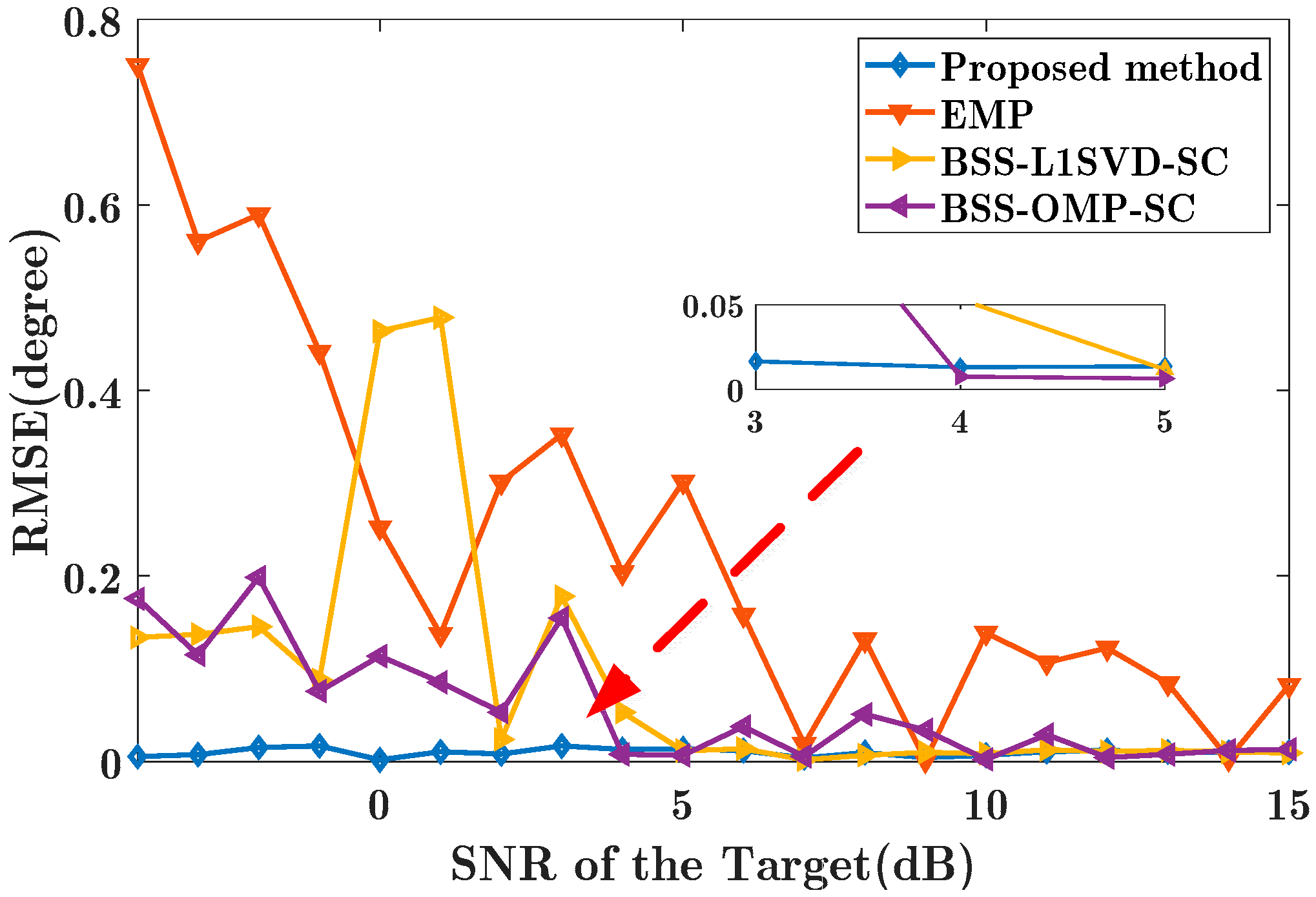
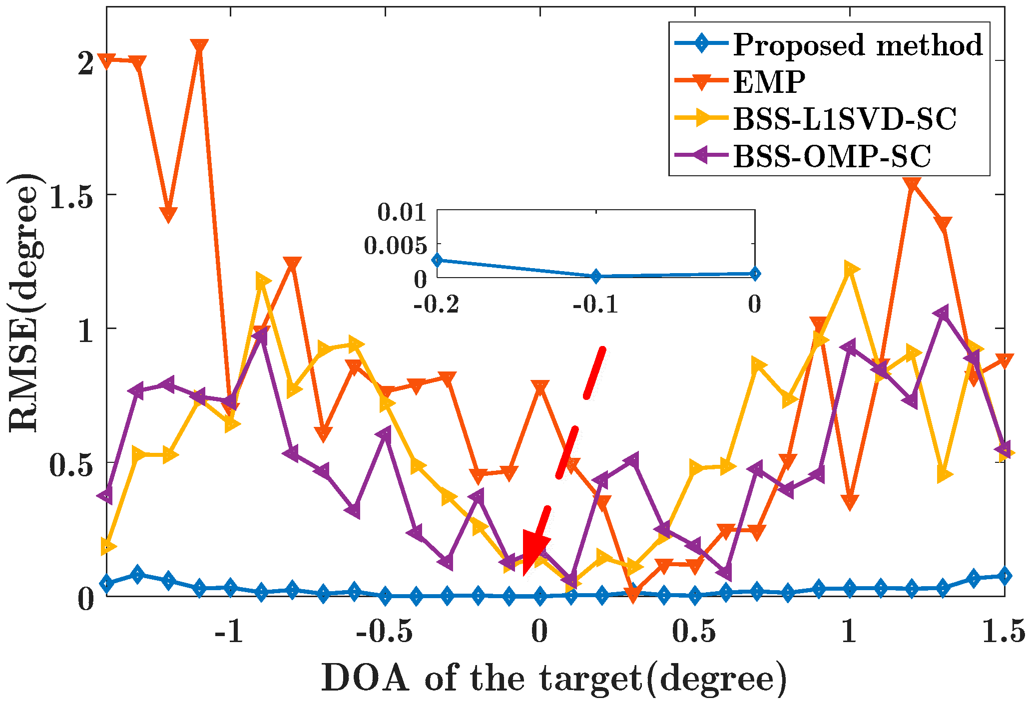
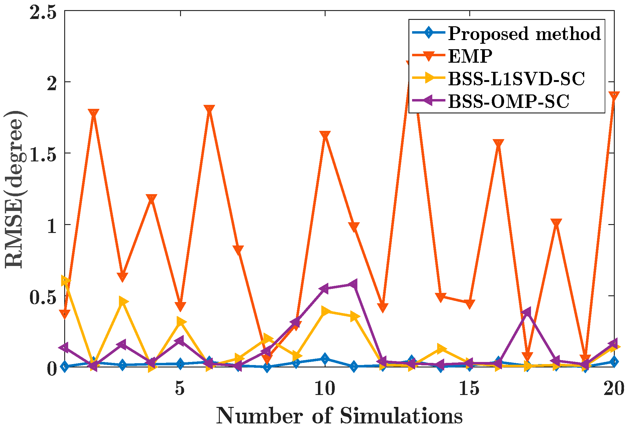
4. Experimental Results

To assess the performance of the proposed method, we conduct computer simulations based on a PC with Intel i5-8250u CPU and RAM 8 GB, employing MATLAB (version R2018a, 64 bit).

In this section, numerical simulation results and experimental data verification results are shown to evaluate the effectiveness of jamming suppression and the accuracy of DOA estimation.

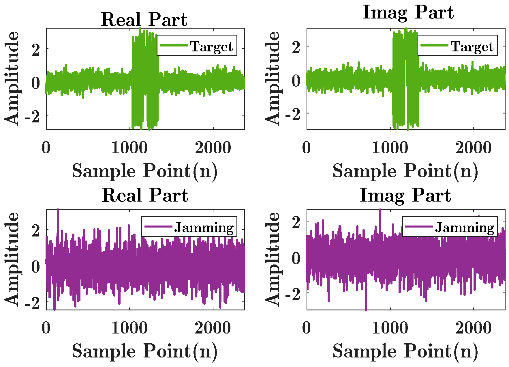
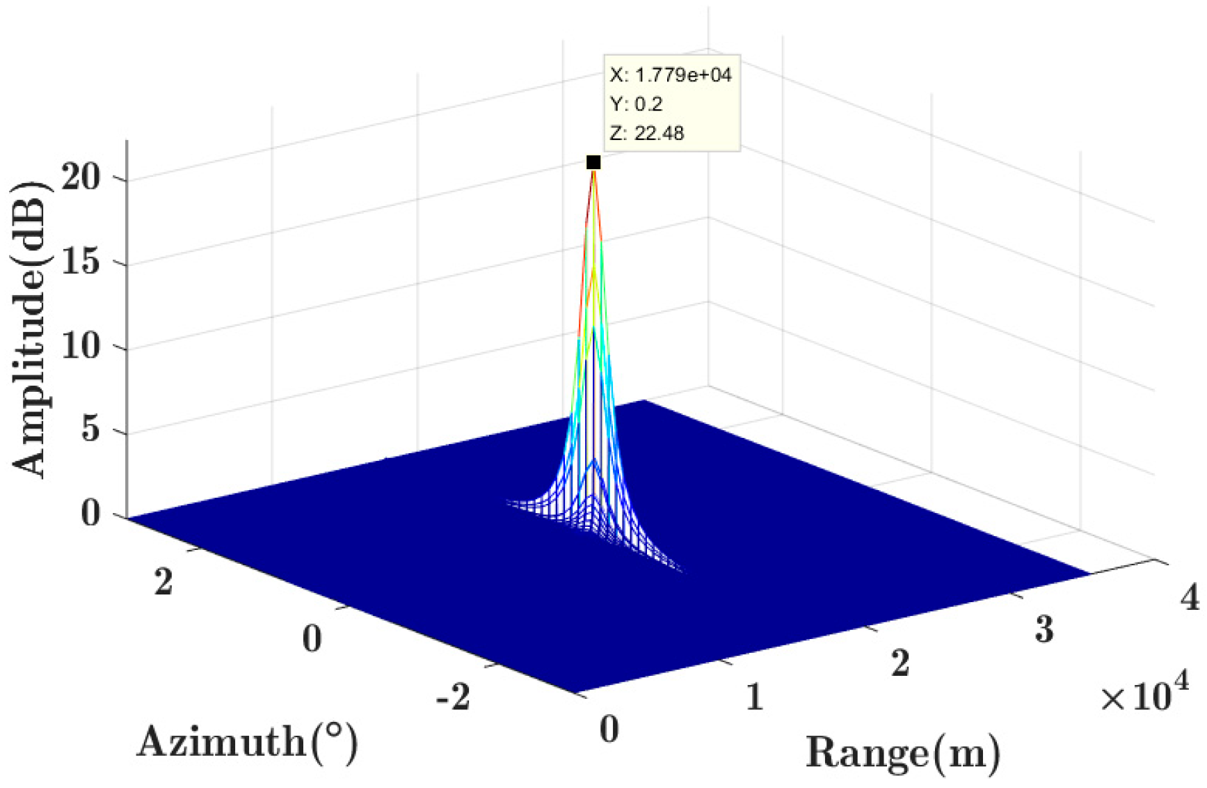
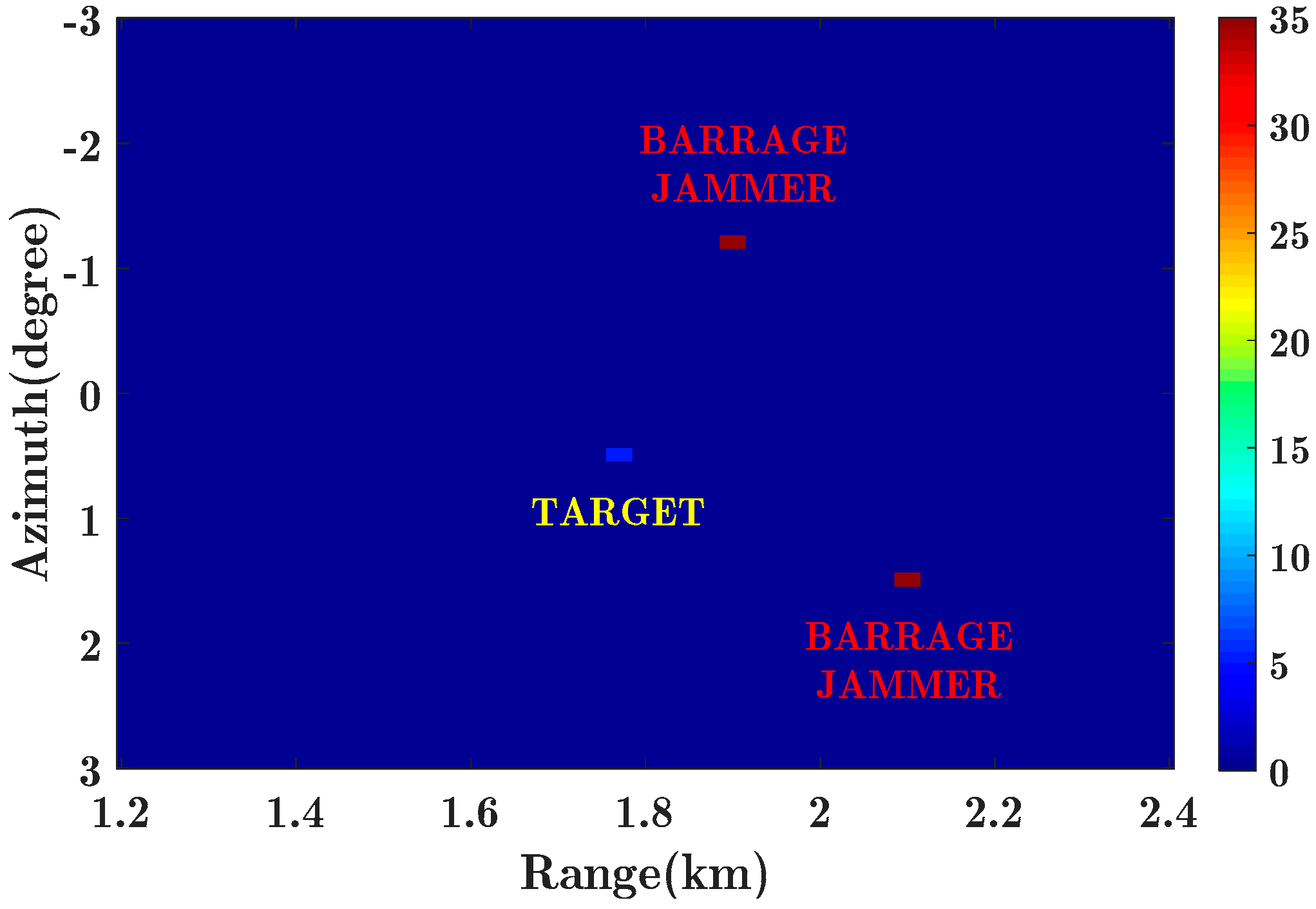
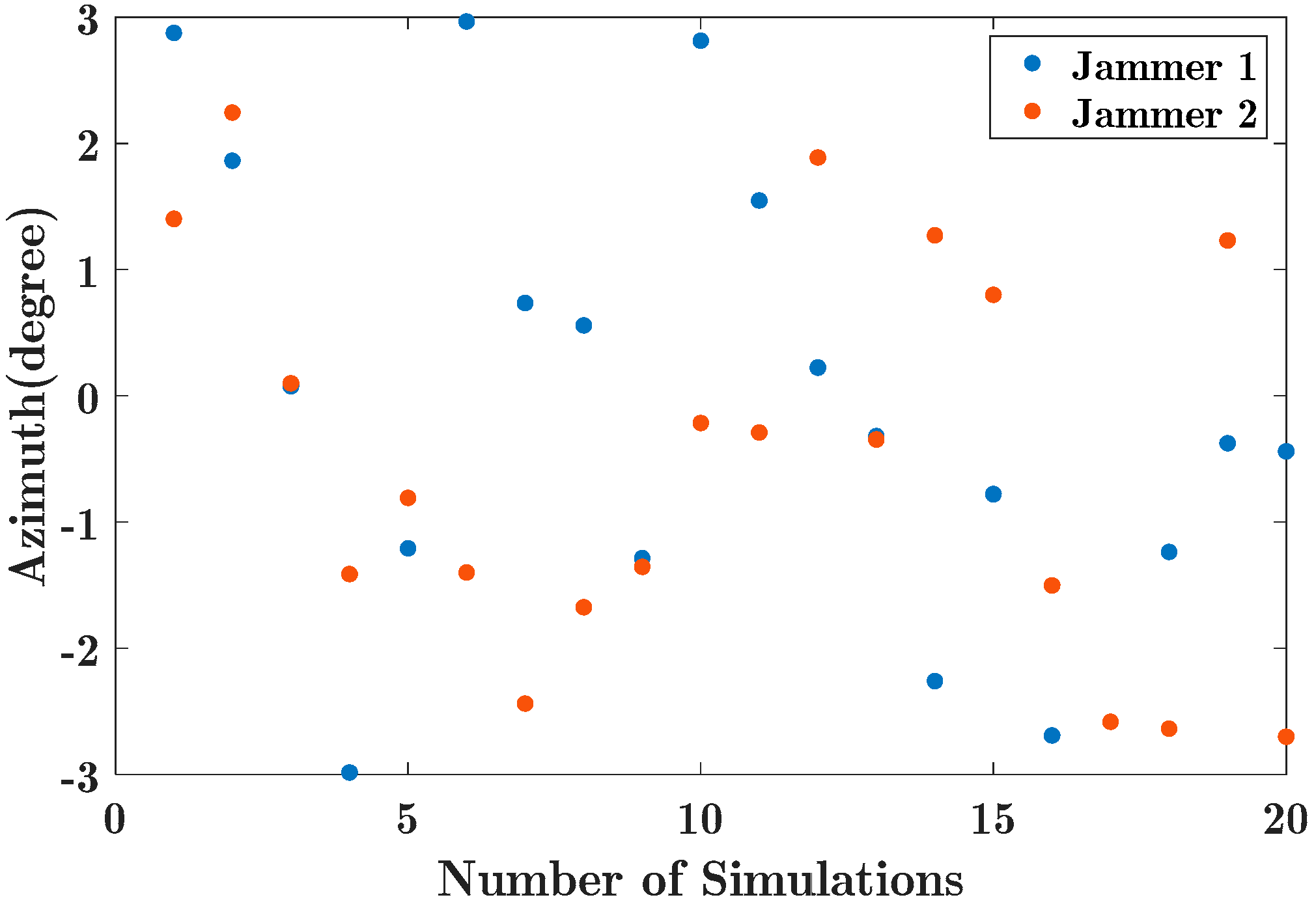
4.1. Simulation Study

Let us suppose a linear array which has 16 elements placed half a wavelength apart. The transmitted signal is the pulsed LFM signal, with bandwidth 5 MHz, pulse width 30 µs, and sampling rate 10 MHz. The target comes from the azimuth angle of $0.2°$ and is located at 17.79 km. The noise in each channel follows the additive white Gaussian noise. The 3 dB azimuth beamwidth is $6.33°$. The number of spatial channels is 16. The initial phase of the target and jamming observe uniform distribution $U(-\pi ,\pi )$.

Assume the barrage jamming signal in the mainlobe is a noise amplitude modulated signal. They can be expressed as

$$j_{BA}(t)=\left[{\alpha }_J+\chi (t-{\tau }_J)\right]\exp \left(j2\pi f_0(t-{\tau }_J)+j{\phi }_J\right)$$

(30)

where $\chi (t)$ is the amplitude modulation of the barrage jamming signals which is a wide-sense stationary random process with Rayleigh distribution. ${\tau }_J$ and ${\phi }_J$ is the time delay and initial phase of the jamming.

Suppose that there is one target and one mainlobe jammer received from the far-field. The SNR of the target is set at 5 dB and the JSR is set at 30 dB. The mainlobe jamming coming from $0.2°$ is assumed.

Besides, the SNR of the target is defined as

$$SNR=10{\log }_{10}\left(\frac{{\alpha }_T^2}{{\sigma }_N^2}\right)$$

(31)

JSR of the barrage jamming can be defined as

$$JSR=10{\log }_{10}\left(\frac{{\alpha }_J^2+{\chi }^2}{{\alpha }_T^2}\right)$$

(32)

The root mean square error (RMSE) is defined as

$$RMS{E}_{\theta }=\sqrt{{\displaystyle \sum _{d=1}^D{\displaystyle \sum _{p=1}^P{\left({\widehat{\theta }}_p(d)-{\theta }_p\right)}^2/P}}D}$$

(33)

where ${\widehat{\theta }}_p(d)$ is the estimation of ${\theta }_p$ in the $d$-th trial and $D$ is the number of the Monte Carlo simulation.

First, the time domain output result of the synthesis linear array beam is presented in Figure 4. It can be seen from Figure 4 that the target is completely submerged in the jamming. The two channel results after separation processing are given in Figure 5. The target and jamming are well separated by the JADE algorithm. However, the amplitude information of the target has also been changed. DOA estimation will be affected by the amplitude error.

From Figure 6, the purple curve plots the result of the original signal after the matched filter. It is shown the target is submerged in the jamming. The green curve plots the result of oblique projection processing. As expected, the output of the target echo appears as peaks so that the target can be easily detected. It is found that the amplitude information of the target can be obtained successfully and suppression of the jamming has been achieved. Therefore, the OP method can successfully achieve high power barrage jamming suppression.

The OP-SBL method is used to estimate the DOA of the target. As we can see from Figure 7, the target locates at an azimuth angle of $0.2°$ which amplitude is over 20 dB. The estimated DOA of the target is basically consistent with the simulation parameters.

To further verify the validity of the proposed method in jamming suppression. Assume that the jamming environment exists two barrage jammers as Figure 8 shows. The SNR of the target is 5 dB at $0.5°$ where it is located. The JSRs are 32 dB and 35 dB of the jammers, respectively. The angles are set at $-1.3°$ and $1.5°$. The angle between the target and the second jammer in azimuth is $1°$ which is 1/6 of the mainlobe beamwidth.

As is shown in Figure 9, the accuracy of DOA estimation is compared under the condition of different SNR input of the target. Compared with the proposed method, EMP, BSS-OMP-SC and the method proposed in [22] about the DOA estimation of the target. It is obvious that the proposed method illustrates the RMSE of our method less than $0.1°$ when SNR input of the target is higher than −5 dB. The RMSE of target estimation by using the BSS-L1SVD-SC method is less than $0.1°$ when the SNR input of the target is greater than 5 dB. EMP is unable to estimate the DOA of the target while there are two mainlobe jammers. Specifically, the RMSE of the proposed method is lower than other methods under high SNR.

Then, we analyze the performance of DOA estimation in every direction when the target is moving. The jamming environment is shown in Figure 10. The target moved from $-1.5°$ to $1.5°$ which is 1/2 of the mainlobe beamwidth and the SNR input of the target is 5 dB. The JSRs of two barrage jammers are 32 dB and 35 dB, respectively. The angles are set at $-1.3°$ and $1.5°$. We use the RMSE to evaluate the accuracy of DOA estimation of the target which is analyzed in Figure 11. All the results are the statistical average of the 100 times of Monte Carlo simulation.

As Figure 11 shows, the proposed method depicted by a blue line is compared with EMP, BSS-L1SVD-SC and BSS-OMP-SC. Obviously, it can be seen the proposed method maintains a good performance in DOA estimation while the other methods have failed when the angle between the target and jamming decreases. The BSS-L1SVd-SC is applicable when the target moves around $0°$ and the angle between target and jammer is over 1/4 mainlobe beamwidth. The proposed method can successfully estimate the DOA of the target in two barrage jammers and the RMSE of the proposed method is lower than other methods. Moreover, the RMSE of the proposed method keeps stable with the angle between target and jamming decreasing.

We fix the target located at $0.5°$, prepare 20 experiments by using randomized locations for jammers within the mainlobe beamwidth and repeat the performance analysis of DOA estimation. The jammers’ locations are shown in Figure 12. All the results are the statistical average of the 100 times of Monte Carlo simulation.

As shown in Figure 13, the method in this paper is still effective and superior to other algorithms. EMP method fails to estimate the DOA of the target while BSS-L1SVD-SC and BSS-OMP-SC have a large error in DOA estimation when the jammer approaches to the target. We conclude that the proposed method has the ability to resist strong mainlobe jammings.

In Figure 14, we compare the result of DOA estimation and SNR output of the target in a single mainlobe jammer, two and three jammers. We can see in the case of a single jammer where it can accurately estimate the DOA of the target, the target SNR output is stable at around 25.8 dB. Therefore, the method we proposed has a good performance in DOA estimation for a single mainlobe jammer.

Compared with a single jammer in the mainlobe, the DOA measurement precision of the target is below 0.1° when there are two jammers. We assume that there is a third jammer near the target. When the number of jamming is greater than or equal to three, the error of DOA estimation is below 0.15°. The SNR output of the target is still at a level that can be detected. As more jammers aim at the radar mainlobe, the SNR output of the target decreases. It is proved that the number of jamming has a great influence on the DOA estimation of the target. The method presented in this paper has a certain resist effect on the mainlobe jamming within three.

4.2. Experimental Data Verification Results

In this section, experimental results will be employed to verify the performance of the proposed method. The performance of the proposed method is compared with other traditional methods, including EMP and BSS.

The real data is selected for the second experiment. The main system parameters have been listed in

Table 1. Radar parameters.

Parameter Name	Value
Radar center frequency	10 GHz
Signal bandwidth	2.5 GHz
Pulse duration	150 µs
Sampling frequency	3 MHz
Modulation form	LFM

. In this scenario, there is a mainlobe jammer and three targets. The mainlobe jamming is digital radio-frequency memory (DRFM) jamming, which can be expressed by the following equation.

The DRFM jamming can be generated by DRFM and contains $I$ subwaveform. The DRFM jamming signal can be written by

$$j_{DRFM}(t)={\displaystyle \sum _{i=0}^{I-1}{p}_1\left(t-i\frac{T_p}{I}\right)}$$

(34)

where $T_p$ is the time-width of the signal, $I$ is the number of pulse duplication and $p_1(t)$ can be written as

$$p_1(t)=\exp \left(j2\pi \left(f_0(t-{\tau }_J)+\frac{1}{2}{\mu }^{\prime }{(t-{\tau }_J)}^2\right)\right)$$

(35)

where ${\mu }^{\prime }=I\mu$ is the chirp rate of the subwaveform, ${\tau }_J$ is the time delay of the jamming. Different from barrage jamming, DRFM jamming appear at periodic locations. Three targets marked by a discontinuous red circle are considered in this test. The output of the pulse compression result is shown in Figure 15a. As can be seen from Figure 15b–d, the mainlobe jammings have been suppressed by the proposed method. The DOA of the target can be effectively estimated by the proposed method.

As Figure 16 shows, the detection of the target is unable to be accomplished and the target peaks are also masked by the remainder jamming after the jamming suppression based on the BSS algorithm. It can be found that the DOAs of jammers and targets exist simultaneously. In Figure 16b,d, the target has been extracted from the jamming environment. The DOAs of the target are estimated and a better DOA estimation can be obtained by the proposed method. However, the energy of the target located at $38°$ is weakened by the EMP method. The EMP suppresses both the jamming and target.

As is shown in Figure 17a, the target is masked by the noise jamming before the jamming suppression. The results of pulse compression with the proposed method are shown in Figure 17b. With the comparison, the results of jamming suppression through the method of EMP are shown in Figure 17c. Distinctly, we plot the proposed method in Figure 17b which presents a better detection performance compared with the EMP method. The method proposed owns a high performance compared with the amplitude of the reconstructed target.

For further comparison, one azimuth data of the target is shown in Figure 18a,b. The peak-sidelobe-level (PSL) after processing of the proposed method is analyzed. As expected, the PSL after the proposed method is about 8 dB lower than that after the EMP method. The comparison result indicates that the method proposed by this paper achieves accurate DOA estimation.

5. Conclusions

In the phased array radar, the array antenna collects echoes by forming multiple beams towards multiple surveillance areas. When the mainlobe jamming affects the collected echoes, the target will be masked completely by mainlobe jamming.

Aiming at the suppression of mainlobe jamming, a method using sparse reconstruction is proposed in this paper. The preprocessing ability of the JADE algorithm is to separate the multichannel data blindly and obtain the estimated hybrid matrix. The OP-SBL method is used to suppress the mainlobe jamming and retain the spatial information of the target. With an estimated sparse matrix, the DOA of the target can be obtained in high precision. The proposed method in this paper can accurately estimate the target in the case of three mainlobe jammers. The DOA estimation error of the target is less than 0.1°, and the SNR output is above 18 dB. The results of the proposed method have a better performance than the existing mainlobe antijamming methods.

Simulation results are presented to show the effectiveness of the method at performing the assigned task of mainlobe jamming suppression. Real radar data processing also proved the rationality of the proposed method quite well. It shows significant prospects for practical applications.

References

1. Garmatyuk, D.; Narayanan, R. ECCM capabilities of an ultrawideband bandlimited random noise imaging radar. IEEE Trans. Aerosp. Electron. Syst. 2002, 38, 1243–1255. [Google Scholar] [CrossRef]
2. Yu, K.-B.; Murrow, D. Adaptive digital beamforming for angle estimation in jamming. IEEE Trans. Aerosp. Electron. Syst. 2001, 37, 508–523. [Google Scholar] [CrossRef]
3. Mears, M.J. Cooperative electronic attack using unmanned air vehicles. In Proceedings of the 2005 American Control Conference, Portland, OR, USA, 8–10 June 2005; pp. 3339–3347. [Google Scholar]
4. Hoshuyama, O.; Sugiyama, A.; Hirano, A. A robust adaptive beamformer for microphone arrays with a blocking matrix using constrained adaptive filters. IEEE Trans. Signal Process. 1999, 47, 2677–2684. [Google Scholar] [CrossRef]
5. Yang, X.; Zhang, Z.; Zeng, T.; Long, T.; Sarkar, T.K. Mainlobe Interference Suppression Based on Eigen-Projection Processing and Covariance Matrix Reconstruction. IEEE Antennas Wirel. Propag. Lett. 2014, 13, 1369–1372. [Google Scholar] [CrossRef]
6. Shen, M.; Wu, D.; Zhu, D. An ultra-low sidelobe ADBF algorithm for digital array. J. Electromagn. Waves Appl. 2012, 26, 1611–1618. [Google Scholar] [CrossRef]
7. Dai, H.; Wang, X.; Li, Y.; Liu, Y.; Xiao, S. Main-Lobe Jamming Suppression Method of using Spatial Polarization Characteristics of Antennas. IEEE Trans. Aerosp. Electron. Syst. 2012, 48, 2167–2179. [Google Scholar] [CrossRef]
8. Li, S.; Zhang, L.; Liu, N.; Zhang, J.; Zhao, S. Adaptive detection with conic rejection to suppress deceptive jamming for frequency diverse MIMO radar. Digit. Signal Process. 2017, 69, 32–40. [Google Scholar] [CrossRef]
9. Lan, L.; Liao, G.; Xu, J.; Zhang, Y.; Fioranelli, F. Suppression Approach to Main-Beam Deceptive Jamming in FDA-MIMO Radar Using Nonhomogeneous Sample Detection. IEEE Access 2018, 6, 34582–34597. [Google Scholar] [CrossRef]
10. Cui, G.; Ji, H.; Carotenuto, V.; Iommelli, S.; Yu, X. An adaptive sequential estimation algorithm for velocity jamming suppression. Signal Process. 2017, 134, 70–75. [Google Scholar] [CrossRef]
11. Cui, G.; Yu, X.; Yuan, Y.; Kong, L. Range jamming suppression with a coupled sequential estimation algorithm. IET Radar Sonar Navig. 2018, 12, 341–347. [Google Scholar] [CrossRef]
12. Bofill, P.; Zibulevsky, M. Underdetermined blind source separation using sparse representations. Signal Process. 2001, 81, 2353–2362. [Google Scholar] [CrossRef] [Green Version]
13. Hyvärinen, A.; Oja, E. Independent component analysis: Algorithms and applications. Neural Netw. 2000, 13, 411–430. [Google Scholar] [CrossRef] [Green Version]
14. Falco, N.; Benediktsson, J.A.; Bruzzone, L. Spectral and Spatial Classification of Hyperspectral Images Based on ICA and Reduced Morphological Attribute Profiles. IEEE Trans. Geosci. Remote Sens. 2015, 53, 6223–6240. [Google Scholar] [CrossRef] [Green Version]
15. Kim, K.I.; Jung, K.; Kim, H.J. Face recognition using kernel principal component analysis. IEEE Signal Process. Lett. 2002, 9, 40–42. [Google Scholar] [CrossRef] [Green Version]
16. Yin, S.; Zhao, X.; Wang, W.; Gong, M. Efficient multilevel image segmentation through fuzzy entropy maximization and graph cut optimization. Pattern Recognit. 2014, 47, 2894–2907. [Google Scholar] [CrossRef]
17. Zhu, X.; Liu, Y.; Zhang, X. A blind source separation-based anti-jamming method by space pre-whitening. In Proceedings of the 2016 7th IEEE International Conference on Software Engineering and Service Science (ICSESS), Beijing, China, 26–28 August 2016; pp. 454–457. [Google Scholar]
18. Ge, M.; Cui, G.; Yu, X.; Huang, D.; Kong, L. Mainlobe jamming suppression via blind source separation. In Proceedings of the 2018 IEEE Radar Conference (RadarConf18), Oklahoma City, OK, USA, 23–27 April 2018; pp. 0914–0918. [Google Scholar]
19. Zhou, B.; Li, R.; Liu, W.; Wang, Y.; Dai, L.; Shao, Y. A BSS-based space–time multi-channel algorithm for complex-jamming suppression. Digit. Signal Process. 2019, 87, 86–103. [Google Scholar] [CrossRef]
20. Guo, S.; Wang, J.; Chen, G.; Wang, J.; Jun, W. Mainlobe interference suppression based on independent component analysis in passive bistatic radar. IET Signal Process. 2018, 12, 1193–1201. [Google Scholar] [CrossRef]
21. Ge, M.; Cui, G.; Kong, L. Mainlobe jamming suppression for distributed radar via joint blind source separation. IET Radar Sonar Navig. 2019, 13, 1189–1199. [Google Scholar] [CrossRef]
22. Ge, M.; Cui, G.; Yu, X.; Kong, L. Main lobe jamming suppression via blind source separation sparse signal recovery with subarray configuration. IET Radar Sonar Navig. 2020, 14, 431–438. [Google Scholar] [CrossRef]
23. Wipf, D.; Rao, B. Sparse Bayesian Learning for Basis Selection. IEEE Trans. Signal Process. 2004, 52, 2153–2164. [Google Scholar] [CrossRef]
24. Pedzisz, M.; Mansour, A. Automatic modulation recognition of MPSK signals using constellation rotation and its 4th order cumulant. Digit. Signal Process. 2005, 15, 295–304. [Google Scholar] [CrossRef]
Figure 1. Mainlobe jamming scenario in electronic warfare.
Electronics 09 01224 g001
Figure 2. Flowing diagram of the joint approximation diagonalization of eigenmatrices (JADE) algorithm.
Electronics 09 01224 g002
Figure 3. Flowchart of the proposed method.
Electronics 09 01224 g003
Figure 4. The hybrid signal before pulse compression.
Electronics 09 01224 g004
Figure 5. Waveforms of separated signals.
Electronics 09 01224 g005
Figure 6. Result of oblique projection processing.
Electronics 09 01224 g006
Figure 7. Sparse reconstruction of the target.
Electronics 09 01224 g007
Figure 8. The jamming environment.
Electronics 09 01224 g008
Figure 9. Accuracy of target’s direction of arrival (DOA) estimation.
Electronics 09 01224 g009
Figure 10. The jamming environment.
Electronics 09 01224 g010
Figure 11. The DOA estimation of the target.
Electronics 09 01224 g011
Figure 12. The randomized jamming environment.
Electronics 09 01224 g012
Figure 13. The DOA estimation of the target.
Electronics 09 01224 g013
Figure 14. DOA estimation of the target in different numbers of jammers: (a) one mainlobe jammer; (b) two mainlobe jammers; (c) three mainlobe jammers.
Electronics 09 01224 g014
Figure 15. Results of mainlobe jamming suppression: (a) raw data; (b) proposed method; (c) blind source separation (BSS); (d) eigenprojection matrix processing (EMP).
Electronics 09 01224 g015
Figure 16. Results of mainlobe jamming suppression: (a) raw data; (b) proposed method; (c) BSS; (d) EMP.
Electronics 09 01224 g016
Figure 17. Results of mainlobe jamming suppression: (a) raw data; (b) proposed method; (c) EMP.
Electronics 09 01224 g017aElectronics 09 01224 g017b
Figure 18. Results of SNR output in one direction: (a) proposed method; (b) EMP.
Electronics 09 01224 g018