A Short-Term Air Quality Control for PM10 Levels


 ,
,  ,
,  and
and 
Abstract
:1. Introduction
- Monitoring Tools: to support the authorities in the evaluation of the current concentration levels in a defined area. They include tools related to the management of data from regional networks and novel/personal networks supported by low cost technology [10,11] and modelling tools able to integrate the gridded evaluation of the current state of the atmosphere with virtually any kind of available measurement [12,13];
- Forecasting Tools: to perform pollutant level forecasts in specific points or areas. These include statistical models [14], usually giving information on monitoring station locations, deterministic grid models [15,16] or models implementing a mixed approach [17] trying to integrate both the previous approaches;
- Planning/Management Tools: to support decision makers in the selection of suitable air quality control actions for a certain domain [18,19]. The most recent approaches allow to take into account both air quality levels and emission abatement costs using cost-effectiveness and/or multi-objective approaches [20,21,22,23]. They are also referred to as integrated assessment models (IAMs).
- Scenario Mode: evaluation of the impact of a single set of actions on air quality;
- Optimization Mode: selection of a set of (optimal) actions.
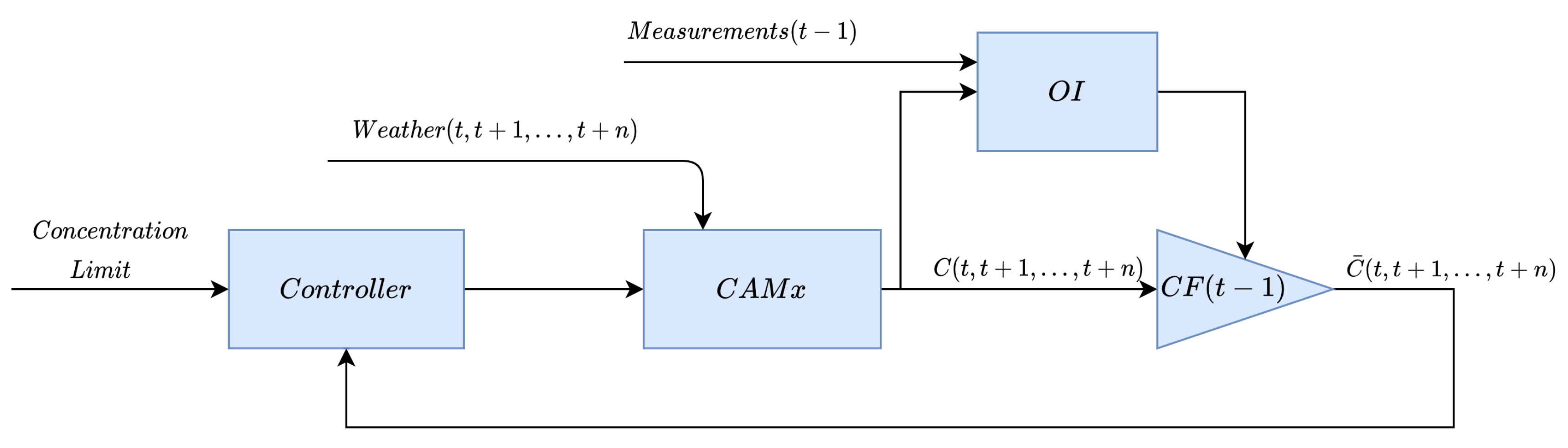
2. Methodology
2.1. Problem Formulation
- is the objective function to be minimized, i.e., the sum of the objective functions V computed for each step. In this work, it includes both an air quality index and a cost index;
- is the air quality model, allowing to estimate the evolution of the concentration of different pollutants in the atmosphere as a function of the concentration values computed at previous steps, the input controlled variable (emissions) and the uncontrolled ones (meteorology);
- is the state of the system, i.e., the concentration of each species in each cell of the computational domain;
- is the control sequence, as defined in Equation (1);
- U is the feasible control set.
2.2. Control Sequence
- Abatement factor: percentage emission reduction resulting from the application of an action on a domain cell. This factor depends on where the measure is applied, due to the presence of different drivers (emission activities) in different locations, i.e., wood burning reduction and traffic limitations do not have the same effect if applied in city centres or rural areas.
- Application map: the area of application of an action. In order to keep considering as a binary value array, if a measure is applied on different areas, it will be considered as two separate measures.
- Cost: implementing an STA has a cost that can be expressed both as a monetary or a social disappointment cost.
- is the emission value of pollutant p at cell d D.
- is the initial condition of the emission value, without the application of any of the abatement measures studied.
- is the effectiveness of the abatement measures applied for the control law , it represents how much the measures manage to reduce the given pollutant p at cell d.
2.3. Objective Function
2.4. Air Quality Forecast
2.5. Optimal Interpolation
- is the background simulated field (first guess), in this case, the output of the deterministic model CAMx.
- is the vector of true values.
- represents the error of the simulated values.
- is the observation vector that contains all the measurements.
- H is a linear operator linking the grid field and the observations, typically bilinear interpolation is applied.
- represents the error of the observations.
- P is the simulation errors covariance matrix.
- R is the observation errors covariance matrix.
- and , thus both errors are unbiased.
- , thus the simulation errors are independent from the measurement ones.
3. Optimization Problem Solution
- to run the deterministic model CAMx is computationally expensive;
- the huge number of input variables and relationships involved in CAMx to describe the phenomena of formation and accumulation of atmospheric pollutants makes the function modelled through the CTM model too complex to be studied;
- the objective of the decision maker in the short-term period is to avoid/limit critical situation, i.e., the situation where the concentration values for a pollutant is higher than a critical threshold (usually defined at the legislative level).
- Forecast Horizon Window: it determines how many steps ahead the pollutant concentrations are forecasted. A wide forecast window will increase the model uncertainty and the computational burden for each cycle. However, abatement measures usually have a higher impact if applied in advance;
- Application Interval Length: this determines for how many days, within the Forecast Horizon, the chosen actions are applied. In other words, it represents the actual control output length and the interval of time between subsequent IAM runs. This variable has a practical limitation, as its minimum value corresponds to running the IAM system and applying the optimal actions within the same day. This is highly unlikely to be obtained in a real life application for any authority. On the other hand, keeping this value as small as possible, allows the system to change the measures selection to cope with new, more accurate forecasts.
- Measure Drop Threshold: This threshold determines the maximum air quality index degradation allowed during the optimization process, with respect to the best index value obtainable with the maximum application of all the measures. Thus, lower values will increase the weight of the air quality objective, higher values, instead, will increase the weight of the cost. For this work this value was set to 1.
- the control law is computed only if the air quality limit value is exceeded within the forecasting horizon window ;
- the control law computation starts with all the actions simultaneously applied for all the application interval length;
- each action is deactivated individually, and the impacts of these individual deactivations are assessed according to the following rules:
- exceedance days should not increase. If the deactivation of an action results in an increase, then the STA cannot be deactivated;
- the worsening of the air quality level, should be less than the value defined by the Measure Drop Threshold. If the worsening is higher, then the measure cannot be deactivated;
- the action with the highest cost among the ones respecting the previous rules is dropped. If two actions have the same cost, then the one with the highest air quality worsening is deactivated.
- the set of the resulting active STA is used as the base case for another iteration in order to deactivate other measures.
- finally, when no deactivation respects the previous control rules, the optimal set of actions is found.
4. Case Study
4.1. Case Study Setup
4.2. Validation of Camx Model for PM Concentration
4.3. Actions
- precursor abatement efficiency;
- application area;
- cost.
- Traffic Limitation/Car Ban: Traffic is among the main pollutant activities in the area, emitting significant quantities of NO through internal combustion, primary PM from brakes and tires abrasion and particle re-suspension. In this short-term case study, traffic measures are applied with a limited time span (down to one day).
- Maximum Speed Reduction: This action, if applied to highways and main streets, proved, in previous studies, to be a viable option to obtain concentration reductions near the streets [43], despite little influence at higher scales.
- Heating Temperature Reduction: one degree reduction of indoor temperature. Even if the reduction factor is small, the area of application allows temperature reduction to cut a significant amount of emissions.
- Wood Burning Limitation in the area under study 98% of domestic heating emissions comes from biomass burning. Long term limitations are already in place, but further emergency limitations are expected to effectively contribute to particulate concentration reductions.
4.4. Objective Function and Control Law Definition
4.5. Results
- Test 1: applies the IAM (with control) with a three day forecast horizon and keeping the application of the resulting measures fixed for the next three days. Optimal interpolation is based on the measurements of the day before the IAM run. This test simulates a situation in which the decision maker cannot change the strategy every day;
- Test 2: applies the daily IAM (with control) with a three day forecast horizon. In this case the pool of measures applied varies every day. This is the standard implementation of the receding horizon technique, but it implies that the decision makers can impose every day different measures to the population. Optimal interpolation is based again on the measurements of the day before each IAM run;
5. Conclusions
- Running the IAM every day increases the computational burden and leaves little notification time for a real world application, but it allows to obtain better results with respect to occasional IAM runs for wider time windows. Further studies should be done in order to determine the best forecast window and running frequency combination to enhance the controller performance.
- PM exceedances forecasting is a challenging problem. Even if the overall performances of the CAMx model are good (in particular in combination with the implemented optimal interpolation technique), little deviations with respect to the measured values can consistently affect the performances, in particular when values are close to the threshold.
- The actions applied in order to reduce particulate matter concentration only over the city of Brescia, also resulted in an air quality improvement for the surrounding areas.
- Further studies should be done in order to add variability to the cost index to take into account the disadvantages arising from last minute notification to the population. This also implies the need of a better model in order to predict further in time.
- Long term actions effects (such as those arising from regional plans) should be included in the problem allowing to evaluate the combined effects with the short term actions selected by the short term IAM.
Author Contributions
Funding
Conflicts of Interest
References
- Landrigan, P.; Fuller, R.; Acosta, N.; Adeyi, O.; Arnold, R.; Basu, N.; Baldé, A.; Bertollini, R.; Bose-O’Reilly, S.; Boufford, J.; et al. The Lancet Commission on pollution and health. Lancet 2018, 391, 462–512. [Google Scholar] [CrossRef] [Green Version]
- Pope, C., III; Dockery, D.; Spengler, J.; Raizenne, M. Respiratory health and PM10 pollution: A daily time series analysis. Am. Rev. Respir. Dis. 1991, 144, 668–674. [Google Scholar] [CrossRef]
- Pope, C., III; Dockery, D. Acute health effects of PM10 pollution on symptomatic and asymptomatic children. Am. Rev. Respir. Dis. 1992, 145, 1123–1128. [Google Scholar] [CrossRef] [PubMed]
- Miranda, A.; Silveira, C.; Ferreira, J.; Monteiro, A.; Lopes, D.; Relvas, H.; Borrego, C.; Roebeling, P. Current air quality plans in Europe designed to support air quality management policies. Atmos. Pollut. Res. 2015, 6, 434–443. [Google Scholar] [CrossRef] [Green Version]
- Manerba, D.; Mansini, R.; Zanotti, R. Attended Home Delivery: Reducing last-mile environmental impact by changing customer habits. IFAC Pap. 2018, 51, 55–60. [Google Scholar] [CrossRef]
- Zhang, M.; Shan, C.; Wang, W.; Pang, J.; Guo, S. Do driving restrictions improve air quality: Take Beijing-Tianjin for example. Sci. Total Environ. 2020, 712, 136408. [Google Scholar] [CrossRef]
- Giannouli, M.; Kalognomou, E.A.; Mellios, G.; Moussiopoulos, N.; Samaras, Z.; Fiala, J. Impact of European emission control strategies on urban and local air quality. Atmos. Environ. 2011, 45, 4753–4762. [Google Scholar] [CrossRef]
- Li, L.; Zheng, Y.; Zheng, S.; Ke, H. The new smart city programme: Evaluating the effect of the internet of energy on air quality in China. Sci. Total Environ. 2020, 714, 136380. [Google Scholar] [CrossRef]
- Turrini, E.; Vlachokostas, C.; Volta, M. Combining a Multi-Objective Approach and Multi-Criteria Decision Analysis to Include the Socio-Economic Dimension in an Air Quality Management Problem. Atmosphere 2019, 10, 381. [Google Scholar] [CrossRef] [Green Version]
- Marques, G.; Pires, I.M.; Miranda, N.; Pitarma, R. Air Quality Monitoring Using Assistive Robots for Ambient Assisted Living and Enhanced Living Environments through Internet of Things. Electronics 2019, 8, 1375. [Google Scholar] [CrossRef] [Green Version]
- Arroyo, P.; Lozano, J.; Suárez, J. Evolution of Wireless Sensor Network for Air Quality Measurements. Electronics 2018, 7, 342. [Google Scholar] [CrossRef] [Green Version]
- Carnevale, C.; Finzi, G.; Pederzoli, A.; Pisoni, E.; Thunis, P.; Turrini, E.; Volta, M. A methodology for the evaluation of re-analyzed PM10 concentration fields: A case study over the PO Valley. Air Qual. Atmos. Health 2015, 8, 533–544. [Google Scholar] [CrossRef]
- Candiani, G.; Carnevale, C.; Finzi, G.; Pisoni, E.; Volta, M. A comparison of reanalysis techniques: Applying optimal interpolation and Ensemble Kalman Filtering to improve air quality monitoring at mesoscale. Sci. Total Environ. 2013, 458–460, 7–14. [Google Scholar] [CrossRef] [PubMed]
- Grivas, G.; Chaloulakou, A. Artificial neural network models for prediction of PM10 hourly concentrations, in the Greater Area of Athens, Greece. Atmos. Environ. 2006, 40, 1216–1229. [Google Scholar] [CrossRef]
- San José, R.; Pérez, J.L.; Morant, J.L.; González, R.M. European operational air quality forecasting system by using MM5–CMAQ–EMIMO tool. Simul. Model. Pract. Theory 2008, 16, 1534–1540. [Google Scholar] [CrossRef]
- Manders, A.; Schaap, M.; Hoogerbrugge, R. Testing the capability of the chemistry transport model LOTOS-EUROS to forecast PM10 levels in the Netherlands. Atmos. Environ. 2009, 43, 4050–4059. [Google Scholar] [CrossRef]
- Carnevale, C.; De Angelis, E.; Finzi, G.; Turrini, E.; Volta, M. An integrated forecasting system for air quality control. In Proceedings of the 2019 18th European Control Conference, ECC 2019, Naples, Italy, 25–28 June 2019; pp. 830–835. [Google Scholar]
- Ou, Y.; Shi, W.; Smith, S.J.; Ledna, C.M.; West, J.J.; Nolte, C.G.; Loughlin, D.H. Estimating environmental co-benefits of U.S. low-carbon pathways using an integrated assessment model with state-level resolution. Appl. Energy 2018, 216, 482–493. [Google Scholar] [CrossRef]
- Qiu, X.; Zhu, Y.; Jang, C.; Lin, C.J.; Wang, S.; Fu, J.; Xie, J.; Wang, J.; Ding, D.; Long, S. Development of an integrated policy making tool for assessing air quality and human health benefits of air pollution control. Front. Environ. Sci. Eng. 2015, 9, 1056–1065. [Google Scholar] [CrossRef]
- Turrini, E.; Carnevale, C.; Finzi, G.; Volta, M. A non-linear optimization programming model for air quality planning including co-benefits for GHG emissions. Sci. Total Environ. 2018, 621, 980–989. [Google Scholar] [CrossRef]
- Carnevale, C.; Ferrari, F.; Guariso, G.; Maffeis, G.; Turrini, E.; Volta, M. Assessing the Economic and Environmental Sustainability of a Regional Air Quality Plan. Sustainability 2018, 10, 3568. [Google Scholar] [CrossRef] [Green Version]
- Gimez Vilchez, J.; Julea, A.; Peduzzi, E.; Pisoni, E.; Krause, J.; Siskos, P.; Thiel, C. Modelling the impacts of EU countries electric car deployment plans on atmospheric emissions and concentrations. Eur. Transp. Res. Rev. 2019, 11, 40. [Google Scholar] [CrossRef]
- Relvas, H.; Miranda, A.; Carnevale, C.; Maffeis, G.; Turrini, E.; Volta, M. Optimal air quality policies and health: A multi-objective nonlinear approach. Environ. Sci. Pollut. Res. 2017, 24, 13687–13699. [Google Scholar] [CrossRef] [PubMed]
- Pisoni, E.; Thunis, P.; Clappier, A. Application of the SHERPA source-receptor relationships, based on the EMEP MSC-W model, for the assessment of air quality policy scenarios. Atmos. Environ. 2019, 4, 100047. [Google Scholar] [CrossRef]
- Thunis, P.; Degraeuwe, B.; Pisoni, E.; Meleux, F.; Clappier, A. Analyzing the efficiency of short-term air quality plans in European cities, using the CHIMERE air quality model. Air Qual. Atmos. Health 2017, 10, 235–248. [Google Scholar] [CrossRef] [PubMed]
- Grune, L.; Pannek, J. Nonlinear Model Predictive Control—Theory and Algorithms; Springer: Berlin/Heidelberg, Germany, 2011. [Google Scholar]
- Ramboll Environment and Health. CAMx User’s Guide Version 6.50; Technical Report; Ramboll Environment and Health: Copenhagen, Denmark, April 2018. [Google Scholar]
- Carnevale, C.; Finzi, G.; Guariso, G.; Pisoni, E.; Volta, M. Surrogate models to compute optimal air quality planning policies at a regional scale. Environ. Model. Softw. 2012, 34, 44–50. [Google Scholar] [CrossRef]
- Carnevale, C.; Pisoni, E.; Volta, M. Formalizing and solving the PM10 control problem. In Proceedings of the 17th World Congress, the International Federation of Automatic Control, Seoul, Korea, 6–11 July 2008. [Google Scholar]
- Whitten, G.Z.; Heo, G.; Kimura, Y.; McDonald-Buller, E.; Allen, D.T.; Carter, W.P.; Yarwood, G. A new condensed toluene mechanism for Carbon Bond: CB05-TU. Atmos. Environ. 2010, 44, 5346–5355. [Google Scholar] [CrossRef]
- Yarwood, G.; Rao, S.; Yocke, M.; Whitten, G. Updates to the Carbon Bond Chemical Mechanism: CB05; Final Report; US-EPA: Washington, DC, USA, 2005.
- Bott, A. Improving the time-splitting errors of one-dimensional advection schemes in multidimensional applications. Atmos. Res. 2010, 97, 619–631. [Google Scholar] [CrossRef]
- Wesely, M.; Hicks, B. A review of the current status of knowledge on dry deposition. Atmos. Environ. 2000, 34, 2261–2282. [Google Scholar] [CrossRef]
- Hertel, O.; Berkowicz, R.; Christensen, J.; Hov, Ã. Test of two numerical schemes for use in atmospheric transport-chemistry models. Atmos. Environ. Part Gen. Top. 1993, 27, 2591–2611. [Google Scholar] [CrossRef]
- Fountoukis, C.; Nenes, A. ISORROPIAII: A computationally efficient thermodynamic equilibrium model for K+-Ca2+-Mg2+-NH4 +-Na+-SO42-NO3-Cl-H2O aerosols. Atmos. Chem. Phys. 2007, 7, 4639–4659. [Google Scholar] [CrossRef] [Green Version]
- Strader, R.; Lurmann, F.; Pandis, S. Evaluation of secondary organic aerosol formation in winter. Atmos. Environ. 1999, 33, 4849–4863. [Google Scholar] [CrossRef]
- Carnevale, C.; Angelis, E.; Finzi, G.; Pederzoli, A.; Turrini, E.; Volta, M. A non linear model approach to define priority for air quality control. IFAC Pap. 2018, 51, 210–215. [Google Scholar] [CrossRef]
- Candiani, G.; Carnevale, C.; Filisina, V.; Finzi, G.; Pisoni, E.; Volta, M. Optimal interpolation to re-analyse PM10 concentration modelling simulations. In Proceedings of the 48th IEEE Conference on Decision and Control (CDC) Held Jointly with 2009 28th Chinese Control Conference, Shanghai, China, 15–18 December 2009; pp. 1794–1799. [Google Scholar]
- Carnevale, C.; Douros, J.; Finzi, G.; Graff, A.; Guariso, G.; Nahorski, Z.; Pisoni, E.; Ponche, J.L.; Real, E.; Turrini, E.; et al. Uncertainty evaluation in air quality planning decisions: A case study for Northern Italy. Environ. Sci. Policy 2016, 65, 39–47. [Google Scholar] [CrossRef]
- Skamarock, W.C.; Klemp, J.; Dudhia, J.; Gill, D.O.; Barker, D.M.; Duda, M.G.; Huang, X.Y.; Wang, W.; Powers, J.G. A Description of the Advanced Research WRF Version 3; Note NCAR/TN-475+STR; NCAR: Boulder, CO, USA, 2008. [Google Scholar]
- ARPA Lombardia. INEMAR—Lombardy Region Emission Inventory. 2011. Available online: http://www.inemar.eu (accessed on 21 January 2016).
- Emmons, L.K.; Walters, S.; Hess, P.G.; Lamarque, J.F.; Pfister, G.G.; Fillmore, D.; Granier, C.; Guenther, A.; Kinnison, D.; Laepple, T.; et al. Description and evaluation of the Model for Ozone and Related chemical Tracers, version 4 (MOZART-4). Geosci. Model Dev. 2010, 3, 43–67. [Google Scholar] [CrossRef] [Green Version]
- Hodges, N.; Obzynska, D.J.; Lad, D.C.; Swaton, R. Air Quality Management Guidebook. Technical Report, Citeair—INTERREG 3C Project. 2005. Available online: http://citeair.rec.org/downloads/Products/AirQualityManagement.pdf (accessed on 2 May 2020).


| Feature | Options |
|---|---|
| Chemical Mechanism | CB05 [30,31] |
| Advection Solver | BOTT [32] |
| Drydep Model | WESELY [33] |
| Chemistry Solver | EBI [34] |
| Aerosol Approach | CF [27] |
| Inorganic Thermodynamic module | ISORROPIA [35] |
| Organic Aerosol module | SOAP [36] |
| Action | Zone | PM Reduction | NO Reduction | Cost |
|---|---|---|---|---|
| Traffic Limitation | 1 | 42% | 51% | 2 |
| Traffic Limitation | 2 | 25% | 52% | 3 |
| Traffic Limitation | 3 | 25% | 52% | 5 |
| Speed Reduction | 4 | 23% | 5% | 2 |
| Reduce Heating | 3 | 5% | 5% | 2 |
| Wood Burning Limitation | 1 | 30% | 4% | 2 |
| Wood Burning Limitation | 2 | 50% | 7% | 3 |
| Wood Burning Limitation | 3 | 50% | 7% | 4 |
| Test | Exceedances | Cost | PM |
|---|---|---|---|
| Base Case | 26 | 0 | 77.5 |
| Test 1 | 24 | 268 | 69.0 |
| Test 2 | 23 | 253 | 69.0 |
| Test Max | 21 | 351 | 67.3 |
© 2020 by the authors. Licensee MDPI, Basel, Switzerland. This article is an open access article distributed under the terms and conditions of the Creative Commons Attribution (CC BY) license (http://creativecommons.org/licenses/by/4.0/).
Share and Cite
Carnevale, C.; De Angelis, E.; Tagliani, F.L.; Turrini, E.; Volta, M. A Short-Term Air Quality Control for PM10 Levels. Electronics 2020, 9, 1409. https://doi.org/10.3390/electronics9091409
Carnevale C, De Angelis E, Tagliani FL, Turrini E, Volta M. A Short-Term Air Quality Control for PM10 Levels. Electronics. 2020; 9(9):1409. https://doi.org/10.3390/electronics9091409
Chicago/Turabian StyleCarnevale, Claudio, Elena De Angelis, Franco Luis Tagliani, Enrico Turrini, and Marialuisa Volta. 2020. "A Short-Term Air Quality Control for PM10 Levels" Electronics 9, no. 9: 1409. https://doi.org/10.3390/electronics9091409