Abstract
The weapon-target assignment problem is a crucial decision support in a Command and Control system. As a typical operational scenario, the major asset-based dynamic weapon target assignment (A-DWTA) models and solving algorithms are challenging to reflect the actual requirement of decision maker. Deriving from the “shoot–look–shoot” principle, an “observe–orient–decide–act” loop model for A-DWTA (OODA/A-DWTA) is established. Focus on the decide phase of the OODA/A-DWTA loop, a novel A-DWTA model, which is based on the receding horizon decomposition strategy (A-DWTA/RH), is established. To solve the A-DWTA/RH efficiently, a heuristic algorithm based on statistical marginal return (HA-SMR) is designed, which proposes a reverse hierarchical idea of “asset value-target selected-weapon decision.” Experimental results show that HA-SMR solving A-DWTA/RH has advantages of real-time and robustness. The obtained decision plan can fulfill the operational mission in the fewer stages and the “radical-conservative” degree can be adjusted adaptively by parameters.
1. Introduction
Weapon target assignment (WTA), which is also known as Weapon Allocation or Weapon Assignment (WA), refers to the reactive assignment of defensive weapons to counter identified threats [1]. With the development of advanced weapons and combat theory, it is difficult for human decision-makers to counter the fire allocation problem effectively in the complex operational environment [2]. WTA is studied as a critical problem in an intelligent decision support system in order to reduce the decision pressure of human decision-makers or replace them.
The WTA problem was first introduced by Manne in 1959 [3]. In the following decades, various types of WTA problems have evolved. From the decision process, the WTA problem can be divided into static WTA (SWTA) [4] and dynamic WTA (DWTA) [5,6]. The difference between SWTA and DWTA is whether the time is considered as a dimension. SWTA launches weapons in a salvo to maximize operational effectiveness. DWTA assigns the sequence of weapons for the equilibrium plan during multi-stage [7]. According to the operational mission, there are mainly target-based WTA (T-WTA) [8], asset-based WTA (A-WTA) [9] and sensor-WTA (S-WTA) [10,11] model. The T-WTA model adopts the kill effectiveness of weapons against targets as the optimization objective. The purpose of the A-WTA problem is to maximize the survival values of own assets. S-WTA considers the collaborations between sensors and weapons. This paper focuses on the A-DWTA problem.
A-DWTA problem is a more complex WTA problem, combining the characteristics of DWTA and A-WTA problems, and most WTA models can be seen as a special case of A-DWTA model. For example, the DWTA model can be considered as the zero-asset value of the A-DWTA model, and the A-WTA model can be considered as the one-stage model of the A-DWTA. Compared with the other WTA problems, the A-DWTA problem is less studied and the research frameworks are different. In the early research, a two-stage A-DWTA model is presented, which considers the dynamic as the repetition of the current stage and next stage. The defense is allowed to observe the outcomes of all engagement of the previous time stage before assigning and committing weapons for the present stage [12,13]. The decision variable of the two-stage model is the number of weapons assigned to the defense of assets, therefore this model has the assumption that the kill probability of a weapon-target pair depends solely on the asset to which the target is aimed [14,15]. Although the two-stage model considered the case of two-stage DWTA problem, the referenced conclusion can be extended to the multi-stage model [16,17,18]. With the advancement of optimization theory, the multi-stage model gradually becomes the major of WTA research problem [19]. The objective of the multi-stage model is to maximize the operational effectiveness from the current stage to the predetermined end stage, and the number and types of incoming targets of the remaining stages are known as a probability distribution.
The WTA problem is proved to be NP-complete, and the objective function is convex [20]. The exact algorithms solving the WTA model have a “dimension explosion” dilemma, which does not satisfy the real-time requirements in practical applications [21,22]. Hence, the alternate approaches, such as model transformation, heuristics algorithm, are studied to approximate the optimal solution [23,24,25]. The swarm intelligence algorithm, which is widely used to solve WTA models, has fewer limitations on constraints, and the computational complexity is less sensitive to the problem scale [26,27]. For example, Chen et al. [28] investigated the performance of three evolutionary algorithms, solving the proposed A-DWTA model. Chang et al. [29] put forward an improved artificial bee colony algorithm based on the ranking selection and elite guidance. Wang [30] designed a discrete particle swarm algorithm based on the intuitionistic fuzzy entropy. Lai and Wu [31] proposed an improved simplified swarm optimization with deterministic initialization and target exchange scheme. However, the population-based random search mechanism lacks rigorous theoretical proofs in terms of convergence. In recent years, researches have introduced heuristic information based on domain knowledge into the weapon-target assignment [24,32,33,34]. Domain knowledge generally comes from expert knowledge or empirical rules, and heuristic information based on domain knowledge construction can guide algorithms to perform the deterministic search, which can quickly obtain feasible near-optimal solutions. For example, Ahuja R K et al. [35] calculated the transfer return of weapon nodes and used it as heuristic information to optimize the initial solution obtained by the deterministic algorithm. Lee et al. [36] proposed the weapon-priority factor to obtain the good gene of a genetic algorithm. Xin et al. proposed two tabu search algorithms integrating the virtual permutation and local search to solve the A-DWTA problem, and [37] took the “weapon-target-stage” benefits in the A-DWTA model as heuristic information and distributed the more benefits in turn according to the principle of maximizing weapon killing efficiency. Leboucher et al. presented a dynamic weapon target assignment for area air defense [38], and proposed a multi-objective optimization method based on the evolutionary game theory to solve the A-DWTA problem, which has the advantage of being real-time [39]. Li et al. [40,41,42,43] investigated three multi-objective optimizers of DMOEA-εC, NSGA-II, and MOEA/D-AWA on solving the multi-stage DWTA problem. Mei et al. [44] proposed a heuristic algorithm, which is derived from receding horizon control, to solve the DWTA problem. Chang [29] presented the target-priority factor with a random sequence and Cannikin Law to improve the initial population.
The objectives of the major A-DWTA models are derived from the classic static WTA model and are formulated as the asset value expectation on whole stages. After the multi-stage process of A-DWTA is over, the whole-stage return can indeed evaluate the decision-making performance. However, in the actual operational process, the C2 system makes it challenging to use the global optimization goal as the decision metric of the current stage. There are three main reasons: (1) when calculating the global return, the variables of the subsequent stages can only be described by the probability distribution. Hence the farther prediction from the current stage, the lower the accuracy and real-time performance. (2) Due to the uncertainty of multi-stage evolution, the number of offensive and defensive stages is usually set artificially. The operational experience shows that both sides pursue killing targets in as few stages as possible and ending the combat quickly, so the number of stages should also be one optimization goal. (3) Under the premise that the number of stages can not be determined, the offensive and defensive parties’ primary operational goal is to kill the target efficiently and high cost–effectively in the near stage. Therefore, the decision-maker usually only considers the assignment return of limited stages, rather than the overall stages. In the DWTA problem, the consensus is that the tactical operation should follow the “shoot–look–shoot” strategy [5,45]; that is, the current stage k decides the shooting plan by observing the situation after the shoot of stage , which is a typical Markov Decision Process (MDP) [46]. The “look” and “shoot” phases correspond to the “observe” and “act” phases of the known “observe–orient–decide–act” (OODA) loop. Hence ,the A-DWTA model should be adequately described as an OODA loop system.
Optimizing the objective (21) also faces the following challenges: (1) the decision space is difficult to obtain the optimal global solution of the entire confrontation process while satisfying real-time performance. Assuming that the initial number of weapons is m, the number of targets is m, and there are decision-making stages, then the search space scale of the dynamic weapon-target allocation problem is at least . It is difficult to get the theoretical optimal solution for the medium and large-scale weapon-target allocation problem. (2) The uncertainty of multi-stage prediction. Decision-makers can only observe the system status of the current stage, such as target survival, asset survival, and weapon-target attack conditions. The certainty of the prediction information in the subsequent stages decreases with the extrapolation of the prediction horizon. Therefore, it is hard to achieve multi-stage global optimization by predicting system evolution.
Motivated by the above analysis, we described the OODA/A-DWTA loop system, and decomposed the A-DWTA model by receding horizon strategy (A-DWTA/RH). Then, a heuristic algorithm based on the statistical marginal return (HA-SMR) is proposed to obtain the optimal plan for a decision-maker. The contributions of this paper are described as follows:
- An OODA/A-DWTA loop model is established for supporting the following A-DWTA decision model and solving algorithm.
- To reflect the actual operational requirement, an A-DWTA decision model based on the receding horizon strategy is presented. The “radical–conservative” degree of the obtained plan, which relates to the number of decision stages, can be adaptively adjusted by the model parameter.
- A heuristic algorithm based on statistical marginal return is proposed to solve the A-DWTA model, which has the advantage of robust and real-time. The extensive experiments demonstrate the effectiveness of the proposed approaches.
The rest of this paper is organized as follows. Section 2 gives our motivations and formulates the OODA/A-DWTA loop model. Section 3 formulates the objective and constraints of the A-DWTA decision model. Section 4 presents the proposed HA-SMR for the A-DWTA model. Section 5 verifies the proposed HA-SMR solving the A-DWTA problem by experimental studies. The conclusion is finally summarized in Section 6.
2. Ooda/A-Dwta Loop Model
The OODA loop theory was put forward by John Boyd in the 1970s, and his theoretical viewpoint is that the execution process of a fire strike can be divided into the observe–orient–decide–act cycle. In the conflict, the party who completes the OODA loop faster has the advantage. Therefore, both sides’ antagonistic goal is to accelerate their own OODA cycle, cut off, or delay the enemy OODA cycle process. After half a century of testing, the OODA loop theory has been widely used in military, economic warfare, competitive sports, and other fields.
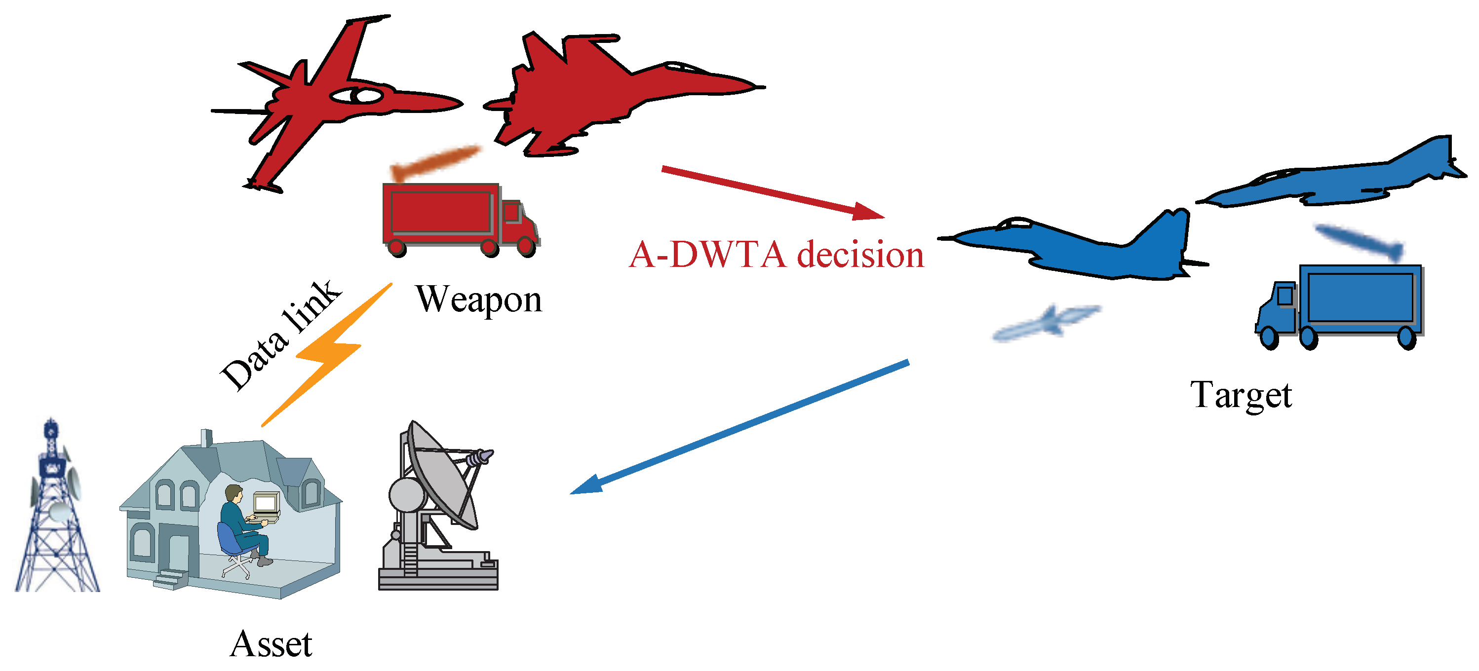
The operational scenario of A-DWTA is: enemy units launch an attack to destroy the assets with military value but no defensive ability, such as military installations, personnel gathering placing, command and control nodes, weapons warehouses and ports. At this time, the defense unit with combat ability is the decision-maker and is to maximize the assets’ survival value in multiple attack and defense stages by allocating weapon resources to kill the enemy targets, as shown in Figure 1.
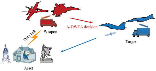
Figure 1.
Schematic diagram of the asset-based weapon target assignment (A-DWTA) scenario.
The A-DWTA problem based on the “shoot–look–shoot” mechanism conforms to the typical OODA loop theory. In the observe phase, the decision-maker updates the external information (target state, asset state) of the current stage. In the orient phase, the state information collected in the observation phase is decomposed and reconstructed, such as the threat assessment based on the target track information, the identification of the attack intention of the targets against assets, the feasibility of a weapon attacking a target, and the determination of attack request. If the termination conditions are met, the weapon system is guided to exit the operational environment, otherwise continue to execute the OODA loop. In the decide phase, the specific combat requirements are converted into objective functions, and the solution is solved according to the designed weapon-target allocation algorithm. In the act phase, execute the weapon-target assignment plan given in the decide phase, update weapon state information, and evaluate the damaging effect of targets and the value of assets. A diagram of the OODA/A-DWTA loop model is shown in Figure 2. The notation employed in the context is listed in Table 1.

Figure 2.
Diagram of the observe–orient–decide–act (OODA)/asset-based dynamic weapon target assignment (A-DWTA) loop model.

Table 1.
Notation declaration.
2.1. Observe Phase
In the OODA/A-DWTA loop, the observation model describes the survival state of assets and the damage state of targets at the current stage under the uncertain battlefield environment.
- (1)
- Target state observation. Let the current stage be s, and the target observed state is the actual survival state of targets after the act phase of stage . Therefore, the observed target state at stage s should follow the Bernoulli distribution about the target survival probability at stage , namely ∼:where indicates that the observed state of the target j in observation phase is damaged; conversely, represents target j as a threat target in observation phase; is the target survival probability expectation after the end of stage , which is given in the damage assessment of the act phase.
- (2)
- Asset state observation. Similarly, the asset observed state of stage s follows the Bernoulli distribution of the asset survival probability expectation of stage . The asset survival probability expectation is related to the target survival probability expectation in the act phase of stage , and the target observed state can be obtained in the stage s. Therefore, in the observation model of OODA/A-DWTA, the asset survival probability expectation of stage is modeled as the posterior conditional probability of the target observed state of stage s:
The asset observed state follows ∼:
where represents that the observed state of asset k at stage s is survival; conversely, represents that the observed state of asset k is destroyed.
2.2. Orient Phase
In the OODA/A-DWTA loop, the orient model is used to determine the attack request, and update the target-asset attack intention, weapon–target attack condition by the observation information.
- (1)
- Attack request determination. When any of the following conditions are met, the OODA/A-DWTA loop terminates, otherwise initiates an attack request and enters the decide phase: (a) all assets are destroyed, , where is the l1-norm; (b) all targets are damaged, ; (c) no available weapon, . So the termination condition of OODA/A-DWTA is .
- (2)
- Target–asset attack intention. In actual combat, the identification of enemy target’s attack intention requires the analysis of target altitude, distance, speed, acceleration, heading angle, azimuth, fire control radar state, maneuver type, and is predicted by domain knowledge. WTA research’s focus lies in the decision model and algorithm of the command and control layer, not the methods of intention recognition. Hence we simplify the target-asset intention matrix to describe the enemy targets’ attack state of each stage. represents that the attack intention of target j against asset k is not recognized at stage s. Otherwise, it represents that target j against asset k, and the destroy probability is .
- (3)
- Weapon–target attack condition. The condition of weapon–target attack is mainly determined by whether the time window of the fire control launch is satisfied. In DWTA, as the offensive and defensive stages recurse, the weapons that meet the attack conditions usually decrease. We introduce the lethality matrix and feasibility matrix to describe the weapon-target attack condition of each stage, where represents the destroy probability of weapon i against target j; indicates that weapon i meets the attack condition of intercepting target j, otherwise .
2.3. Decide Phase
As the critical issue of the OODA/A-DWTA loop, the decide model aims to obtain the optimal weapon-target assignment under the current situation and maximize the survival value expectation of assets.
where is the objective function of the A-DWTA decision model, which directly reflects the operational requirement of C2 system. The solving algorithm of Formula (4) reflects the intelligent degree of weapon-target assignment. As the focus of this paper, the A-DWTA decision model will be studied in detail in the next section.
2.4. Act Phase
According to the obtained weapons-target assignment at the current stage, the act model needs to carry out weapon states update, target damage assessment, and asset survival value assessment.
- (1)
- Weapon state update. After acting the weapon allocation plan, the current stage’s weapon state are determined by the previous stage’s weapon states and the current stage’s decision plan .where denotes weapon i is not available at stage s, otherwise .
- (2)
- Target damage assessment. The target survival probability is mainly determined by the target state, the weapon–target kill probability and the decision plan at current stage.where (6), . If and only if , that is, the target j is confirmed as damaged by the observe phase of the stage s, ; if and only if and , that is, no weapon is not assigned to the target j with threat capability, .
- (3)
- Asset damage assessment. The asset survival value expectation of stage s is related to the asset value and the asset survival probability expectation in the act phase of stage s. In the act model of OODA/A-DWTA, the asset survival probability expectation of stage s is modelled as the conditional probability under the target survival probabilitywhere the term represents the damage probability of target j attacking asset k in the act phase of stage s. The asset survival value expectation is evaluated aswhere . If and only if , that is, the asset k is confirmed as destroyed by the observe phase of the stage s, ; if and only if and , that is, no target has attack intention to the target j, .
In summary, the model of OODA/A-DWTA loop model is
3. A-Dwta/Rh Formulation
In the A-DWTA decision model, it is assumed that there are stages of attack and defense decision-making before the enemy targets are annihilated, or assets are destroyed. In stage s, the problem variables are the destroy effectiveness of enemy targets against assets obtained by threat assessment; the survival value of assets; the defensive effectiveness of weapons against targets and the attack constraints of weapon–target. The output variable is the defense decision matrix . The research goal of the A-DWTA problem is to solve the decision model through algorithms under the current situation , obtain an optimal firepower decision plan , and maximize the effectiveness of reducing enemy targets’ threat to assets.
where the design of the objective function F directly reflects the operational purpose of the command and control system, and the constraints C reflect the battlefield environment. The solving algorithm directly reflects the reasonable degree of firepower decision.
To solve the problem that the standard A-DWTA model pursues the theoretical optimal solution in mathematics and is not tightly integrated with the operational requirements, this section establishes a two-stage A-DWTA model based on the Receding Horizon Strategy (A-DWTA/RH).
3.1. Objective Building
The major objective function of A-DWTA model is derived from the classic static WTA model, and is formulated as the sum of the asset value expectation at each stage, such as
where is the maximum number of decision stages; decision set is the global decision sequence starting from the current stage t, where is the local decision of stage s.
For solving the problem (11), the related algorithms are to set the maximum stages , predict the targets and assets status of all subsequent stages at the current stage, search the current global optimal solution for stage one to . In response to this problem, we believe that the maximum number of stages is one of the most crucial algorithm metrics in the A-DWTA problem. The primary task of decision-makers is still to kill the targets efficiently and protect assets from damage cost-effectively in the fewest stages. Secondly, considering the uncertainty of weapons killing targets, it is still necessary to ensure the remaining weapons’ ability to counter survival targets in subsequent stages. Following the above idea, we propose a two-stage A-DWTA model based on the receding horizon strategy. The design of the objective function follows two points: (1) from the perspective of the decision-maker, it should first ensure the efficient and cost-effective killing of targets at the current stage to achieve the purpose of protecting our assets. (2) Assuming the targets have not been killed after the act of the current stage, the remaining weapons should have sufficient countermeasures against the enemy target. In summary, the objective function of the A-DWTA/RH model is composed of two parts. The first part is the direct income expectation of weapons killing targets in the current stage, and the second part is the prediction return of the remaining weapons against the undamaged target in the next stage, as shown
where represents the absolute return expectation of the decision variable b at the current stage; represents the threat return of the remaining weapons to the target under the prediction situation of the stage , and denotes the remaining available weapon set after the action process of stage s. and respectively represent the target survival probability and asset survival probability under the situation and the decision variable , calculated according to the system state transfer Equation (9). is a weight parameter reflecting the decision maker’s preference for and in the objective function. and are normalized.
3.1.1. Absolute Return Expectation at the Current Stage
The absolute return expectation at the current stage can be expressed by the combat effectiveness of the used weapons at the current stage: the survival value expectation of assets under the weapon-target assignment scheme. Let the current stage be the stage s and the decision variable is , then the normalized combat effectiveness of the current stage is
Substitute the Formula (6) into the above formula to get
3.1.2. Return Evaluation of Remaining Weapons on Prediction Situation
Since the current stage cannot obtain the situation information such as the weapon/target/asset status and target attack intention of the next stage, it is necessary to design the return evaluation method of combat mission under the prediction situation. The designed evaluation method is: due to the event “weapons attack the target,” the threat of the target to the asset will be attenuated, and the value expectation of the asset will rise. Therefore, according to the state distribution of the situation information in the next stage, the value expectation of assets under the situation of “threatening target–surviving asset” is calculated first. Then the value expectation under the situation of “surplus weapon–threatening target–surviving asset” is calculated. The difference between the two value expectation can be used as the return expectation of remaining weapons in the prediction situation.
Based on the above ideas, after the weapon-target assignment plan is implemented at the stage s, the OODA/A-DWTA loop established in Section 2 gives: the weapon state is , the target state is subject to ∼, and the asset state is subject to (6). The return expectation of each “remaining weapon–threat target-survival asset” subject to the above distribution can be used as the return of the remaining weapon in the prediction situation. First, regardless of weapons , the prediction threat of targets to assets can be evaluated as:
From the above formula, considering the damage of weapons on targets , the prediction threat to assets can be evaluated as
3.2. Constraints
In the A-DWTA model, the necessary mathematical constraints include 0–1 integer constraints of decision variables, and total constraints of weapons, as shown below:
Besides, model constraints can be designed according to specific DWTA models. Commonly used model constraints include multi-target attack constraints and weapon consumption constraints on single-target.
where the first term is the multi-target attack constraint, limiting the number of targets that one weapon can attack at one stage. In the coding of WTA models, the weapon platform is usually disassembled into single-weapon, that is, . The second item is the weapon consumption constraint on single-target, which is the upper limit of the number of weapons allocated to one target at one stage. This paper considers that the motivation of constraint (19) is to control the consumption of weapons at each stage, prevent excessive consumption of weapons and the DWTA model degenerating into the SWTA model. In the auxiliary decision-making system, this constraint is not the operational index that the decision-maker concentrates on. Furthermore, the artificial setting of itself adds an extra burden of decision-making and cannot directly reflect the improvement of combat effectiveness.
To quantify the cost-effectiveness ratio of the decision plan more accurately and reduce the burden on decision-makers, we convert the constraints (19) into the gradient limit of target survival value based on the characteristics of the weapon consumption characteristic curve. The attenuation of firepower return is employed as constraint metric
where is the threshold parameter of weapon consumption. In summary, the proposed A-DWTA/RH model and constraints are
4. Ha-Smr Algorithm
This section analyzes the limitations of the heuristic information commonly used in the current WTA algorithms, proposes heuristic information based on statistical marginal return, and designs an A-DWTA solving algorithm based on this heuristic information.
4.1. Algorithm Framework
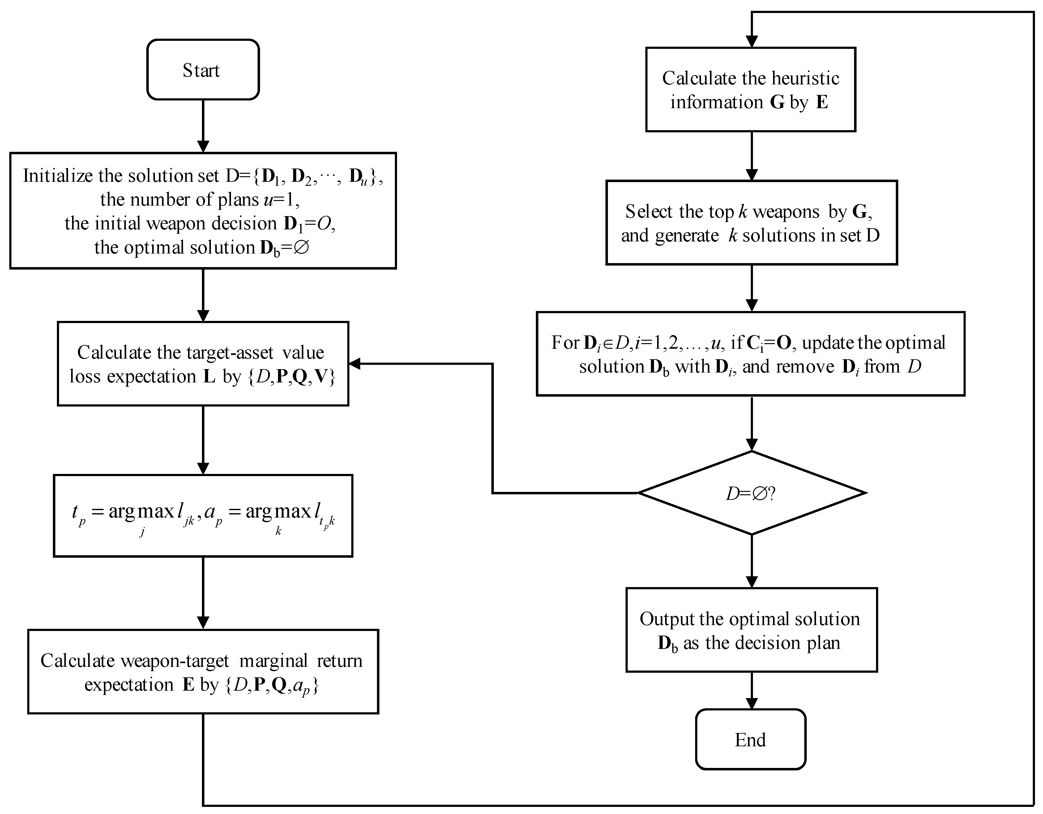
Disassembling the offensive and defensive relationship of the A-DWTA/RH decision model shows that there are two types of decision plans: (1) target–asset attack plan; (2) weapon–target assignment plan. It can be seen that the return flow of the objective function of the A-DWTA/RH model is “weapon–target–asset.” Therefore, the algorithm proposed in this paper is to perform the reverse hierarchical way of “asset value–target selected–weapon decision.” First, based on the perspective of asset defense, calculate the value loss expectation of each asset according to the current weapon-target plan, target–asset intention, and target–asset destroy probability, then select the resource with the maximal value loss expectation as the priority defense asset. Secondly, calculate the value loss expectation caused by each target attacking the priority defense asset, and select the target corresponding to the maximum value as the priority attack target. Finally, the priority weapon is solved for by heuristic information. The decision plan is updated, and the weapon is removed from the set of available weapons. Return to update the state of the decision-making system and repeat the above operations until the algorithm meets the termination condition. In the above iterative process, the diversity of the decision set and the algorithm’s real-time performance are maintained by the objective function.
The main loop of MOEA-CMWTA is outlined in Algorithm 1. The flow diagram of HA-SMR is shown in Figure 3.
| Algorithm 1. Main loop of heuristic algorithm based on statistical marginal return (HA-SMR). |
|
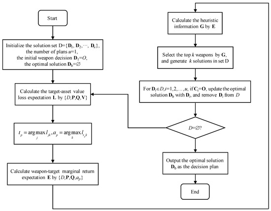
Figure 3.
Flow diagram of heuristic algorithm based on statistical marginal return.
4.1.1. Priority of Target and Asset
To facilitate the understanding of the algorithm proposed in this chapter, first define the key variable between the “weapon–target” and “target–asset” situations in the A-DWTA model: the equivalent conditional kill probability.
Definition 1.
(Equivalent Conditional Kill Probability). In the A-DWTA model, considering the determined weapon-target assignment plan, the expected kill probability of targets against assets under the “weapon–target–asset” situation is defined as equivalent conditional kill probability.
First, let the current weapon–target decision matrix be , the target–asset destroy matrix be , and the equivalent kill condition probability matrix of weapon-target-asset be
Second, calculate the target-asset loss value expectation matrix based on the target-asset equivalent condition damage probability and the asset survival value
where . At this time, the value of the element represents the loss value expectation of the two-tuple “target j–asset k” under the current decision matrix . According to the maximum marginal return strategy, the maximum element in the loss value expectation matrix D is extracted to determine the priority defense asset A, and then the priority attack target B is selected, namely
4.1.2. Weapon–Target Marginal Return Expectation
Theorem 1.
Under the current decision D and situation , the weapon-target marginal return expectation matrix of the A-DWTA model is
where represents the marginal return expectation of the value of asset generated by weapon i attacking target j, and asset is the attack intention of target j; denotes the equivalent kill condition probability of target h against asset k.
Proof of Theorem 1.
Under the current decision and situation , the target–asset equivalent conditional killing probability is , and the value expectation of each asset is :
Take target with attack intention to asset , i.e., , for example. If weapon is available and assign , then the equivalent conditional killing probability of target to asset under triad is
Then the value expectation of asset is
Difference Formulas (28) and (29) shows that the transfer function from weapon against target to the marginal return expectation of asset is
Substitute the equivalent conditional kill probability d of Formula (23) into the above formula. Without loss of generality, the weapon–target marginal return expectation matrix is
□
According to the above proof, it can be seen that the matrix has been constrained, and when the following three situations occur: (1) weapon i is unavailable; (2) target j has been destroyed; (3) weapon i is available, and target j is not damaged, but the pair does not meet the attackable condition, .
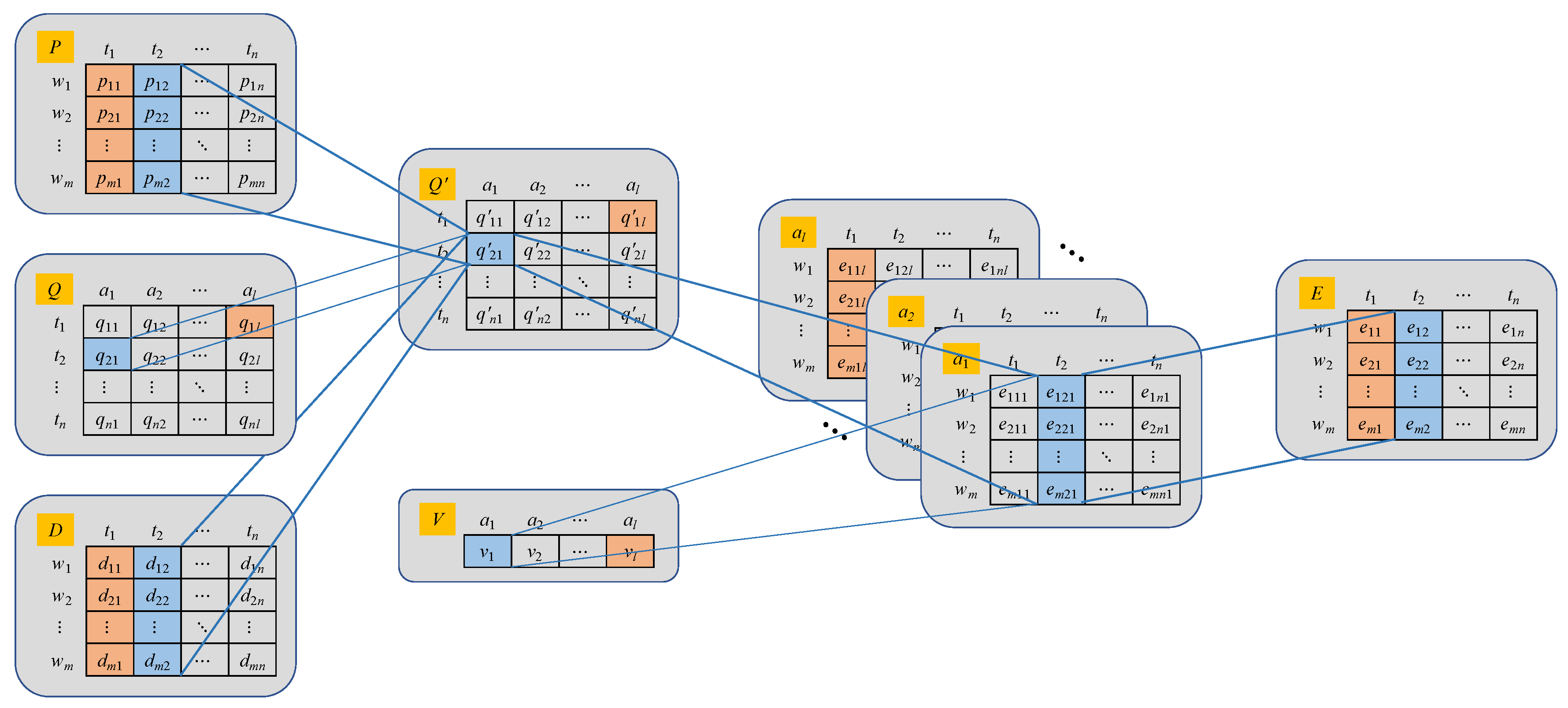
The information flow diagram of the calculation of the weapon–target marginal return expectation is shown in Figure 4.
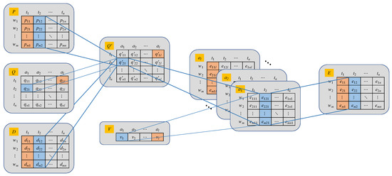
Figure 4.
Information flow of the calculation of weapon–target marginal return expectation.
4.2. Heuristic Information Design
Under the reverse hierarchical solution strategy proposed above, the A-DWTA model has been transformed into a weapon selection problem similar to the SWTA model. In the WTA problem, the heuristic information of weapon selection is usually based on the construction of combat efficiency maximized from the current perspective [10,29,36]. First, calculate the comprehensive kill efficiency matrix based on the target value and the kill probability matrix .
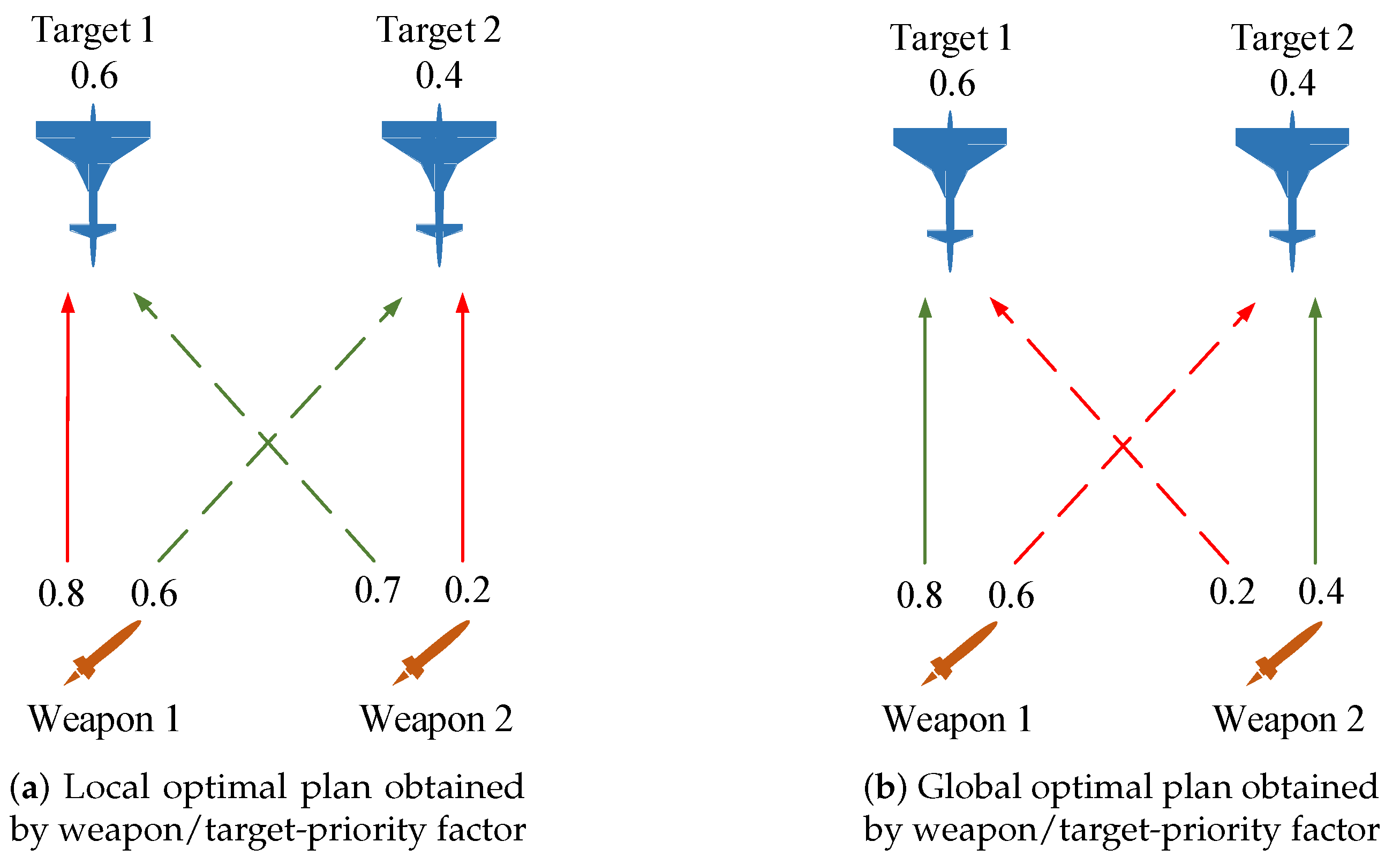
According to different decision-making perspectives, the heuristic information based on killing effectiveness can be roughly divided into weapon–priority heuristic information and target–priority heuristic information. Weapon/target–priority heuristic information is widely used in large-scale WTA algorithms, which can improve the real-time performance and quickly obtain feasible solutions. However, the following analysis shows that the heuristic information based on the local perspective can easily make the search algorithm fall into the local optimal solution. Taking the 2*2 scale as an example, in Figure 5a, according to the decision process based on weapon-priority heuristic information, the return expectation of weapon 1 against target 1 is 0.8 × 0.6 = 0.48, and the return expectation of weapon 1 against target 2 is 0.6 × 0.4 = 0.24. The principle of maximizing return will assign weapon 1 to target 1, and the value expectation of target 1 is updated to 0.6 × (1 − 0.8) = 0.12. Continue to execute the allocation of weapon 2. Return the expectation of weapon 2 attacking target 1 is 0.2 × 0.12 = 0.024, and the return expectation of weapon 2 attacking target 2 is 0.4 × 0.4 = 0.16. Therefore, the allocation scheme of will be generated. Similarly, the same local optimal scheme can be obtained by using the target–priority heuristic information. However, the optimal scheme can be known through enumeration. In Figure 5b, the global optimal allocation scheme can be obtained by using the weapon/target-priority heuristic information.
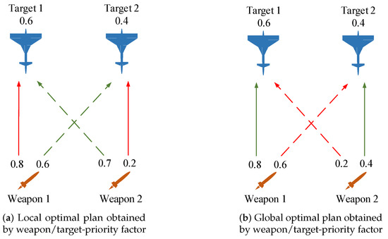
Figure 5.
Defects based on weapon/target priority heuristic information.
In Figure 5a, the weapon/target priority heuristic information makes the decision plan fall into local optimal, while in Figure 5b, the weapons/target priority heuristic information leads to the global optimal plan. By analyzing the internal reasons and mechanisms, the following inference is presented: heuristic information based on statistical marginal return can better overcome local optimal than heuristic information that maximizes marginal return from a single perspective.
The main reason why the maximum marginal return heuristic information easily falls into a locally optimal solution is that, in the case of certain coupling of weapon–target killing efficiency, the weapon-target assignment from the maximum marginal return is terrible under the global perspective. For example, if the killing effect of weapon against other targets is much smaller than that of the target , the maximum marginal benefit heuristic information will execute the decision , so that the threat weight of target j will decay rapidly. Then, the marginal benefit of the remaining weapon attacking target is minimal and is usually allocated to the other targets . If weapon has a better killing effect on the other targets , and the remaining weapons have a better killing effect on target , the decision has fallen into a terrible local optimal solution.
In order to overcome the above coupling mechanism, this paper constructs heuristic information based on statistical marginal return: if a weapon has high killing efficiency against a few targets and low killing efficiency against the other targets, it is considered to have high execution priority and should give priority to the target. Otherwise, the target that the weapon can kill effectively may enter the attack position of other weapons, so that the marginal return of the target being pursued will be greatly reduced, and the weapon will be forced to be allocated to other targets with a lower return. When a weapon attacks each target with a small difference in its killing efficiency, it can be considered more applicable, that is, it has the characteristics of “jack of all trades” and low execution priority, and is assigned after the higher priority weapon is assigned. Analyzing Figure 5 shows that if the above ideas are used, the local optimal can be effectively avoided, and the theoretical optimal solution can be obtained.
The operation process of weapon selection based on statistical marginal return is as follows: assuming that the priority defense asset and the priority attack target are generated by Equation (25), and the marginal return matrix of “weapon–target–priority asset” is generated by Equation (31). The heuristic information of “weapon set–priority attack target–priority defense asset” is evaluated by . A weapon is selected to target by . The statistical marginal return heuristic information should be constructed according to the following principles: (1) It can reflect the absolute marginal return of priority assets under the allocation of “weapon–priority attack target”; (2) It can reflect the relative return of the asset set when the weapon abandons the priority target and attacks another targets.
Taking as an example, heuristic information can be disassembled into information pair according to the above principles. represents the absolute marginal return of the priority asset when the weapon is allocated to the priority target , namely ; represents the relative return of asset set A when weapon attacks the priority target compared with another target. The relative return should first reflect the absolute priority of “” in the “ target set T” sequence, and secondly, reflect the dispersion degree of the distance between “” and “ low-return target.” Therefore, from the perspective of weapon , we define the target set whose killing efficiency is higher than as the high-return target set , and the target set lower than as the low-return target set , where the available weapon condition is not satisfied, that is, the weapon of do not enter this set division. So the relative return is designed as
where the first term represents the absolute priority of in the sequence; the second term represents the dispersion degree of from the sequence, reflecting the relative priority of . Since and , the heuristic information firstly depends on the absolute priority, and then depends on the relative priority if the absolute priority is the same. The heuristic information pair constructed in this paper is
According to Equation (34), the information set composed of each weapon heuristic information pair can be obtained, which is used as an indicator of each weapon’s execution priority.
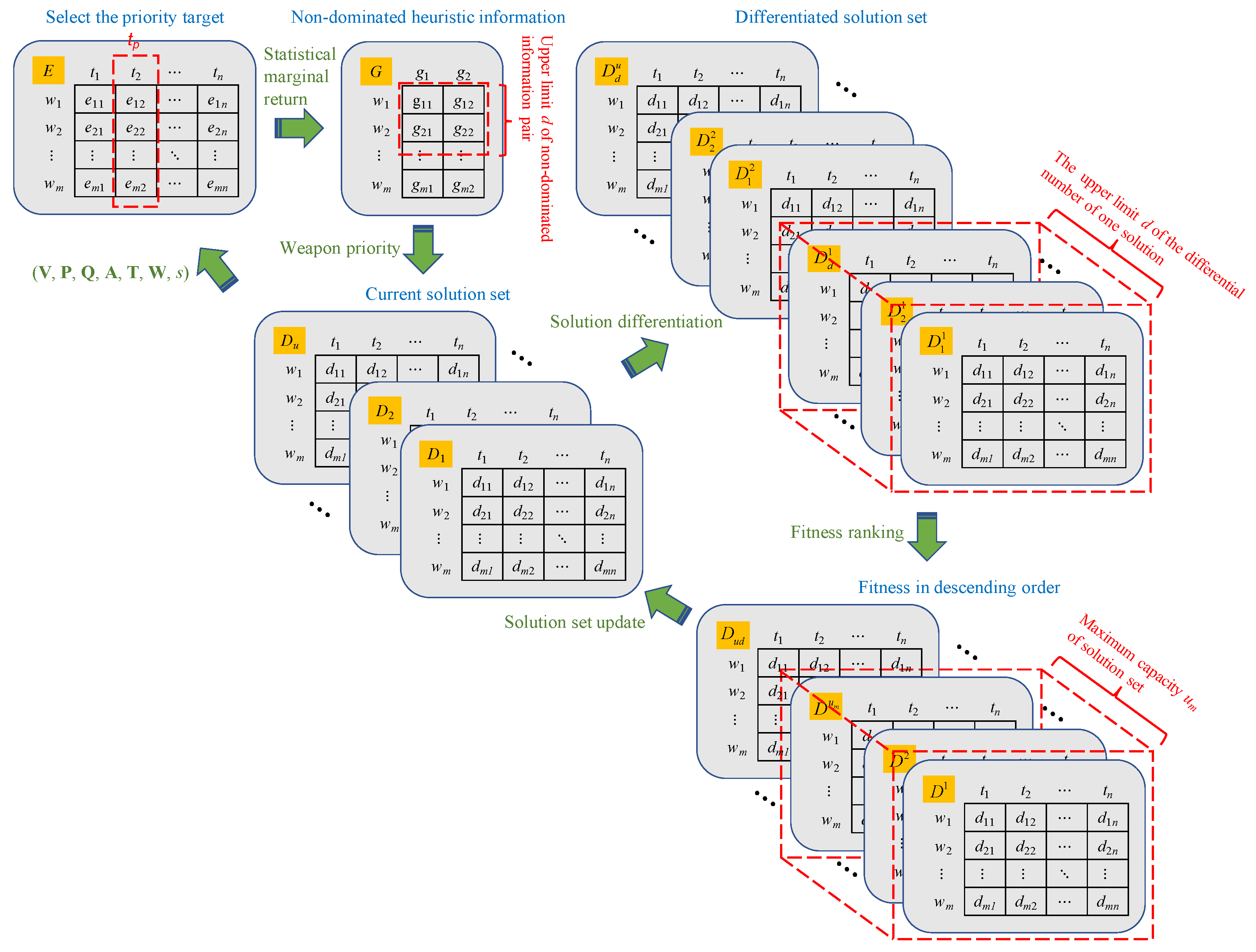
In summary, the A-DWTA decision method proposed in this paper is as follows: The current solution set of solution individuals is , where is the upper limit of the solution set, and r is the current weapon consumption. Extract a single solution , solve the priority defense asset and priority attack target , calculate the statistical marginal return information set of each weapon under “,” select the non-dominated information from G to form a new information set . Set the maximum number of differentiation for a single solution as d. If the number of non-dominated information pairs is greater than the differentiation number, that is, , d information pairs corresponding to d usable weapons are selected in descending order of , and is differentiated into K feasible solutions; otherwise, is directly differentiated into feasible solutions. Move the differentiated solutions to the differentiation set . Repeat the above process until all individuals in D complete the differentiation operation. Calculate each solution’s fitness in D, and select individuals with optimal fitness as the solution set for the next iteration. Repeat the above process until the algorithm termination condition is met. The flowchart of HA-SMR is shown in Figure 6.
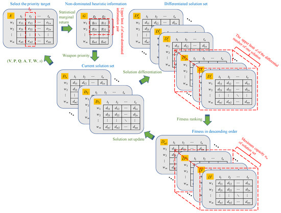
Figure 6.
Information flow of the weapon selection mechanism by the proposed heuristic information.
In HA-SMR, the designed differentiation strategy also reflects the diversity of the solution set, which can effectively avoid local optimal solutions. The reason for the generation of differentiated individuals in descending order is that considering the combat objectives of asset defense, the absolute return of killing targets at the current stage should take priority over the relative return.
4.3. Constraint Handling
In WTA problems, model constraints are usually used as algorithm termination conditions. In the model constraints (22), the constraint of marginal return expectation of a weapon is proposed. This constraint not only optimizes the decision efficiency-cost ratio but also controls the algorithm flow adaptively. As in step 7 of Algorithm 1, the weapon–target feasibility is updated as
where asset is the attack intention of target j as in Formula (31); is the weapon consumption threshold of Formula (20). Formula (35) shows that the assignment will reduce the cost–effectiveness ratio, and is allocated to other unmet threshold targets or retained for the next stage.
In the constraint conditions (22) of the A-DWTA model, the first three mathematical constraints have been satisfied by the coding method, and the fourth model constraint is also satisfied by the above termination condition. The dynamic constraints that need to be dealt with in the solving process are weapon–target feasibility constraints and target-resource feasibility constraints. According to the information flow of the algorithm, the observable variables connecting weapon, target, and resource are the weapon–target kill probability matrix , the weapon-target attack feasibility matrix , and the target–resource damage matrix . The algorithm employs the to update and , that is, set the component corresponding to the infeasible variable to 0, and there is no assignment return. For example, if indicates the following constraints: (1) weapon i is not available; (2) target j has been killed; (3) weapon i is available, and target j survives, but the attack condition of is not satisfied, namely . Similarly, if indicates: (1) target j has been killed; (2) asset k has been destroyed; (3) both target j and asset k are in a state of survival, but the attack intention of target j is not asset k. Through the above processing, the algorithm has been de-constrained, without additional constraint processing.
5. Experimental Studies
This section verifies the superiority of the A-DWTA/RH model and the HA-SMR proposed in this paper by setting experimental cases and comparison algorithms.
5.1. Operational Scenario and Performance Metrics
In the experiment section, the target–asset destroy intention, weapon–target attack condition is initialized and evolved by the following methods.
- (1)
- Target–asset destroy intention. Assuming that the defender is unknown to the targets’ attack strategy, and the threat assessment system identifies the target intention. The initialization method of target–asset destroy matrix is: (i) when targets are no fewer than assets (), the target intension is generated randomly on the premise that each asset is assigned at least one target. (ii) When there are more targets than assets (), the target intension is generated randomly under the premise that each target aims to different assets. The target–asset destroy probability is initialized aswhere and reflect the upper and lower bounds of target-asset vulnerability.
- (2)
- Weapon–target attack condition. The weapon-target kill probability is initialized bywhere and denotes the upper and lower bounds of weapon-target kill probability. In the evolution of subsequent stages, due to the operational state’s continuity, the weapon–target kill matrix of the current stage should be related to the weapon–target kill matrix, weapon state and target state of the previous stage. Let the transfer state of weapon–target kill probability follow
Weapon–target feasibility matrix of each stage refer to [37]
where means that the launch condition of i−j pair is met at stage s, otherwise ; is the probability threshold that weapon i can not launch for target j at stage s. The threshold decreases with the increase of the stage s, and the generated probability of zero elements in increases, which meet the evolution trend of attack uncertainty in the DWTA problem. and are the upper and lower bounds of the function , and is set a constant not less than the maximum stage number . is equal to 1 if its argument is positive and −1 otherwise.
From the application background of A-DWTA, the normalized asset value (NAV) is proposed as the dynamic metric. The weapon consumption and the number of stages are taken as the mission completion metric. Algorithm complexity and compute time are used as the real-time metric. The above metrics cover the operational requirements of decision-makers.
5.2. Experiments on Comparison Algorithms
The research on the A-DWTA problem is less than the research on the other WTA problems, and the models and solving algorithms proposed by each study are different, so it is not easy to make comparison under the same experimental framework. We select research with a similar model framework as the comparison group and adopt the verified algorithms as comparison algorithms: Hybrid Genetic Algorithm (HGA); Hybrid Ant-Colony Optimization (HACO); Memetic Algorithm based on Greedy Local Search (MA-GLS); Rule-based Heuristic Algorithm (RHA). Except, RHA has no parameter setting, the parameters of the model and comparison algorithms are as follows:
- A-DWTA/RH model: the weight of the absolute return expectation at the current stage = 0.6; the weight of the retun evaluation of remaining weapons on prediction situation = 1 − = 0.4;
- HA-SMR: The capacity of solution set = 50; the differentiation number d = 4; the threshold of weapon consumption = 0.85;
- HGA: the population size = 100; the number of elite individuals = 100; the crossover probability = 0.8; the mutation probability = 0.2;
- HACO: the population size = 200; the train importance factor = 1; the visibility importance factor = 2; the pheromone evaporation rate = 0.5;
- MA-GLS: the population size = 200; the crossover/mutation number of each generation is set to 10.
To complete the defense mission, the number of weapons should be no less than the number of targets. In order to compare the algorithms in different problem scales, the following method is used to generate experimental cases: randomly generate the number of targets n in different scale intervals ; randomly generate the number of weapons m in the interval ; and randomly generate the number of assets l in the interval , as shown in the formula. In the interval [1,100], the target number n is randomly generated with an interval of 10, and nine experimental cases generated are shown in Table 2.

Table 2.
The case scales of the algorithm comparison experiment.
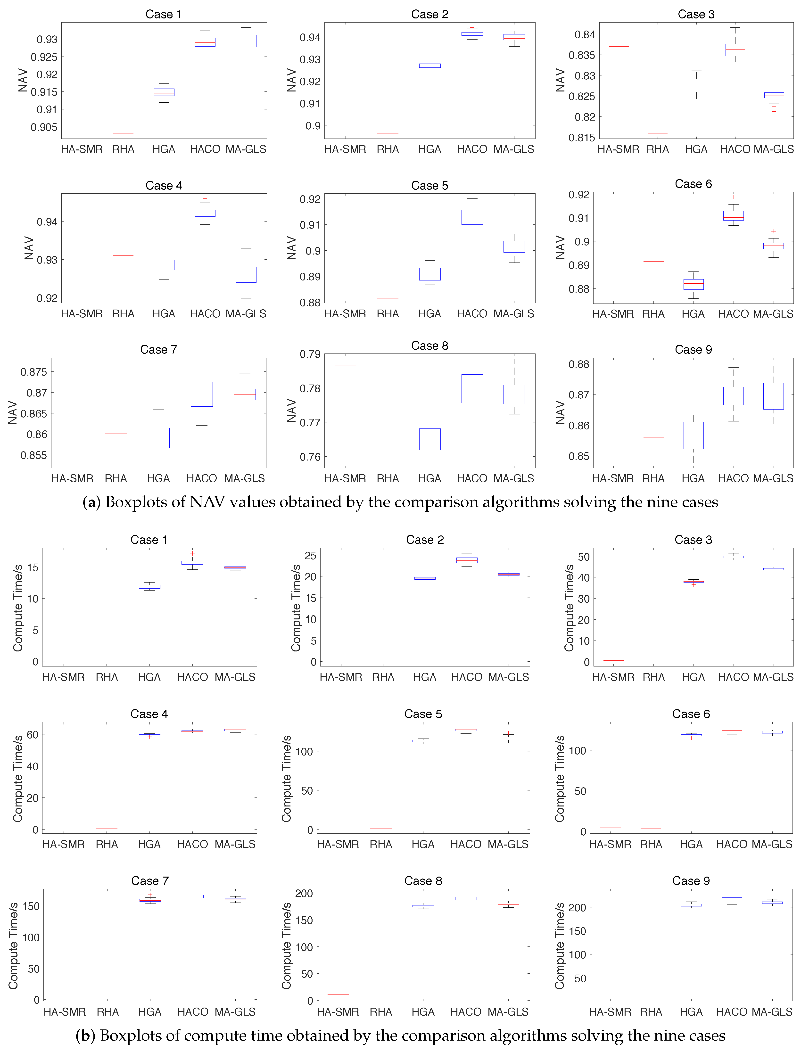
Let each comparison algorithm independently solve the above cases 30 times. The statistics of the experimental results are shown in Table 3, and the distribution of NAV and computational time is illustrated as box plots in Figure 7. A box plot is used to illustrate the distribution of metrics. The notches represent a robust estimate of the uncertainty about the medians for box-to-box comparison, and the symbol + denotes outliers.

Table 3.
Statistics of the results obtained by the comparison algorithms solving nine case over 30 independent runs.
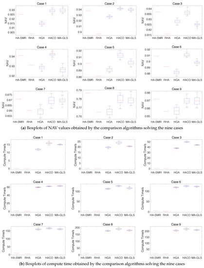
Figure 7.
Boxplots of normalized asset value (NAV) and compute time obtained by the comparison algorithms solving the nine instances over 30 independent runs.
Analyzing Table 3 and Figure 7, the mean value of NAV of HA-SMR is only 0.002∼0.005 lower than HGA and HACO in case 1 and 2, slightly lower than HACO in case 4–7, and better than other algorithms in case 8 and 9. The reason is that the SMR algorithm has no apparent advantages in convergence at a relatively small scale. However, owing to the problem scale and population size, the convergences of HGA, HACO, and MA-GLS are worse than HA-SMR. RHA can be considered as a particular case of HA-SMR in a single search direction, so the NAV of RHA is lower than HA-SMR. HA-SMR and RHA are deterministic algorithms, and the mean square error of NSVA is 0 theoretically. In the other swarming intelligent algorithms, the mean square errors of NAV are between 0.001 and 0.005 and increase with the increase of problem size. In terms of real-time performance, HA-SMR outperforms than the other algorithms, followed by RHA. The computational time of HA-SMR and RHA is in the same order of magnitude, while the other algorithms’ compute time is significantly higher than one order of magnitude. Similarly, the theoretical mean square error of two deterministic algorithms’ compute time is 0, and the mean square error of the other algorithms’ computational time increases with the problem scale, and is between 0 and 5 s. In conclusion, within the scale of W150T100A100, HA-SMR has better robustness in convergence, and balances the optimal and real-time effectively.
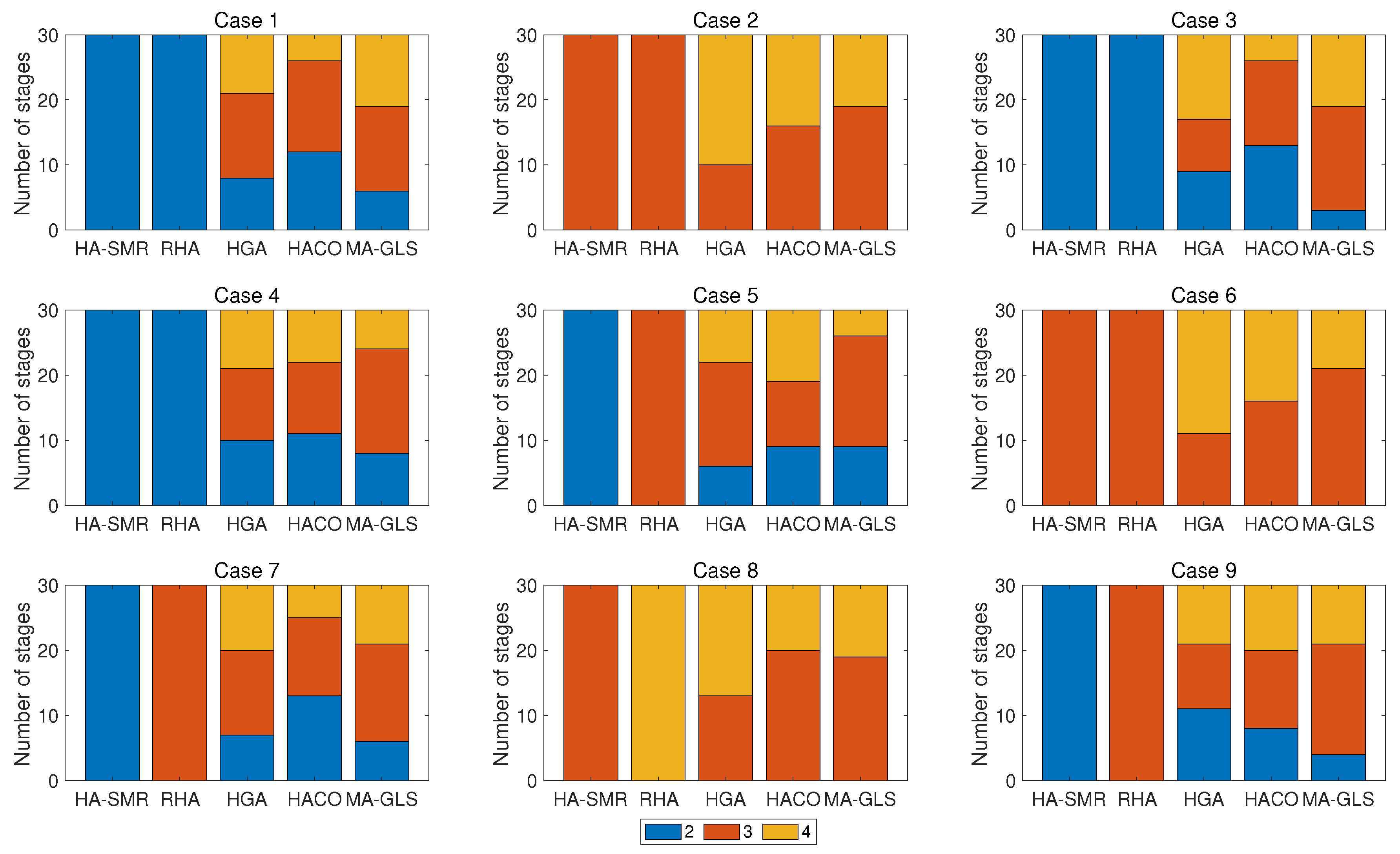
Besides NAV and computational time, minimizing the number of stages is also an essential operational requirement and a motivation of this paper. To verify the design of the SMR algorithm for “interception as soon as possible” combat requirements, Figure 8 shows the distribution of the actual number of stages obtained by each algorithm solving the same case 30 times independently.

Figure 8.
Distribution of the number of stages obtained by the comparison algorithms solving case 1∼9 of 30 runs independently.
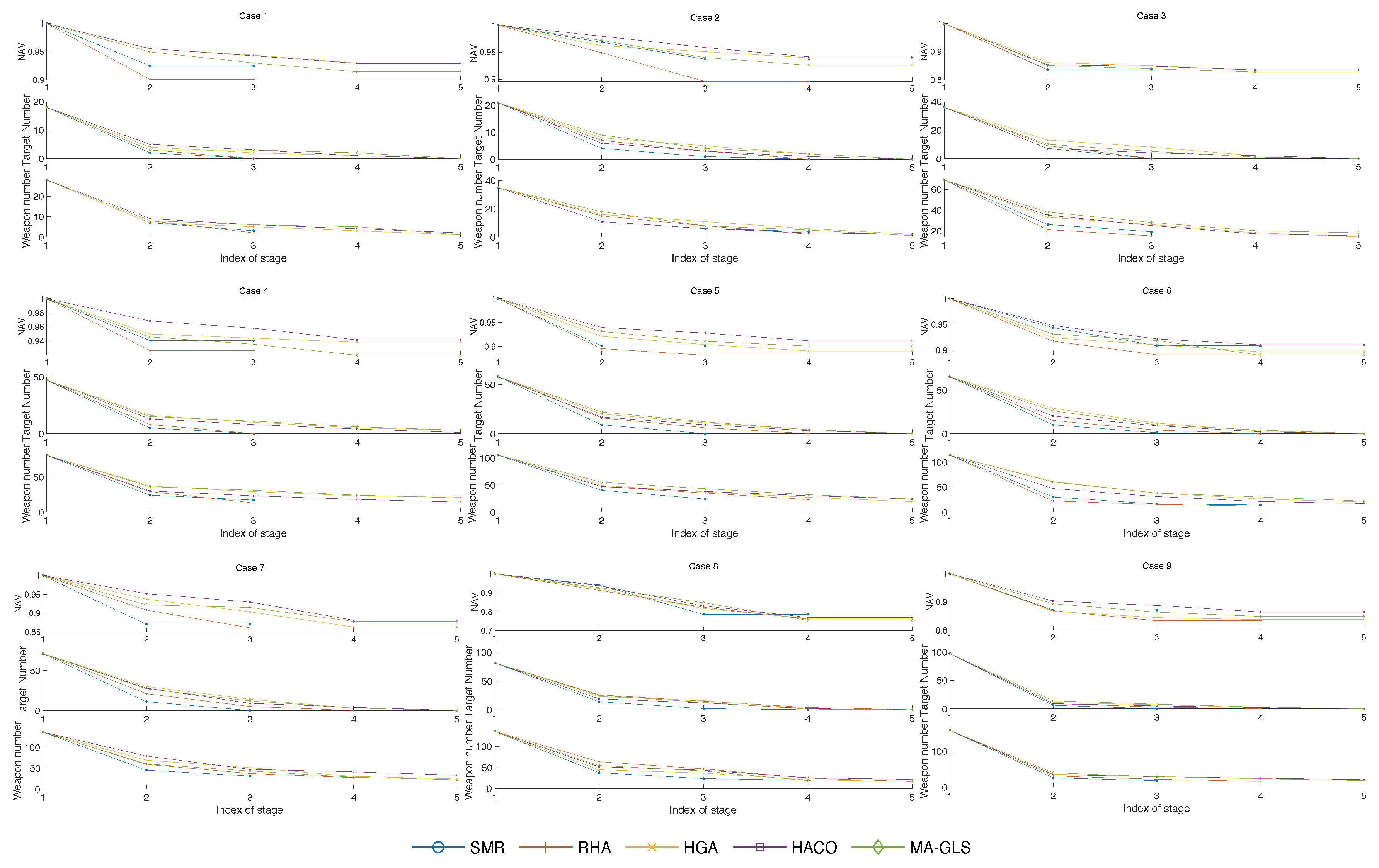
According to Figure 8, the number of stages of the decision plan obtained by HA-SMR solving the A-DWTA/RH model is less than other algorithms. When the problem scale is small (case 1 to 4), the number of stages obtained by HA-SMR and RHA is two or three. Let the number of decision stages of the HA-SMR algorithm be , then the number of stages obtained by HGA, HACO, and MA-GLS is distributed in the interval . The proportion of four stages solved by HACO is significantly less than that of HGA and MA-GLS. In conclusion, the scheme obtained by the HA-SMR algorithm can complete the target killing task in as few stages as possible. To further illustrate the advantages of HA-SMR through the weapon–target–asset states at each stage, Figure 9 shows the mean values of NMVA, remaining weapons, and surviving targets from the observe phase of each stage.
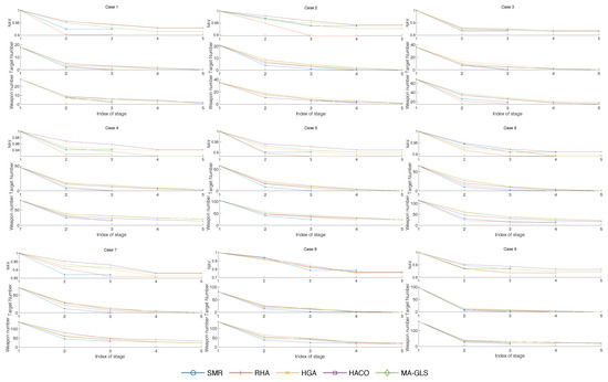
Figure 9.
Mean value of NAV, remaining weapons and surviving targets observed in each stage, obtained by the comparison algorithms solving case 1∼9 over 30 independent runs.
In Figure 9, HA-SMR and RHA consume more weapons at the 1st stage than the other algorithms, making the observed number of threat targets and remaining weapons drop rapidly at the 2nd stage. However, due to RHA’s greedy strategy, if the targets survive after the 1st stage, the remaining weapons in the 2nd or 3rd are less effective in killing the target. The statistical return strategy of HA-SMR maintains the remaining weapons still kill the surviving targets effectively. Due to the full-stage prediction mechanism, the other algorithms’ decision strategy is more conservative than HA-SMR, and the remaining weapons are less than HA-SMR when the operational mission is completed. It can be seen that the HA-SMR solving A-DWTA/RH has a better efficiency–cost ratio.
5.3. Parameter Sensitivity
In this section, the effects of specific parameters in the A-DWTA/RH model and HA-SMR on operational missions are analyzed experimentally.
5.3.1. Model Weight
In the A-DWTA/RH model, parameters are used to weigh the weapon consumption’s killing efficiency at the current stage against the counter-effectiveness of the remaining weapon. To analyze the influence on operational mission, is set up for simulation experiments. The problem scale of the example was W100T50A50, and the other variables are generated as the previous experiment. Under the different values of , the following three operational mission termination conditions are set:
- All assets are destroyed (), defense mission fails, let .
- Assets are not all damaged and targets are all killed ( and ), the defense task is completed, let .
- Assets have not been destroyed and targets have not been killed, but weapons have been consumed (, and ). It is predicted that the defense mission will fail, and let .
The experimental results of each case under the above parameter settings are shown in Table 4.

Table 4.
Experiment results of W100T50A50 under different values of .
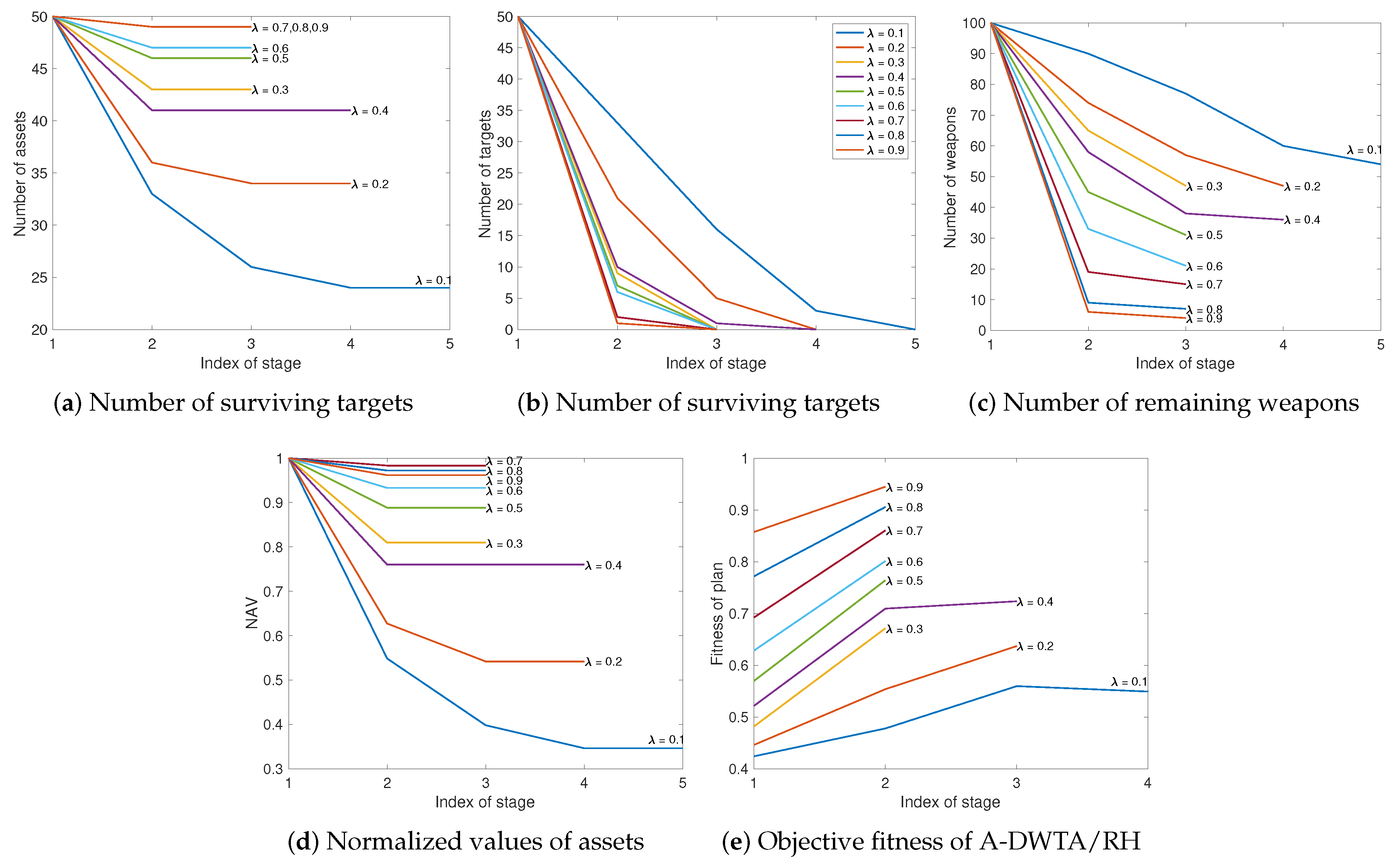
To further analyze the dynamic performance of HA-SMR solving the A-DWTA/RH under different value, Figure 10 gives the plot of the number of surviving assets, the number of surviving assets targets, the number of remaining weapons, NAV, and plan fitness observed at each stage.
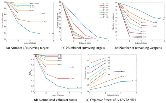
Figure 10.
The dynamic performance of the number of assets/targets/weapons, NAV and plan fitness under from 0.1 to 0.9.
In Table 4 and Figure 10, with the parameter increases from 0.1 to 0.9, the number of decision stages decreases from 4 to 2, and the compute time decreases from 3.3302s to 1.2706s. The reason is that A-DWTA/RH’s objective F is composed of the current decision’s kill effect and the remaining weapons’ counter effect after execution. represents the weight of the former. When is small, the decision plan will be guided to limit the weapon consumption of the current stage and retain the countermeasures in subsequent stages, which leads to an increased number of stages and computational time. The maximum value of NAV is 0.9832 at , and the fitness metric increases with the increase of . It can be seen that the objective F of A-DWTA/RH is more sensitive to than . Even when , there is no situation of excessive weapon consumption at the current stage and no counter weapons at the later stage (). In the mission termination sate, the defender can complete the mission () under the different value. However, as the value increases, the proportion of the current stage’s decision return increases, and the weapon consumption of the current stage also increase. So the number of surviving assets increases when the operational mission is completed. It is worth noting that when is 0.7, 0.8, and 0.9, the number of surplus weapons keeps decreasing, 15, 7 and 4 respectively. However, the number of decision stages and surviving targets remains unchanged, 2 and 49, respectively. It can be seen that if is higher than 0.7, weapon resource is easily wasted. In conclusion, the model parameter has the effect of balancing the “radical–conservative” degree of the decision plan, and the reasonable value is between 0.6 and 0.8.
5.3.2. Problem Scale
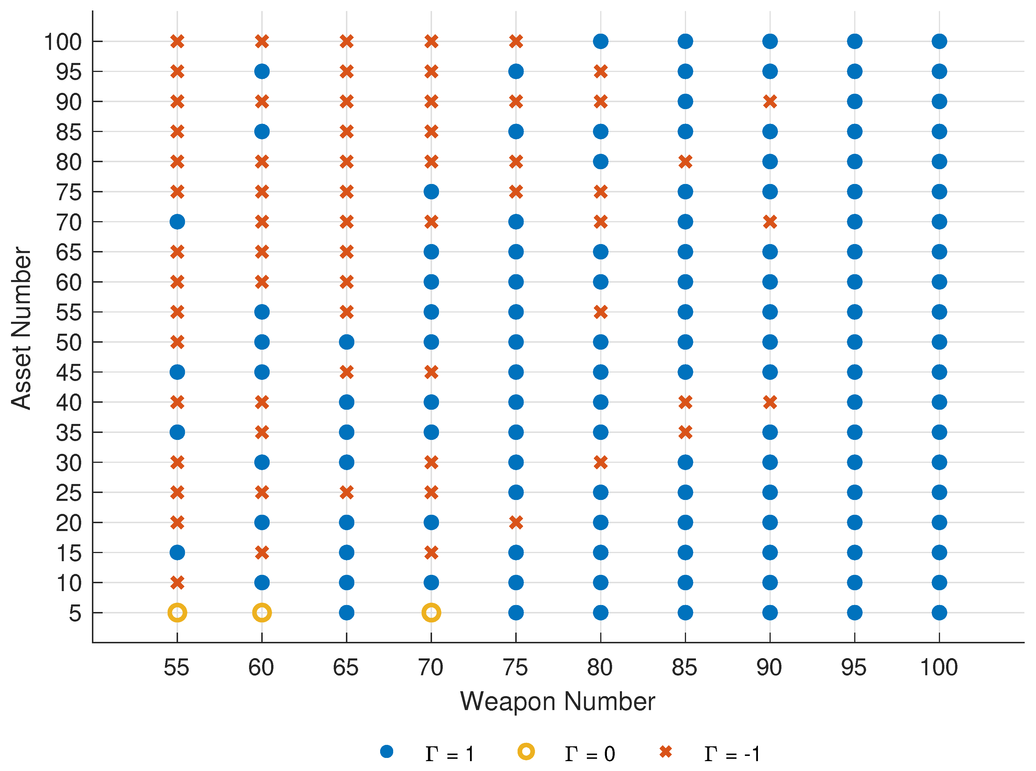
In case 9 of Table 4, the surplus number of weapons is only 4. Hence the relationship between the scale of weapon–target–asset directly affects the completion of the combat mission. In order to provide reference and basis for the configuration of completing the A-DWTA/RH mission, the dynamic relationship among the scale of weapon–target–asset is experimentally analyzed. In this experiment, the target number is fixed to 50. To ensure the possibility of completing the mission, the weapons should be more than targets. The weapon number is set to in turn, and the asset number is set to . The model parameter is set to 0.8. The remaining variables are consistent with the previous experiment. As the scales and parameters of each case in this simulation are different, they can only be analyzed based on the win–loss indicator’s statistical data. The distribution of defense mission completion indicator is shown in Figure 11.
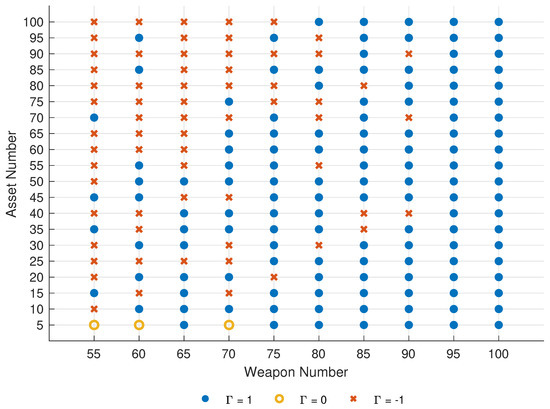
Figure 11.
The distribution of mission completion indicator under the scale of , , .
Illustrated by Figure 11, all assets are destroyed () only when the asset number is 5, and the weapon number is 55, 60, and 70. The reason is that the asset number is too small, and the weapon number is only 10% to 20% higher than the incoming target number, which cannot guarantee the survival probability of assets in a few stages. When the weapon number is less than 70, and the assets number rises to the target number (50), the situation of is basically obtained, that is, the weapons are fully used. The reason is that the weapon number is close to the target number, making it impossible to complete the defense mission. With the increase of asset number (), the target cannot destroy all assets in a few stages under the attack of weapons, so the weapons are consumed first. Finally, when the number of weapons is no less than 75, the probability of successful defense () increases significantly. When the number of weapons is no less than 95, the proportion of is 100%. In summary, regardless of the state of assets, the weapon number of 95% higher than the target number can ensure the completion of the defense mission.
5.3.3. Set Capacity and Differentiation Number D
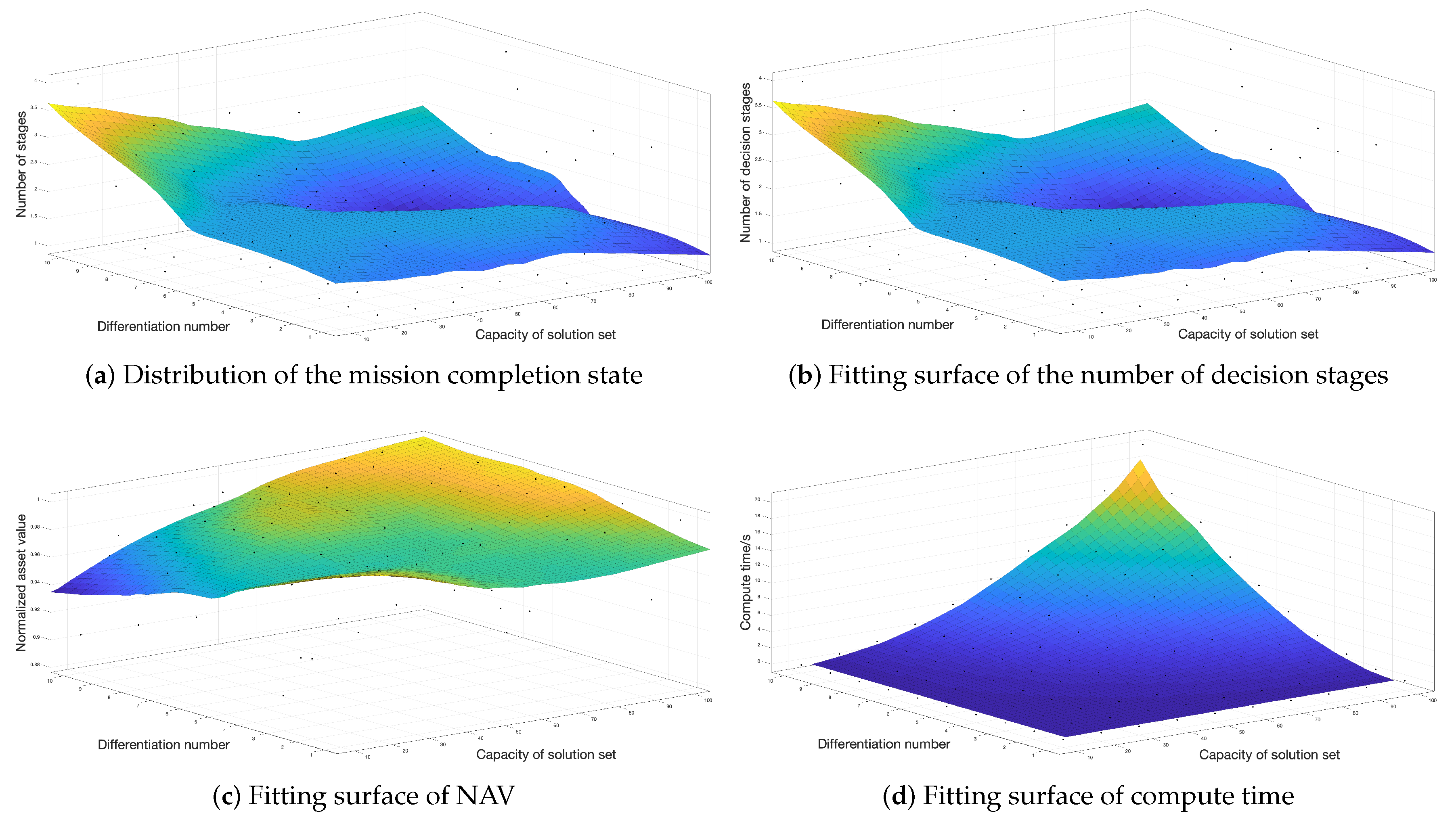
In HA-SMR, the solution set’s capacity and the differentiation number d of a single solution are the essential parameters to control the search space. The following cases are set to verify the influence of and d on HA-SMR: In the initial stage, weapon number m is set to 80; the target number n is set to 50; the asset number l is set to 50; the weapon-target kill probability and the target-asset damage matrix are generated by a formula, and the weapon consumption threshold is set to 0.8. Let the capacity of solution set be = [10:10:100], and the differentiation number be d = [1:1:10]. Figure 12 gives the fitting surface of four metrics distribution under different solution set capacity and differentiation number d.

Figure 12.
Fitting surface of four performance metric distribution of different set capacity and differentiation number d.
Figure 12a shows that the capacity and differentiation number d have no impact on the completion of the defense mission. The deterministic convergence mechanism of HA-SMR can give an effective solution under different values of and d. In Figure 12b, the number of decision stages decreases with the increase of the solution set’s capacity , and increases with the increase of the differentiation number d. According to Figure 12c, increasing the values of and d can improves NAV metric. In Figure 12d, when the value of rises from 10 to 100 and the value of d rises from 1 to 10, the compute time increases from 0.0064 s to 20.1675 s. In conclusion, on the premise of satisfying the real-time, the capacity of the solution set should be increased, and the number differentiation number d can be set to 5. Continue to increase the value of d do not significantly improve NAV, and burden the number of decision stages and compute time.
5.3.4. Threshold Parameter
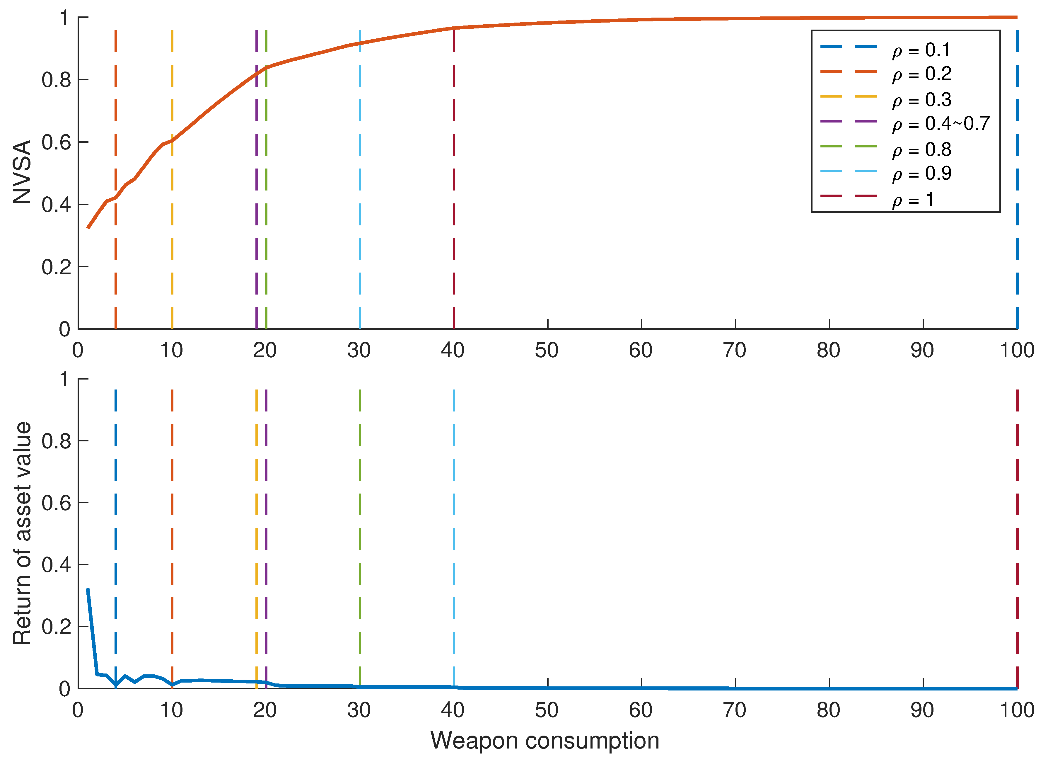
To verify the threshold of weapon consumption in HA-SMR, the following cases are set: in the initial stage, the weapon number m is set to 100; the target number is set to 20; the asset number is set to 20; the weapon-target kill probability and the target-asset destroy matrix are generated by a formula, and the solution set’s capacity and differentiation number d are set to 100 and 5. Let the threshold be = [0.1:0.1:0.1], and adopt HA-SMR to solve A-DWTA/RH model. Record the number of weapons consumed in the first stage under different values, and the plot of NAV and NAV return with the increase of weapon consumption, as shown in Figure 13.
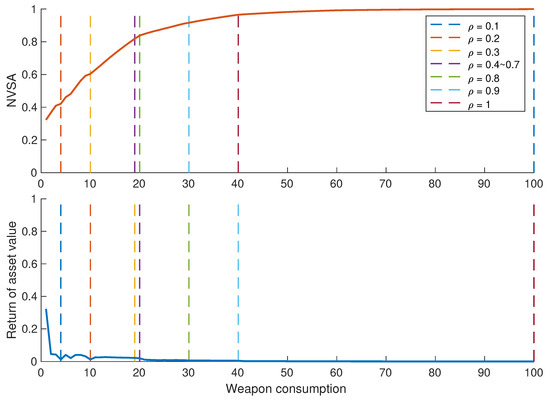
Figure 13.
Plots of weapon consumption, NAV and NAV return under different values of .
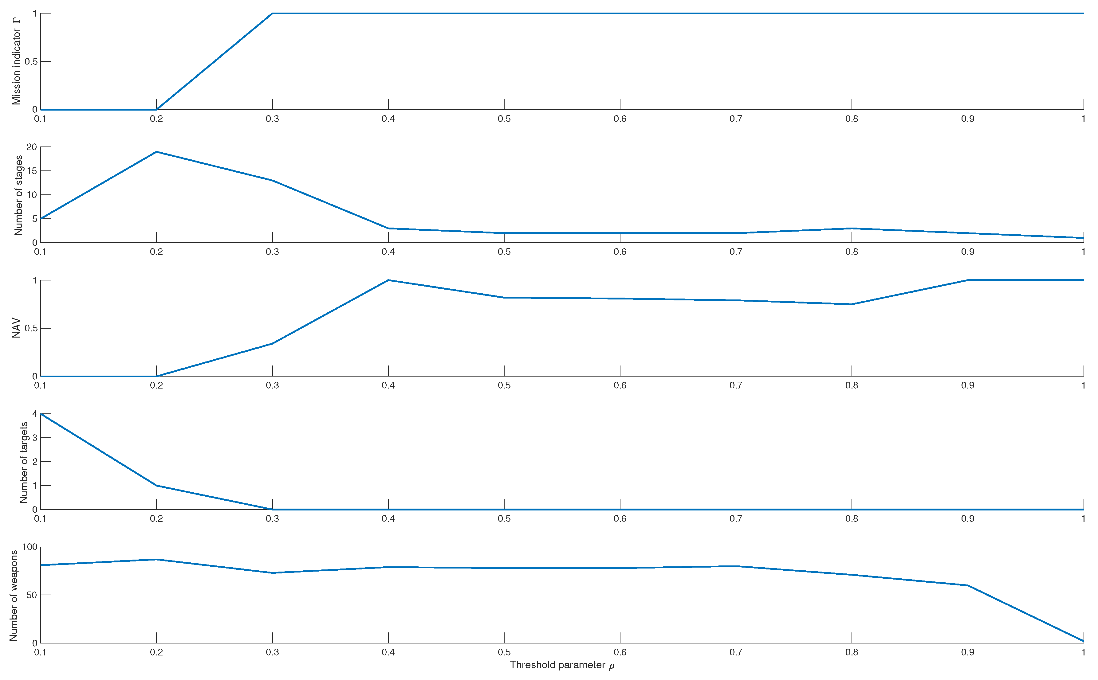
To further analyze HA-SMR dynamic performance under different values, Figure 14 shows the mission completion state, the number of decision stages, the normalized asset value, the number of surplus weapons, and the number of surviving targets when the threshold is 0.1 to 0.9. In Figure 14, the defense mission cannot be completed ( = 0) when the value of is 0.1 and 0.2. The assets are all destroyed by targets. The reason is that the value is too small to limit the weapon consumption at each stage, making the number of stages ( = 5, 19) and the number of surplus weapons large. When the value of rises from 0.3 to 0.9, the state of defense mission is ; the number of decision stages drops from 13 to 1; the number of surviving targets is 0, and the number of surplus weapons decreases from 73 to 2. The above metrics are relatively stable at of 0.3 to 0.7. Like the above experimental conclusion, of 0.7∼0.9 has better cost-effectiveness, which can minimize the number of decision stages, maximize the asset value and avoid waste of weapon resources on the premise of ensuring the completion of defense tasks.
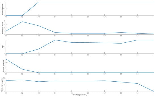
Figure 14.
The mission state, the number of decision stages, NAV, the number of surviving targets, and the number of surplus weapons under different values (0.1∼0.9).
6. Conclusions and Future Work
The major A-DWTA researches adopt the global return model based on multi-stage prediction, which can not fully reflect the operational requirement at the current stage and burden computing resource. From the above motivation, the A-DWTA problem is first analyzed by OODA theory. Then the A-DWTA/RH decision model is established, and the solving algorithm HA-SMR is designed. Experimental results show that the obtained decision plan can complete the defense mission in fewer decision stages than several comparison algorithms. The “radical–conservative” degree of the obtained plan can be adjusted by the model parameter and the algorithm parameter . The model weight is suggested as 0.6∼0.8, and the damage threshold is suggested as 0.7∼0.9.
The proposed heuristic information based on statistical marginal return is not only limited to the A-DWTA model, but also has a certain universality for weapon selection of various WTA problems. In this paper, the heuristic information is designed by the qualitative analysis of domain knowledge, and lacks rigorous theoretical verification. Aiming at the WTA of specific scenarios, design the corresponding weapon selection information by quantitative derivation, which is the future challenge.
Author Contributions
Conceptualization, K.Z.; methodology, K.Z. and Z.Y.; data curation, Y.Z.; Software, K.Z.; formal analysis, W.K. and Z.Y.; project administration, D.Z.; writing—original draft, K.Z.; writing—review and editing, Y.Z.; funding acquisition, D.Z. All authors have read and agreed to the published version of the manuscript.
Funding
This work was supported in part by the National Natural Science Foundation of China under Grant 61603299 and Grant 61612385, and in part by the Fundamental Research Funds for the Central Universities under Grant 3102019ZX016.
Acknowledgments
The authors greatly appreciate the reviews valuable suggestions and the editors encouragement.
Conflicts of Interest
The authors declare no conflict of interest.
References
- Roux, J.N.; Van Vuuren, J.H. Threat evaluation and weapon assignment decision support: A review of the state of the art. ORiON 2007, 23, 151–187. [Google Scholar] [CrossRef]
- Yang, Z.; Zhou, D.; Kong, W.; Piao, H.; Zhang, K.; Zhao, Y. Nondominated Maneuver Strategy Set with Tactical Requirements for a Fighter Against Missiles in a Dogfight. IEEE Access 2020, 8, 117298–117312. [Google Scholar] [CrossRef]
- Manne, A.S. A target-assignment problem. Oper. Res. 1958, 6, 346–351. [Google Scholar] [CrossRef]
- Hosein, P.A.; Athans, M. Preferential Defense Strategies. Part I: The Static Case; this Issue. 1990. Available online: https://core.ac.uk/download/pdf/4378993.pdf (accessed on 14 September 2020).
- Hosein, P.; Athans, M. Preferential Defense Strategies. Part 2: The Dynamic Case; LIDS-P-2003; MIT: Cambridge, MA, USA, 1990. [Google Scholar]
- Cai, H.; Liu, J.; Chen, Y.; Wang, H. Survey of the research on dynamic weapon-target assignment problem. J. Syst. Eng. Electron. 2006, 17, 559–565. [Google Scholar]
- Zhang, K.; Zhou, D.; Yang, Z.; Pan, Q.; Kong, W. Constrained Multi-Objective Weapon Target Assignment for Area Targets by Efficient Evolutionary Algorithm. IEEE Access 2019, 7, 176339–176360. [Google Scholar] [CrossRef]
- Murphey, R.A. Target-based weapon target assignment problems. In Nonlinear Assignment Problems; Springer: Berlin, Germany, 2000; pp. 39–53. [Google Scholar]
- Cho, D.H.; Choi, H.L. Greedy Maximization for Asset-Based Weapon-Target Assignment with Time-Dependent Rewards. Coop. Control Multi-Agent Syst. Theory Appl. 2017, 115–139. Available online: https://onlinelibrary.wiley.com/doi/10.1002/9781119266235.ch5 (accessed on 14 September 2020).
- Xin, B.; Wang, Y.; Chen, J. An efficient marginal-return-based constructive heuristic to solve the sensor– weapon–target assignment problem. IEEE Trans. Syst. Man Cybern. Syst. 2018, 49, 2536–2547. [Google Scholar] [CrossRef]
- Li, X.; Zhou, D.; Yang, Z.; Pan, Q.; Huang, J. A novel genetic algorithm for the synthetical Sensor-Weapon-Target assignment problem. Appl. Sci. 2019, 9, 3803. [Google Scholar] [CrossRef]
- Kline, A.; Ahner, D.; Hill, R. The weapon-target assignment problem. Comput. Oper. Res. 2019, 105, 226–236. [Google Scholar] [CrossRef]
- Hosein, P.A.; Athans, M. Some Analytical Results for the Dynamic Weapon-Target Allocation Problem; Technical Report; Massachusetts Inst of Tech Cambridge Lab for Information and Decision Systems: Cambridge, MA, USA, 1990. [Google Scholar]
- Eckler, A.R.; Burr, S.A. Mathematical Models of Target Coverage and Missile Allocation; Technical Report; Military Operations Research Society: Alexandria, VA, USA, 1972. [Google Scholar]
- Soland, R.M. Optimal terminal defense tactics when several sequential engagements are possible. Oper. Res. 1987, 35, 537–542. [Google Scholar] [CrossRef]
- Hosein, P.; Athans, M. The Dynamic Weapon-Target Assignment Problem; Technical Report; 1989; Available online: https://core.ac.uk/download/pdf/4380801.pdf (accessed on 14 September 2020).
- Leboucher, C.; Shin, H.S.; Siarry, P.; Chelouah, R.; Le Ménec, S.; Tsourdos, A. A two-step optimisation method for dynamic weapon target assignment problem. In Recent Advances on Meta-Heuristics and Their Application to Real Scenarios; InTech: Rijeka, Crotia, 2013; pp. 109–129. [Google Scholar]
- Zhengrong, J.; Faxing, L.; Hangyu, W. Multi-stage attack weapon target allocation method based on defense area analysis. J. Syst. Eng. Electron. 2020, 31, 539–550. [Google Scholar] [CrossRef]
- Jang, J.; Yoon, H.G.; Kim, J.C.; Kim, C.O. Adaptive Weapon-to-Target Assignment Model Based on the Real-Time Prediction of Hit Probability. IEEE Access 2019, 7, 72210–72220. [Google Scholar] [CrossRef]
- Lloyd, S.P.; Witsenhausen, H.S. Weapons allocation is NP-complete. In Proceedings of the 1986 Summer Computer Simulation Conference, Reno, NV, USA, 28–30 July 1986; pp. 1054–1058. [Google Scholar]
- Hocaoğlu, M.F. Weapon target assignment optimization for land based multi-air defense systems: A goal programming approach. Comput. Ind. Eng. 2019, 128, 681–689. [Google Scholar] [CrossRef]
- Cao, M.; Fang, W. Swarm Intelligence Algorithms for Weapon-Target Assignment in a Multilayer Defense Scenario: A Comparative Study. Symmetry 2020, 12, 824. [Google Scholar] [CrossRef]
- Kline, A.G.; Ahner, D.K.; Lunday, B.J. Real-time heuristic algorithms for the static weapon target assignment problem. J. Heuristics 2019, 25, 377–397. [Google Scholar] [CrossRef]
- Zhao, P.; Wang, J.; Kong, L. Decentralized Algorithms for Weapon-Target Assignment in Swarming Combat System. Math. Probl. Eng. 2019, 2019, 8425403. [Google Scholar] [CrossRef]
- Summers, D.S.; Robbins, M.J.; Lunday, B.J. An approximate dynamic programming approach for comparing firing policies in a networked air defense environment. Comput. Oper. Res. 2020, 117, 104890. [Google Scholar] [CrossRef]
- Fu, G.; Wang, C.; Zhang, D.; Zhao, J.; Wang, H. A Multiobjective Particle Swarm Optimization Algorithm Based on Multipopulation Coevolution for Weapon-Target Assignment. Math. Probl. Eng. 2019, 2019, 1424590. [Google Scholar] [CrossRef]
- Guo, D.; Liang, Z.; Jiang, P.; Dong, X.; Li, Q.; Ren, Z. Weapon-target assignment for multi-to-multi interception with grouping constraint. IEEE Access 2019, 7, 34838–34849. [Google Scholar] [CrossRef]
- Chen, J.; Xin, B.; Peng, Z.; Dou, L.; Zhang, J. Evolutionary decision-makings for the dynamic weapon-target assignment problem. Sci. China Ser. F Inf. Sci. 2009, 52, 2006. [Google Scholar] [CrossRef]
- Chang, T.; Kong, D.; Hao, N.; Xu, K.; Yang, G. Solving the dynamic weapon target assignment problem by an improved artificial bee colony algorithm with heuristic factor initialization. Appl. Soft Comput. 2018, 70, 845–863. [Google Scholar] [CrossRef]
- Wang, Y.; Li, J.; Huang, W.; Wen, T. Dynamic weapon target assignment based on intuitionistic fuzzy entropy of discrete particle swarm. China Commun. 2017, 14, 169–179. [Google Scholar] [CrossRef]
- Lai, C.M.; Wu, T.H. Simplified swarm optimization with initialization scheme for dynamic weapon–target assignment problem. Appl. Soft Comput. 2019, 82, 105542. [Google Scholar] [CrossRef]
- Shin, M.K.; Lee, D.; Choi, H.L. Weapon-Target Assignment Problem with Interference Constraints using Mixed-Integer Linear Programming. arXiv 2019, arXiv:1911.12567. [Google Scholar]
- Lee, D.; Shin, M.K.; Choi, H.L. Weapon Target Assignment Problem with Interference Constraints. In Proceedings of the AIAA Scitech 2020 Forum, Orlando, FL, USA, 6–10 January 2020; p. 0388. [Google Scholar]
- Xu, W.; Chen, C.; Ding, S.; Pardalos, P.M. A bi-objective dynamic collaborative task assignment under uncertainty using modified MOEA/D with heuristic initialization. Exp. Syst. Appl. 2020, 140, 112844. [Google Scholar] [CrossRef]
- Ahuja, R.K.; Kumar, A.; Jha, K.; Orlin, J.B. Exact and Heuristic Methods for the Weapon Target Assignment Problem; INFORMS: Catonsville, MD, USA, 2003. [Google Scholar]
- Lee, Z.J.; Su, S.F.; Lee, C.Y. Efficiently solving general weapon-target assignment problem by genetic algorithms with greedy eugenics. IEEE Trans. Syst. Man Cybern. Part B Cybern. 2003, 33, 113–121. [Google Scholar]
- Xin, B.; Chen, J.; Peng, Z.; Dou, L.; Zhang, J. An efficient rule-based constructive heuristic to solve dynamic weapon-target assignment problem. IEEE Trans. Syst. Man Cybern.-Part A Syst. Hum. 2010, 41, 598–606. [Google Scholar] [CrossRef]
- Leboucher, C.; Shin, H.; Le Ménec, S.; Tsourdos, A.; Kotenkoff, A. Optimal weapon target assignment based on an geometric approach. IFAC Proc. Vol. 2013, 46, 341–346. [Google Scholar] [CrossRef]
- Leboucher, C.; Shin, H.S.; Le Ménec, S.; Tsourdos, A.; Kotenkoff, A.; Siarry, P.; Chelouah, R. Novel evolutionary game based multi-objective optimisation for dynamic weapon target assignment. IFAC Proc. Vol. 2014, 47, 3936–3941. [Google Scholar] [CrossRef]
- Li, J.; Chen, J.; Xin, B.; Dou, L. Solving multi-objective multi-stage weapon target assignment problem via adaptive NSGA-II and adaptive MOEA/D: A comparison study. In Proceedings of the 2015 IEEE Congress on Evolutionary Computation (CEC), Sendai, Japan, 25–28 May 2015; pp. 3132–3139. [Google Scholar]
- Li, J.; Chen, J.; Xin, B.; Dou, L.; Peng, Z. Solving the uncertain multi-objective multi-stage weapon target assignment problem via MOEA/D-AWA. In Proceedings of the 2016 IEEE Congress on Evolutionary Computation (CEC), Vancouver, BC, Canada, 24–29 July 2016; pp. 4934–4941. [Google Scholar]
- Li, J.; Chen, J.; Xin, B.; Chen, L. Efficient multi-objective evolutionary algorithms for solving the multi-stage weapon target assignment problem: A comparison study. In Proceedings of the 2017 IEEE Congress on Evolutionary Computation (CEC), San Sebastian, Spain, 5–8 June 2017; pp. 435–442. [Google Scholar]
- Li, J.; Chen, J.; Xin, B. Optimizing multi-objective uncertain multi-stage weapon target assignment problems with the risk measure CVaR. In Proceedings of the 2019 IEEE 15th International Conference on Control and Automation (ICCA), Edinburgh, UK, 16–19 July 2019; pp. 61–66. [Google Scholar]
- Mei, Z.; Peng, Z.; Zhang, X. Optimal dynamic weapon-target assignment based on receding horizon control heuristic. In Proceedings of the 2017 13th IEEE International Conference on Control & Automation (ICCA), Ohrid, Macedonia, 3–6 July 2017; pp. 876–881. [Google Scholar]
- Kalyanam, K.; Casbeer, D.; Pachter, M. Monotone optimal threshold feedback policy for sequential weapon target assignment. J. Aerosp. Inf. Syst. 2017, 14, 68–72. [Google Scholar] [CrossRef]
- Duan, W.; Yuan, W.; Pan, L. Research on Algorithm for Dynamic Weapon Target Assignment Based on the Improved Markov Decision Model. In Proceedings of the 2018 37th Chinese Control Conference (CCC), Wuhan, China, 25–27 July 2018; pp. 8417–8424. [Google Scholar]
© 2020 by the authors. Licensee MDPI, Basel, Switzerland. This article is an open access article distributed under the terms and conditions of the Creative Commons Attribution (CC BY) license (http://creativecommons.org/licenses/by/4.0/).

