Renewable Energy Potential Estimation Using Climatic-Weather-Forecasting Machine Learning Algorithms

Abstract

The major challenge facing renewable energy systems in Nigeria is the lack of appropriate, affordable, and available meteorological stations that can accurately provide present and future trends in weather data and solar PV performance. It is crucial to find a solution to this because information on present and future solar PV performance is important to renewable energy investors so that they can assess the potential of renewable energy systems in various locations across the country. Although Nigerian weather provides favorable weather conditions for clean power generation, there is little penetration of renewable energy systems in the region, since over 95% of the power is fossil-fuel-generated. This is because there has been no detailed report showing the potential of clean power generation systems due to the dysfunctional meteorological stations in the country. This paper sought to fill this knowledge gap by providing a machine-learning-inspired forecasting of environmental weather parameters that can be used by manufacturing companies in evaluating the profitability of siting renewable energy systems in the region. Crucial weather parameters such as daily air temperature, relative humidity, atmospheric pressure, wind speed, and rainfall were obtained from NASA for a period of 19 years (viz. 2004–2022), resulting in the collection of 6664 high-resolution data points. These data were used to build diverse regressive neural networks with varying hyperparameters to find the best network arrangement. In summary, a low mean-squared error of 7 $\times$ 10⁻³ and high regression correlations of 96% were obtained during the training.

1. Introduction

Due to the increasing energy demand for economic development and the environmental issues associated with energy systems powered by fossil fuels, renewable energy systems have been globally accepted as an alternative source of energy [1]. In addition, in most developing nations such as Nigeria, there is a lack of a reliable and secure energy supply, and this has affected economic development [2]. Today, solar photovoltaics (PV) is one of the most notable and reliable renewable energy sources due to the availability of solar resources, the decrease in their energy cost, and their maximum energy production and efficiency [3]. Despite the benefits of solar PV, the technology is faced with complex and technical problems such as its dependency on climatic conditions; thus, favourable environmental conditions are necessary for optimal solar PV performance [4].

Unfortunately, meteorological stations that measure and predict environmental and geographical parameters for solar PV output are limited in Nigeria due to their cost of operation and the maintenance required for these stations [5,6]. Nigeria, being one of the most populated countries in the world with a population of almost 200 million and a land mass of 923,763 km², has only 54 weather observations stations, with some of the stations not functional and some not measuring all the environmental parameters needed for solar PV performance prediction [7]. Nigeria needs about 9000 weather stations to cover the data measurement across the country, and this is difficult to achieve at the moment; hence, it is necessary to find alternative means to measure and predict meteorological data across the country [8]. The accurate prediction of environmental conditions is important as it guarantees the safe operation and accurate estimation of solar PV performance, and hence allowing the economic integration of solar power systems into the grid.

Studies have investigated and developed different methods of estimating environmental conditions in Nigeria, such as statistical, mathematical, empirical and spatial interpolation models [9,10]. One of the recently developed methods is the application of artificial neural networks (ANNs), a subgroup of machine learning models, which was developed because of their accuracy and ability to model different and complex data [11] much more efficiently than conventional theoretical models [12]. Artificial neural networks (neural networks in short) are computational systems that are inspired by the biological thought process of the human brain, making them learn hidden trends in training data and making them able to accurately forecast data points outside of a given dataset [13]. Artificial neural networks have been applied in the past to forecast environmental weather parameters [12,14] and solar photovoltaic power output in different countries [15,16]; however, neural network models have been scarcely developed to accurately predict the environmental weather parameters of the Nigerian climate.

Bamisile et al. [17] developed an artificial neural network to predict the solar irradiance and PV power output operating in six locations in Nigeria. The artificial neural network was based on the general Levenberg–Marquardt algorithm, and the number of neurons varied from 200–2500, while the number of hidden layers varied from 1–4. The authors concluded that the developed model could accurately predict the solar irradiance and power output in Nigeria with a very high regression correlation of 0.98. The findings of this work were very commendable; however, the model only focused on predicting the solar irradiance levels in the states considered in the study. It has already been established that the output performance of a solar panel operating under outdoor conditions is dependent on other environmental factors such as the ambient temperature [18], wind speed [19], relative humidity [20], and even rainfall [21]. It was observed that the effects of these parameters on the power output and the performance of solar panels were not considered in the previous deep neural networks. The work assumed that solar irradiance was the major input parameter responsible for the PV’s performance; hence, little attention was paid to other crucial parameters in the forecasting of the developed neural network.

Ogunrinde et al. [22] predicted the monthly mean air temperature, solar irradiation, and precipitation obtained from five stations in Nigeria for a 12 month variation spanning 1985–2008. The training process was governed by the conventional Levenberg–Marquardt algorithm, and the transfer functions were based on the Tansig activation function. They reported that the optimum network had eight neurons in the hidden layer and that the root-mean-squared error during the testing period ranged from 0.28 to 0.82. The findings of these authors were very noteworthy; however, the resolution of the dataset they utilised during the training process was not large enough to give good insights regarding the hidden trends in the environmental weather parameters for the supposed data range. The paper reported that the training data was collected monthly over a monthly time step size for a period of 23 years (viz. 1985–2008). This implies that for each parameter, 12 $\times$ 23 = 276 datapoints were generated. These values were not enough to establish a precise artificial neural network, since the previous work in [17] on weather forecasting methods used an hourly time step spanning 12 years (2007–2018), which resulted in the generation of 105,120 data points for each parameter. It is also a general rule that larger datasets give higher neural network forecasting accuracies and are more reliable [23,24,25].

Ojo and Ogunjo [26] predicted monthly and annual rainfall amounts in Nigeria using two multivariate polynomial regressive models and twelve machine learning models including an artificial neural network model. The training data were obtained from 31 years of spatially distributed data recorded in Lagos, Nigeria, covering 16 climatic zones in Nigeria. The data were arranged in terms of monthly and annual time variations, and it was reported that the proposed models were very accurate in predicting the spatial rainfall distributions in Nigeria with a high-performance index of 0.906–0.996. The results provided by this study were quite commendable; nevertheless, only the rainfall amount was predicted by the proposed machine learning models. Other parameters that greatly affect the power output of solar photovoltaic systems were not considered in the model, making the model incapable of being applied to determining the solar photovoltaic performance in the studied locations in Nigeria. Similarly, Eichie et al. [27] developed a simple one-hidden-layer neural network based on the popular Levenberg–Marquardt algorithm to forecast the mean monthly air temperature recorded from ten weather stations covering different climatic zones for 34 year time span. The authors found that the optimum network comprised 37 neurons in the hidden layer, and the mean-squared error was 2.23, with the correlation coefficient ranging from 0.97 to 0.88. The results of the authors were very commendable; nevertheless, the resolution of the data was very small, spanning monthly air temperatures recorded every month for 34 years (34 $\times$ 12 = 408 datapoints only). This implies that the training data were not comprehensive enough to build the appropriate model needed to predict the air temperature.

Further research efforts have been made to predict environmental weather parameters for the Nigerian region using machine learning algorithms. Adams and Bamanga [28] proposed a seasonal rainfall forecasting model for Abuja, Nigeria, using a seasonal autoregressive integrated moving average method with data obtained from the Nigerian meteorological agency for the 1996–2018 time frame, and the analysis was conducted using the probability seasonal time series modelling method. The results indicated that the proposed model was able to forecast four years into the future, thus showing the efficacy of the model. Ighile et al. [29] predicted areas susceptible to flooding in Nigeria using artificial neural network and logistic regression models to build a flood susceptibility map. The artificial neural network (ANN) model had a 76.4% higher performance and a 62.5% higher flood prediction than the logistic regression model. In summary, the efficacy of the machine learning techniques in identifying regions prone to flooding was shown. AbdulRaheem et al. [30] compared three classical machine learning techniques—the decision tree (DT), k-nearest neighbourhood (KNN), and logistic regression (LR) models—in terms of their ability to model weather conditions for datasets obtained from the Kaggle website. The findings showed that the DT approach outperformed the KNN and LR models by 78% and 93%, respectively. Danbatta et al. [31] compared the performances of a proposed (ANN, polynomial, and Fourier series fitting) and a classical model (polynomial and Fourier series fitting models) in predicting the seasonal rainfall in northern Nigeria faced with insecurity challenges. The proposed models were also used to forecast the rainfall seasonality from 2022–2026 in selected regions of the nation. Edwin and Martins [32] forecasted the monthly rainfall seasonality of Ilorin, Nigeria, using four modelling schemes, i.e., the decomposition, square root transformation–deseasonalization, composite, and periodic autoregressive modelling schemes. It was concluded that the use of ANNs was more reliable, robust, and appropriate for rainfall seasonality prediction.

It is obvious that previous efforts have been made to build diverse artificial neural networks to predict the environmental weather parameters of the Nigerian climate due to the few and dysfunctional meteorological weather stations in the country. Nevertheless, it was observed that there have been very few efforts in the literature targeted at building accurate weather forecasting models based on artificial neural networks for the Nigerian climate. Furthermore, several previous efforts failed to consider all the environmental weather parameters that are needed to estimate the solar photovoltaic performance when cited in these locations, hence making the developed neural networks incomprehensive and incapable of being deployed in forecasting the solar potential in the Nigerian climate. Finally, it was noticed that some of the previous efforts relied on insufficient datasets with very low resolutions to develop the neural network models used in forecasting the environmental weather parameters for the Nigerian climate, hence casting doubts on the reliability of these models in accurately predicting the Nigerian weather conditions.

To fill the research gaps in the literature review, the current work sought to develop a comprehensive artificial neural network model to forecast the daily air temperature, relative humidity, pressure, wind speed, rainfall, and solar irradiance of Enugu, Nigeria for a period of 19 years (viz. 2004–2022), resulting in the collection of 6663 high-resolution data points. Furthermore, a hyper tuning of the network length was carried out by developing six neural network models comprising 10, 500, 1000, 1500, 2000, and 2500 neurons in a single hidden layer to select the network that best minimized the loss function while providing a good correlation between the targets and outputs, and at the same time, preventing overfitting. The current network should be able to fill the gaps present in the literature and accelerate the deployment of even more sophisticated neural networks such as deep neural networks in forecasting the solar photovoltaic potential in the Nigerian climate.

2. Methodology

2.1. Study Area

Enugu is situated in a tropical rainforest and descending savannah in the southeast geo-political zone of Nigeria with coordinates of 6.4483° N and 7.5139° E as shown in Figure 1. The yearly average rainfall in Enugu is about 2000 millimetres (79 in), which falls in sporadic amounts but intensifies throughout the rainy season. The only seasons that recur in Enugu are the rainy and dry seasons. The highest point of Enugu’s hills is 1000 metres (3300 ft). Generally speaking, sandstone underlies the highlands surrounding Enugu, while shale underlies the lowlands [33].

2.2. Data Gathering

The Modern-Era Retrospective analysis for Research and Applications (MERRA-2) version 2 web service [34] and Copernicus Atmosphere Monitoring Service (CAMS) radiation web service [35] were used to obtain the environmental weather data for a period of 19 years (viz. 2004–2022). The csv files obtained from the National Aeronautics and Space Administration (NASA) web services were imported to MATLAB R2020a using the csv read function, and the contents of the files were read and stored as variables in the workspace. The various parameters obtained were ambient temperature (2 m above ground level), relative humidity (2 m above ground level), pressure (at ground level), wind speed (10 m above ground level), rainfall (kg/m²), and beam and direct horizontal irradiation components (Wh/m²).

2.3. Data Analysis

Microsoft Excel was used to clean the data from the MERRA web service, while Python-PyCharm was used to sort the beam and diffuse horizontal irradiation data from CAMS to show the daily data distribution of the environmental parameters for the 19-year period. The global irradiation component was determined from the recorded beam, and the diffuse irradiation components were determined using the famous Lui–Jordan correlation [36]. The global irradiance was obtained by dividing the recorded global irradiation by 6, assuming 6 average hours of effective sunshine in the year range covered for Enugu, Nigeria [37].

2.4. Artificial Neural Network

In building a neural network for training our model, the MATLAB built-in nftool was used to train, test, and validate our network. To generate enough data points for the model training, 6664 data points derived from the number of days were used as the inputs. A MATLAB algorithm was developed to sort the data; thus, the data were normalized and unnormalized to develop a good model for training the outlier. The Levenberg–Marquardt backpropagation algorithm was utilized in this study to construct the network because of its great speed and effectiveness in learning. A total of 6 different networks with 10, 500, 1000, 1500, 2000, and 2500 neurons in a single hidden layer were constructed to achieve the optimum network architecture with a near-perfect regression plot, a very low mean-squared error, and a reduced overfitting tendency. The plots showed a comparison between the NASA dataset (target) and the ANN prediction (output).

The mean-squared error was used as the loss function in the present work. It was estimated using [38]

$$MSE=\frac{1}{n}{\sum }_{i=1}^n\left(Y_i-y_i\right)²$$

(1)

where n is the total number of observations/rows in the dataset, Y_i indicates the NASA input values, and $y_i$ indicates the neural-network-predicted values.

The regression correlation between the neural network predictions and the NASA input data was calculated using the Pearson correlation coefficient. This is a statistical parameter that determines how strong the relationship between 2 continuous variables is [39].

$$R=\frac{{\sum }_{i=1}^n\left(Y_i-{\tilde{Y}}_i\right)\left(y_i-{\tilde{y}}_i\right)}{\sqrt{{\sum }_{i=1}^n{\left(Y_i-{\tilde{Y}}_i\right)}^2{\sum }_{i=1}^n{\left(y_i-{\tilde{y}}_i\right)}^2}}$$

(2)

where ${\tilde{Y}}_i$ and ${\tilde{y}}_i$ are the mean values of the NASA data and neural-network-predicted values, respectively.

The list of parameters used for developing the neural network training process is listed in

Table 1. Network hyperparameters.

Network Type	Feed-Forward Back Propagation Network
Number of neurons	10, 500, 1000, 1500, 2000, and 2500
Performance	Mean-squared error (MSE)
Training algorithm	Levenberg–Marquardt algorithm

.

For training the process, measured samples for ten years (2004–2022) were used for training the ANN model, which totalled to 6664 data points; 70% of the dataset was used for training, 15% was used for testing, and 15% was used for validation.

2.5. Feature Normalization

During the data arrangement and cleaning, a normalization approach was used to convert the values of the dataset’s noise to a common scale of 0–1. When the ranges of the features in machine learning models are changed, it helped the mean-squared error (MSE) to look less noisy. The data should be normalized between values that are slightly off, such as 0.1 and 0.9. Scaling the input and output variables between (0.1, 0.9) is one method. Hence, according to ref. [40], feature normalization was carried out using the formula:

$$P_n=0.1+\frac{\left(0.9-0.1\right)\left(P-P_{min}\right)}{\left(P_{max}-P_{min}\right)}$$

(3)

where P_n is the normalized value of P, and P_max and P_min are the maximum and minimum values of P, respectively.

The simulation data needed to be un-normalized corresponding to the normalization after the neural network was trained, tested, and validated. This was achieved by making P the subject of the formula in Equation (3).

$$P=\frac{\left(P_n-0.1\right)\left(P_{max}-P_{min}\right)}{\left(0.9-0.1\right)+P_{min}}$$

(4)

where P is the unnormalized value of P_n.

2.6. Learning Algorithm for Artificial Neural Network

This section discusses the equations describing the back-propagation algorithm and the famous Levenberg–Marquardt algorithm used to build 1st-generation regressive neural networks.

2.6.1. Back Propagation Algorithm

Numerous studies have been conducted on artificial neural networks for classification and optimization issues [23,24,25]. Back propagation is used in multilayer neural networks as a training procedure. When applying the back propagation technique, the weights are altered in the network by moving in the negative direction of the gradient of the sum of the squared errors with regards to the weight variables. The error vector for a network with input, $x$, weights, $w$, targets, $t$, and outputs, $o$, is given as [41]:

$$\left[e\right]=\left[e\right]-\left[t\right]$$

(5)

The weights are then adjusted in a back propagation neural network as follows:

$$w_{t+1}=w_t-\eta \frac{1}{2}\frac{\partial e^{T}e}{\partial x}$$

(6)

where η is referred to as the learning parameter. Some related works have suggested using a momentum parameter µ [41]. When applying a momentum parameter, the weights will be updated with the following rule [41]:

$$w_{t+1}=w_t-\eta \frac{1}{2}\frac{\partial e^{T}e}{\partial x}+\mu \left(w_t-w_{t-1}\right)$$

(7)

2.6.2. Levenberg–Marquardt Algorithm

The Levenberg–Marquardt algorithm was adopted for use in our study; it is an alteration to the Gauss–Newton principle. The following rule was used to change the neural network training weights in the Gauss–Newton method [41]:

$$W_{n+1}=W\left(n\right)-{(J{\left(n\right)}^{T}J\left(n\right))}^{-1}J{\left(n\right)}^{T}e\left(n\right)$$

(8)

where$J$is the Jacobian matrix defined as [41]:

$$\mathrm{J}=\left[\frac{\partial e_1}{\partial w_1}\frac{\partial e_1}{\partial w_2} \dots \frac{\partial e_1}{\partial w_m}\frac{\partial e_2}{\partial w_1}\frac{\partial e_2}{\partial w_2}\dots \frac{\partial e_2}{\partial w_m} ⋮ ⋮ ⋮ \frac{\partial e_n}{\partial w_1}\frac{\partial e_n}{\partial w_2} \dots \frac{\partial e_n}{\partial w_m}\right]$$

(9)

The matrix inversion product result is dependent on the momentum parameter µ. This parameter will be determined by how the sum of squared errors is evaluated. The parameter is split by some scalar if the error is decreased.

3. Results and Discussions

This section portrays the results obtained from the different three-layer fully connected neural networks and shows the impact of hyperparameter tuning on the accuracy of the model at predicting future weather conditions. First, the precision of the feature-normalized ANN models is assessed in Section 3.1. Then, the results of the ANN training and the prediction of the daily environmental weather conditions in Enugu, Nigeria, using the different network parameters are presented in Section 3.2. Finally, Section 3.3 shows the effectiveness of selecting the right ANN model in predicting the weather conditions.

3.1. Error Analysis of the Feature-Normalized Models

The reliability of the different ANN results was determined by comparing the mean-squared error (MSE) and coefficient of correlation, R, plots of each model with the rest and selecting the model with the least error and the highest R values, respectively.

The precision of the ANN models needed to be evaluated before it could be deemed accurate to forecast the future weather conditions of Enugu, Nigeria. Figure 2 and Figure 3 show the validation results for the ANN models. The results shown in Figure 2 clearly show the changes in the mean-squared errors of the models with increment in the number of hidden units in our hidden layer.

The mean-squared-error plot helped to evaluate the nature of the fit provided by each ANN model. A training dataset is a dataset that is made of examples that are used during the learning process to fit the given parameters (inputs). The validation set provides a balanced assessment of a model’s fit on a given training dataset while modifying its hyperparameters, which include the number of hidden units (layer and layer widths) in an ANN. A test dataset is an independent dataset that follows the same probability distribution as the training dataset. It is used to evaluate the performance of the trained dataset. A minimal variation between the training and test errors represents a good effort in reducing overfitting in an ANN. The three cases of the fitting that an ANN model can provide are:

• Underfitting—high validation and training error;
• Overfitting—high validation error and low training error;
• Good fit—low validation error that is slightly higher than the training error [8].

This section discusses the equations describing the back-propagation algorithm and the famous Levenberg–Marquardt algorithm used to build first-generation regressive neural networks. Figure 2a,b show that the training, validation, and test errors of our ANN models with 10 (>10⁻² at two hundred and sixty-four epochs) and 500 (~10⁻² at five epochs) hidden units were all close together and were high (underfitting). Figure 2c displays that the validation and test error of our ANN model with 1000 hidden units was low (~10⁻² at four epochs) and slightly higher than its training error. Figure 2d–f show that the validation and test errors of our ANN models with 1500 (~10⁻² at four epochs), 2000 (>10⁻² at five epochs), and 2500 (>10⁻² at five epochs) hidden units were considerably higher than their training errors (overfitting).

Hence, Figure 2c indicates that the ANN model with 1000 hidden units in its hidden layer presented a good fit of the data since the validation error was low (~10⁻² at four epochs) and was slightly higher than the training error.

The coefficient of correlation, R, is a statistical measure of the strength of the relationship between a given dataset (input) and an ANN’s output data (target). Its value ranges from 0 to 1. A value of 0 represents no correlation, while a value of 1 indicates a perfect correlation.

Figure 3a shows the R value for the training, validation, and test sets for the ANN model with 10 hidden units, with an overall R value of 0.87298. Figure 3b–f display the train, validation, and test R values for the ANN models with 500, 1000, 1500, 2000, and 2500 hidden units with the best R values of 0.94349, 0.94957, 0.94933, 0.94236, and 0.93868, respectively.

Consequently, Figure 3c shows that for the model with 1000 hidden units, the validation, test, and even the best data, the value of R was the highest. The model with 2500 hidden units recorded the highest training data R value; however, the R values for the validation, test, and best data were significantly low. This confirmed that the model overfitted the dataset. From the plots, it was evident that the computation of the 1000-hidden-unit ANN model had the highest accuracy.

3.2. Predictions of Daily Weather Conditions by the ANN Models

The different forecasts of the daily weather condition made by the ANN models based on their level of accuracy are discussed in this section. The predicted weather conditions were plotted against the data collected from NASA’s Modern-Era Retrospective Analysis for Research and Applications (MERRA) online repository and compared.

3.2.1. Ambient Temperature

The ambient temperature plots of the collected NASA data versus the ANN predictions are shown in Figure 4. Moving from Figure 4a–f, it can be seen that the ANN plot became more like the NASA data as the number of hidden units in the hidden layer of the neural network increased.

3.2.2. Relative Humidity

Figure 5 shows the relative humidity plots of the collected NASA data against the ANN predictions. It can be seen that the accuracy of the ANN model’s predictions improved as the hidden neurons increased in number, as shown in Figure 5a–f.

3.2.3. Pressure

Figure 6a–f display the atmospheric pressure plots of the collected NASA data versus the ANN predictions. It can be seen that the precision of the ANN model’s predictions increased as the hyperparameters were tuned accordingly.

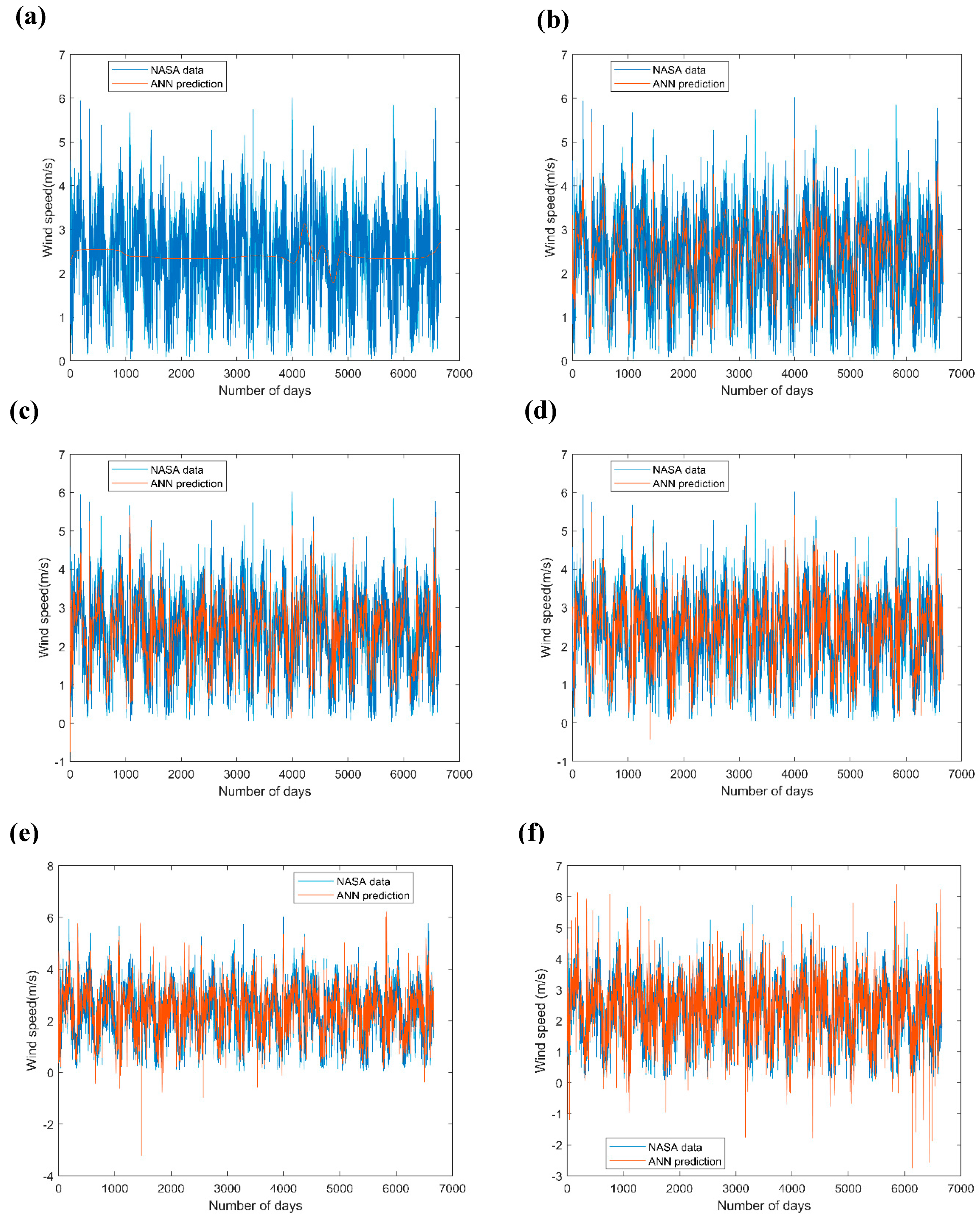
3.2.4. Wind Speed

The plots of the wind speed data collected from NASA is compared with the ANN model forecasts in Figure 7a–f. It can be seen that the accuracy of the ANN model’s predictions was affected by the number of hidden units in the neural network as it increased directly with the addition of more hidden units to the hidden layer.

3.2.5. Rainfall

The rainfall plots of the collected NASA data versus the ANN predictions are shown in Figure 8. Moving from Figure 8a–f, it can be seen that the ANN plot became more akin to the NASA data as the number of hidden units in the hidden layer of the neural network increased. However, Figure 8d–f indicates some irregularities in the ANN plot, where the predicted rainfall fell into the negative zone. This was because of the zero-mean step in our feature normalization process, where days with zero rainfall as represented in the NASA data were accounted for with negative integers in the normalized ANN model’s input matrix.

3.2.6. Solar Irradiance

Figure 9 shows the solar irradiance plots of the collected NASA data against the ANN predictions. It can be seen that the accuracy of the ANN model’s forecasts improved as the neurons in the hidden layer increase in number from Figure 9a–f. On careful observation, Figure 9f highlights an interesting concern about the upper limit in terms of the number of hidden units in the ANN hidden layer used in this study. Whereas in the other weather condition predictions the ANN model with 2500 hidden units gave a near-perfect plot compared to the NASA data, in this case, we can see that there was still a significant room for improvement in the accuracy of the ANN model.

3.3. Optimum ANN Model Selection

The intuition behind making the right choice for an ANN model is to examine the validation plots and compare them with the desired goal in mind. In this case, the aim was to create an ANN model that was as accurate as possible and could make good predictions for all the weather conditions examined in this study.

Looking at the mean-squared error and coefficient of correlation, R, plots in Figure 2 and Figure 3, the error and the R value decreased and increased, respectively, for the training dataset as the number of hidden neurons in the models became larger. For the validation and test sets however, the mean-squared error and the R value began to increase and decrease, respectively, after the 1000-hidden-neuron threshold. Hence, it is evident that the ANN model with 1000 hidden units in its hidden layer was the right choice. This model performed well on the training, validation, and test sets with a low error for all three groups that were not too far from each other. This indicated that the model could generalize well toward any other new data fed into it and could make accurate weather predictions.

The R plot for this model also recorded the highest value among all the ANN models considered in this paper. This showed that it recognized the highest relationship between the input data and the output it delivered.

The different forecasts of the daily weather condition made by the ANN models based on their level of accuracy are discussed in this section. The predicted weather conditions were plotted against the data collected from NASA’s Modern-Era Retrospective Analysis for Research and Applications (MERRA) online repository and compared.

4. Conclusions

Six neural network models were built in this paper to accurately forecast the weather parameters of Enugu, Nigeria, to facilitate the assessment of the solar potential of the region for possible photovoltaic power generation. The number of neurons in the single hidden layer varied between 10, 500, 1000, 1500, 2500, and 2500 to find how many neurons were optimal in accurately learning the trends in the high-resolution daily dataset collected from NASA spanning 19 years (2004–2022). The input parameter of the network was the number of days, and the predicted weather parameters were the air temperature, relative humidity, rainfall, pressure, and wind speed. Based on the analysis carried out, the following conclusions were made:

• The third neural network with 1000 neurons in the hidden layer was the best in fitting the given dataset while avoiding overfitting. This network terminated the training process after four epochs with a minimised mean squared error of 0.007 and high regression correlations of 0.96, 0.93, 0.92, and 0.95 for the training, cross-validation, testing, and all processes, respectively.
• Increasing the number of hidden neurons beyond 1000 for a single hidden layer resulted in an overlearning of the data, leading to inaccurate predictions outside the given dataset.
• The benchmark first neural network with 10 neurons in the hidden layer provided the worst fit of the data, with a mean squared error of 0.01 and low regression correlations of 0.87 for the training, cross-validation, testing, and all processes.
• Increasing the number of neurons was beneficial for the accuracy of the network depending on the data; however, beyond a specific number of neurons, the network began to overfit while consuming massive amounts of computational time with poor performances outside the input data.
• Several avenues for further research still arise from this work. For instance, the proposed models will be extended to forecast the weather parameters of the six geopolitical zones in the country and evaluate the total climatic weather distribution in the region. Thereafter, the forecasted weather parameters could be employed in directly estimating the performance of renewable energy devices, e.g., solar panels, operating in the country and provide reasonable estimations of the devices’ performances far into the future. These parameters could be used to evaluate the potential of solar PV systems operating in the climatic zones, informing renewable energy investors on the best places to invest in these renewable energy systems.
• It is recommended that a more sophisticated network such as a deep neural network with multiple hidden layers be used in the learning of the solar irradiance and rainfall parameters. This is because the selected third neural network was not able to fully capture the trends in these datasets. This will be the emphasis of a future study. Furthermore, the use of these parameters in evaluating the performance of a solar photovoltaic cell operating in the region will be conducted in the future study. Finally, the solar cell power and efficiency will be forecasted using the proposed deep neural network while divulging the best number of hidden layers and neurons to handle the massive data generated. This approach will also be extended to cover the six geopolitical zones of Nigeria, providing a suitable substitute to the unavailable and dysfunctional meteorological stations in the developing country with massive solar potential.

References

- Ab-Belkhair, A.; Rahebi, J.; Abdulhamed Mohamed Nureddin, A. A Study of Deep Neural Network Controller-Based Power Quality Improvement of Hybrid PV/Wind Systems by Using Smart Inverter. Int. J. Photoenergy 2020, 2020, 8891469. [Google Scholar] [CrossRef]
- Osinowo, A.A.; Okogbue, E.C.; Ogungbenro, S.B.; Fashanu, O. Analysis of Global Solar Irradiance over Climatic Zones in Nigeria for Solar Energy Applications. J. Sol. Energy 2015, 2015, 819307. [Google Scholar] [CrossRef]
- Verma, S.; Mohapatra, S.; Chowdhury, S.; Dwivedi, G. Cooling Techniques of the PV Module: A Review. Mater. Today Proc. 2020, 38, 253–258. [Google Scholar] [CrossRef]
- Zaraket, J.; Aillerie, M.; Salame, C. Capacitance Evolution of PV Solar Modules under Thermal Stress. Energy Procedia 2017, 119, 702–708. [Google Scholar] [CrossRef]
- Eludoyin, O.M.; Adelekan, I.O.; Webster, R.; Eludoyin, A.O. Air Temperature, Relative Humidity, Climate Regionalization and Thermal Comfort of Nigeria. Int. J. Climatol. 2014, 34, 2000–2018. [Google Scholar] [CrossRef]
- Shiru, M.S.; Shahid, S.; Dewan, A.; Chung, E.-S.; Alias, N.; Ahmed, K.; Hassan, Q.K. Projection of Meteorological Droughts in Nigeria during Growing Seasons under Climate Change Scenarios. Sci. Rep. 2020, 10, 10107. [Google Scholar] [CrossRef]
- Adaramola, M.S. Estimating Global Solar Radiation Using Common Meteorological Data in Akure, Nigeria. Renew. Energy 2012, 47, 38–44. [Google Scholar] [CrossRef]
- Ajayi, O.O.; Ohijeagbon, O.D.; Nwadialo, C.E.; Olasope, O. New Model to Estimate Daily Global Solar Radiation over Nigeria. Sustain. Energy Technol. Assess. 2014, 5, 28–36. [Google Scholar] [CrossRef]
- Abdel-Nasser, M.; Mahmoud, K. Accurate Photovoltaic Power Forecasting Models Using Deep LSTM-RNN. Neural Comput. Appl. 2019, 31, 2727–2740. [Google Scholar] [CrossRef]
- Antonopoulos, V.Z.; Papamichail, D.M.; Aschonitis, V.G.; Antonopoulos, A.V. Solar Radiation Estimation Methods Using ANN and Empirical Models. Comput. Electron. Agric. 2019, 160, 160–167. [Google Scholar] [CrossRef]
- Afram, A.; Janabi-Sharifi, F.; Fung, A.S.; Raahemifar, K. Artificial Neural Network (ANN) Based Model Predictive Control (MPC) and Optimization of HVAC Systems: A State of the Art Review and Case Study of a Residential HVAC System. Energy Build. 2017, 141, 96–113. [Google Scholar] [CrossRef]
- Ozoegwu, C.G. The Solar Energy Assessment Methods for Nigeria: The Current Status, the Future Directions and a Neural Time Series Method. Renew. Sustain. Energy Rev. 2020, 92, 146–159. [Google Scholar] [CrossRef]
- Maduabuchi, C. Thermo-Mechanical Optimization of Thermoelectric Generators Using Deep Learning Artificial Intelligence Algorithms Fed with Verified Finite Element Simulation Data. Appl. Energy 2022, 315, 118943. [Google Scholar] [CrossRef]
- Ghimire, S.; Deo, R.C.; Downs, N.J.; Raj, N. Global Solar Radiation Prediction by ANN Integrated with European Centre for Medium Range Weather Forecast Fields in Solar Rich Cities of Queensland Australia. J. Clean. Prod. 2019, 216, 288–310. [Google Scholar] [CrossRef]
- Garud, K.S.; Jayaraj, S.; Lee, M.Y. A Review on Modeling of Solar Photovoltaic Systems Using Artificial Neural Networks, Fuzzy Logic, Genetic Algorithm and Hybrid Models. Int. J. Energy Res. 2021, 45, 6–35. [Google Scholar] [CrossRef]
- Lo Brano, V.; Ciulla, G.; Di Falco, M. Artificial Neural Networks to Predict the Power Output of a PV Panel. Int. J. Photoenergy 2014, 2014, 193083. [Google Scholar] [CrossRef]
- Bamisile, O.; Oluwasanmi, A.; Obiora, S.; Osei-Mensah, E.; Asoronye, G.; Huang, Q. Application of Deep Learning for Solar Irradiance and Solar Photovoltaic Multi-Parameter Forecast. Energy Sources Part A Recovery Util. Environ. Eff. 2020, 1–21. [Google Scholar] [CrossRef]
- Ali, K.; Jia, Y.; Abbas, M.; Bukhari, S.A. Environmental Effects on the Performance of Polycrystalline Silicon Solar Cells under Long-Term Outdoor Exposure in Taiyuan, China. J. Power Energy Eng. 2019, 7, 15–27. [Google Scholar] [CrossRef]
- Bhattacharya, T.; Chakraborty, A.K.; Pal, K. Effects of Ambient Temperature and Wind Speed on Performance of Monocrystalline Solar Photovoltaic Module in Tripura, India. J. Sol. Energy 2014, 2014, 817078. [Google Scholar] [CrossRef]
- Dajuma, A.; Yahaya, S.; Touré, S.; Diedhiou, A.; Adamou, R.; Konaré, A.; Sido, M.; Golba, M. Sensitivity of Solar Photovoltaic Panel Efficiency to Weather and Dust over West Africa: Comparative Experimental Study between Niamey (Niger) and Abidjan (Côte d’Ivoire). Comput. Water Energy Environ. Eng. 2016, 5, 123–147. [Google Scholar] [CrossRef] [Green Version]
- Simsek, E.; Williams, M.J.; Pilon, L. Effect of Dew and Rain on Photovoltaic Solar Cell Performances. Sol. Energy Mater. Sol. Cells 2021, 222, 110908. [Google Scholar] [CrossRef]
- Ogunrinde, A.T.; Oguntunde, P.G.; Fasinmirin, J.T.; Akinwumiju, A.S. Application of Artificial Neural Network for Forecasting Standardized Precipitation and Evapotranspiration Index: A Case Study of Nigeria. Eng. Rep. 2020, 2, e12194. [Google Scholar] [CrossRef]
- Abdolrasol, M.G.M.; Suhail Hussain, S.M.; Ustun, T.S.; Sarker, M.R.; Hannan, M.A.; Mohamed, R.; Ali, J.A.; Mekhilef, S.; Milad, A. Artificial Neural Networks Based Optimization Techniques: A Review. Electronics 2021, 10, 2689. [Google Scholar] [CrossRef]
- Sarker, I.H. Deep Learning: A Comprehensive Overview on Techniques, Taxonomy, Applications and Research Directions. SN Comput. Sci. 2021, 2, 420. [Google Scholar] [CrossRef]
- Alzubaidi, L.; Zhang, J.; Humaidi, A.J.; Al-Dujaili, A.; Duan, Y.; Al-Shamma, O.; Santamaría, J.; Fadhel, M.A.; Al-Amidie, M.; Farhan, L. Review of Deep Learning: Concepts, CNN Architectures, Challenges, Applications, Future Directions. J. Big Data 2021, 8, 53. [Google Scholar] [CrossRef]
- Ojo, O.S.; Ogunjo, S.T. Machine Learning Models for Prediction of Rainfall over Nigeria. Sci. Afr. 2022, 16, e01246. [Google Scholar] [CrossRef]
- Ofure Eichie, J.; Oluwamayowa Agidi, E.; David Oyedum, O. Atmospheric Temperature Prediction across Nigeria Using Artificial Neural Network. In Proceedings of the ICFNDS 2021: The 5th International Conference on Future Networks & Distributed Systems, Dubai, United Arab Emirates, 15–16 December 2021; pp. 280–286. [Google Scholar] [CrossRef]
- Adams, S.; Bamanga, M. Modelling and Forecasting Seasonal Behavior of Rainfall in Abuja, Nigeria; A SARIMA Approach. Am. J. Math. Stat. 2020, 10, 10–19. [Google Scholar] [CrossRef]
- Ighile, E.H.; Shirakawa, H.; Tanikawa, H. Application of GIS and Machine Learning to Predict Flood Areas in Nigeria. Sustainability 2022, 14, 5039. [Google Scholar] [CrossRef]
- AbdulRaheem, M.; Awotunde, J.B.; Adeniyi, A.E.; Oladipo, I.D.; Adekola, S.O. Weather Prediction Performance Evaluation on Selected Machine Learning Algorithms. IAES Int. J. Artif. Intell. 2022, 11, 1535. [Google Scholar] [CrossRef]
- Danbatta, S.J.; Varol, A.; Nasab, A. Time Series Modeling and Forecasting of Expected Monthly Rainfall in Some Regions of Northern Nigeria Amid Security Challenges. In Proceedings of the 2022 3rd International Informatics and Software Engineering Conference (IISEC), Ankara, Turkey, 15–16 December 2022; pp. 1–6. [Google Scholar]
- Edwin, A.I.; Martins, O.Y. Stochastic Characteristics and Modelling of Monthly Rainfall Time Series of Ilorin, Nigeria. Open J. Mod. Hydrol. 2014, 4, 67–79. [Google Scholar] [CrossRef]
- Enete, I.; Alabi, M. Characteristics of Urban Heat Island in Enugu During Rainy Season. Ethiop. J. Environ. Stud. Manag. 2012, 5, 9–18. [Google Scholar] [CrossRef]
- Randles, C.A.; da Silva, A.M.; Buchard, V.; Colarco, P.R.; Darmenov, A.; Govindaraju, R.; Smirnov, A.; Holben, B.; Ferrare, R.; Hair, J.; et al. The MERRA-2 Aerosol Reanalysis, 1980 Onward. Part I: System Description and Data Assimilation Evaluation. J. Clim. 2017, 30, 6823–6850. [Google Scholar] [CrossRef] [PubMed]
- Schroedter-Homscheidt, M.; Arola, A.; Killius, N.; Lefèvre, M.; Saboret, L.; Wandji, W.; Wald, L.; Wey, E. The Copernicus Atmosphere Monitoring Service (CAMS) Radiation Service in a Nutshell. In Proceedings of the 22nd SolarPACES Conference 2016, Abu Dhabi, United Arab Emirates, 11–14 October 2016; pp. 1–4. [Google Scholar]
- Mbah, O.M.; Mgbemene, C.A.; Enibe, S.O.; Ozor, P.A.; Mbohwa, C. Comparison of Experimental Data and Isotropic Sky Models for Global Solar Radiation Estimation in Eastern Nigeria. In Proceedings of the World Congress on Engineering 2018, London, UK, 4–6 July 2018; Volume II, pp. 4–8. [Google Scholar]
- Does Solar Energy Work Everywhere in Nigeria? Available online: https://solyntaenergy.com/2018/01/04/does-solar-work-everywhere-in-nigeria/#:~:text=There%20is%20an%20average%20of,74.6°%20above%20the%20horizon (accessed on 5 December 2022).
- Pang, Z.; Niu, F.; O’Neill, Z. Solar Radiation Prediction Using Recurrent Neural Network and Artificial Neural Network: A Case Study with Comparisons. Renew. Energy 2020, 156, 279–289. [Google Scholar] [CrossRef]
- Schober, P.; Boer, C.; Schwarte, L.A. Correlation Coefficients. Anesth. Analg. 2018, 126, 1763–1768. [Google Scholar] [CrossRef]
- Gangi Setti, S.; Rao, R.N. Artificial Neural Network Approach for Prediction of Stress–Strain Curve of near β Titanium Alloy. Rare Met. 2014, 33, 249–257. [Google Scholar] [CrossRef]
- Reynaldi, A.; Lukas, S.; Margaretha, H. Backpropagation and Levenberg-Marquardt Algorithm for Training Finite Element Neural Network. In Proceedings of the 2012 Sixth UKSim/AMSS European Symposium on Computer Modeling and Simulation, IEEE, Washington, DC, USA, 14–16 November 2012; pp. 89–94. [Google Scholar]