On the Wigner-Kirkwood Expansion of the Free Energy and the Evaluation of the Quantum Correction

Abstract

The Wigner-Kirkwood expansion of the quantum correction to the classical free energy is generally said to be in powers of ${\hslash }^2$ and only its first few terms are presented. In this work, we use the Bloch differential equation to obtain a general description of all terms in a dimensionless form. The first corrective term turns out to be proportional to the product of ${\lambda }^2/a^2$, where $\lambda$ is the thermal de Broglie wavelength and $a^3$ is the volume per particle, by an effective coupling constant. This dimensionless parameter can be used to assess the magnitude of the quantum correction. Using the one-component plasma as an illustration we highlight the importance of the magnitude of the potential on the quantum correction. The results presented are not formally new; the emphasis is placed on a simple and didactic presentation.

1. Introduction

Describing the physical properties of matter under a wide range of thermodynamic conditions requires a very diverse set of tools. At low density one can easily use classical approximations, even though ionization effects have to be properly included as temperature increases. But as the density increases one needs to include N-body interactions as well as quantum effects. For low temperatures degeneracy effects become also important. The most complicated systems are probably the ones involving condensed and warm dense matter for which electrons are degenerate and even the nuclei can have a quantum behavior.

Quantum Monte-Carlo (QMC) simulations [1] or path-integral molecular dynamics (PIMD) [2] are able to tackle such systems but with a very high computer cost. At higher temperatures one can advantageously consider nuclei as classical and use Kohn-Sham-density-functional-theory-based molecular dynamics (see references in [3]), path-integral Monte-Carlo [4,5] or even pseudo-atom molecular dynamics [6]. But these techniques are still very computer-time-consuming and it is important to determine what is the proper physics to include and to determine the extent of N-body and quantum effects so as to choose the appropriate tool. The N-body effects can be advantageously anticipated by the consideration of coupling parameters. For the quantum behaviors it is a bit more difficult to properly anticipate their importance.

The thermodynamic properties of a system can be obtained from the partition function Q defined in the canonical ensemble by [7]

$$Q=\mathrm{Tr}(e^{-\beta \widehat{H}}),$$

(1)

where $\widehat{H}$ is the Hamiltonian operator of the system, $\mathrm{Tr}$ denotes the trace of the argument, and $\beta =1/\left(k_{\mathrm{B}}T\right)$, where T is the temperature of the system and $k_{\mathrm{B}}$ is Boltzmann’s constant. In the classical limit of Boltzmann statistics, the partition function can be simplified and taken equal to [7]

$$Q_{\mathrm{cl}}=\frac{1}{h^{3N}N!}\int \int exp(-\beta H)\mathrm{d}\mathbf{r}\mathrm{d}\mathbf{p},$$

(2)

where h is Planck’s constant, N is the number of atoms of the system, m is the mass of the atoms (they are assumed to be identical for the sake of simplicity), $H={\mathbf{p}}^2/2m+V\left(\mathbf{r}\right)$, $\mathbf{r}=({\mathbf{r}}_{\mathbf{1}},\cdots ,{\mathbf{r}}_{\mathbf{N}})$ is the 3N-dimensional position vector in configuration space, $V\left(\mathbf{r}\right)$ is the potential energy of the system, and $\mathbf{p}=({\mathbf{p}}_{\mathbf{1}},...,{\mathbf{p}}_{\mathbf{N}})$ is the classical 3N-dimensional momentum. $V\left(\mathbf{r}\right)$ is a regular function of the position coordinates.

For a nearly classical system, if the fermion or boson exchange effects between quantum atoms are neglected, Q can be expressed through the so-called Wigner-Kirkwood expansion [7,8,9,10,11]. The latter is usually said to be in powers of ${\hslash }^2$ [7,10], where ℏ is $h/\left(2\pi \right)$, or equivalently of ${\lambda }^2$ where $\lambda =\hslash \sqrt{\beta /m}$ is the thermal de Broglie wavelength [11,12]. It is generally stated that the quantum effects are characterized by the dimensionless ratio $\lambda /l$ where l is a typical length of the classical particle system [11] or the average radius of an atom [7]. Besides, the Wigner-Kirkwood expansion is obtained with tedious calculations. The aim of the present work is to use simple calculations to deduce the general form of the Wigner-Kirkwood expansion and of its first corrective term. The interest of the latter term is that it enables one to assess the quantum correction.

2. General Form of the ${\hslash }^{\mathbf{2}}$ Expansion of the Quantum Correction

Let $\nabla =({\nabla }_1,....,{\nabla }_N)$ be the gradient in the 3N-dimensional configuration space. The system is assumed to be confined to a cubic volume $\mathcal{V}$. We define a and r’ by

$$a^3=\frac{\mathcal{V}}{N},$$

(3)

and

$${\mathbf{r}}^{\prime }=\frac{\mathbf{r}}{a}.$$

(4)

In the framework of Boltzmann statistics, the partition function Q can be expressed as [11]

$$Q=\frac{1}{N!}\int \langle \mathbf{r}|e^{-\beta \widehat{H}}|\mathbf{r}\rangle \mathrm{d}\mathbf{r},$$

(5)

where we have used the bra-ket notation and where $\widehat{H}$ is the Hamiltonian operator which is expressed in $|\mathbf{r}\rangle$ representation by

$$\widehat{H}=-\frac{{\hslash }^2}{2m}{\nabla }^2+V\left(\mathbf{r}\right).$$

(6)

By using the closure relation in $|\mathbf{p}\rangle$ representation in Equation (5), we find

$$Q=\frac{1}{N!}\int \int \langle \mathbf{p}|\mathbf{r}\rangle \langle \mathbf{r}|e^{-\beta \widehat{H}}|\mathbf{p}\rangle \mathrm{d}\mathbf{p}\mathrm{d}\mathbf{r},$$

(7)

or equivalently

$$Q=\frac{1}{N!h^{3N}}\int \int e^{-(i/\hslash )\mathbf{p}·\mathbf{r}}g(\mathbf{p},\mathbf{r})\mathrm{d}\mathbf{p}\mathrm{d}\mathbf{r},$$

(8)

with

$$g(\mathbf{p},\mathbf{r})=e^{-\beta \widehat{H}}\left[e^{(i/\hslash )\mathbf{p}·\mathbf{r}}\right].$$

(9)

In Equation (9), $\widehat{H}$ is the Hamiltonian operator expressed in $|\mathbf{r}\rangle$ representation and defined in Equation (6); $exp(-\beta \widehat{H})$ is applied to $exp(i\mathbf{p}·\mathbf{r}/\hslash )$ regarded as a scalar function of $\mathbf{r}$ so that $g(\mathbf{p},\mathbf{r})$ is a scalar function of $\mathbf{r}$. We define $w(\mathbf{p},\mathbf{r},\beta )$ by [7]

$$g(\mathbf{p},\mathbf{r})=e^{-\beta H}{e}^{(i/\hslash )\mathbf{p}·\mathbf{r}}w(\mathbf{p},\mathbf{r},\beta ),$$

(10)

where H is defined in the introduction. $g(\mathbf{p},\mathbf{r})$ verifies the Bloch differential equation [7]

$$\frac{\partial g}{\partial \beta }=-\widehat{H}\left[g\right].$$

(11)

Equations (10) and (11) imply

$$\frac{\partial w}{\partial \beta }=\frac{{\hslash }^2}{2m}{e}^{\beta V}{\nabla }^2\left(w{e}^{-\beta V}\right)+i\frac{\hslash }{m}{e}^{\beta V}\mathbf{p}·\nabla \left(w{e}^{-\beta V}\right).$$

(12)

If Q is assumed to be an analytic function of ℏ, it is possible to look for w as an expansion in powers of ℏ [7]:

$$w(\mathbf{p},\mathbf{r},\beta )=\sum _{l=0}^{\infty }{\hslash }^l{w}_l(\mathbf{p},\mathbf{r},\beta ).$$

(13)

Note that the analyticity of Q as a function of ℏ does not hold for any potential [13]. We define

$${\mathbf{p}}^{\prime }=\sqrt{\frac{\beta }{m}}\mathbf{p}.$$

(14)

We substitute Equation (13) into Equation (12) and equate the coefficients of the same powers of ℏ. With the obvious condition $w(\beta =0)=1$, we get $w_0=1$, $w_1\hslash =-i(\lambda /2a){\mathbf{p}}^{\prime }·{\nabla }^{\prime }\beta V$, where the superscript ’ indicates that the differentiation is carried out with respect to ${\mathbf{r}}^{\prime }$; we also obtain the following relation

$$\beta \frac{\partial }{\partial \beta }\left(w_{l+2}{\hslash }^{l+2}\right)=\frac{1}{2}\frac{{\lambda }^2}{a^2}{e}^{\beta V}{\nabla }^{\prime 2}\left(w_l{\hslash }^l{e}^{-\beta V}\right)+i\frac{\lambda }{a}{e}^{\beta V}{\mathbf{p}}^{\prime }·{\nabla }^{\prime }\left(w_{l+1}{\hslash }^{l+1}{e}^{-\beta V}\right).$$

(15)

It can be shown with Equation (15) that each $w_l{\hslash }^l$ is a finite linear combination of terms which are proportional to $\beta V$ differentiated l and only l times with respect to ${\mathbf{r}}^{\prime }$, to ${(\lambda /a)}^l$, and possibly to products of l components of ${\mathbf{p}}^{\prime }$. Note that, for $l\ge 1$, all terms of this finite linear combination depend on powers of $\beta$ with positive integer as exponent. Note also that the number of such terms depends on N. Let us assume that, up to some integer $l+1$, $w_{l+1}{\hslash }^{l+1}$ verifies the above property. Then the right-hand side of Equation (15) also verifies this property and, since each term depends on $\beta$ as an integer power of $\beta$, so does $w_{l+2}{\hslash }^{l+2}$ obtained by integration of the right-hand side of Equation (15) under the constraint $w_{l+2}(\beta =0)=0$. The property stated about $w_l{\hslash }^l$ is therefore shown by induction and we can write

$$w_l{\hslash }^l={\left(\frac{\lambda }{a}\right)}^l{F}_l(\beta V,{\mathbf{p}}^{\prime },N),$$

(16)

where $F_l$ is a dimensionless function which depends on $\beta V$, ${\mathbf{p}}^{\prime }$, and N only, with the dependence on $\beta V$ and ${\mathbf{p}}^{\prime }$ described above. By substituting Equations (10), (13) and (16) into the right-hand side of Equation (8), we find

$$\frac{Q}{Q_{cl}}=1+\sum _{L=1}^{\infty }{A}_{2L}[\beta V;N]{\left(\frac{{\lambda }^2}{a^2}\right)}^L,$$

(17)

with

$$A_{2L}[\beta V;N]={\langle F_{2L}(\beta V,{\mathbf{p}}^{\prime },N)\rangle }_c,$$

(18)

where the subscript c designates the canonical average [7], and the result $w_0=1$ has been taken into account. The terms in ${(\lambda /a)}^l$ with l odd are equal to 0 because $Q/Q_{cl}$ is an even function of ℏ. $A_{2L}$ is a dimensionless functional of $\beta V\left({\mathbf{r}}^{\prime }\right)$ depending on N only; the dependence of $A_{2L}$ on N comes from both the dependence of $F_{2L}$ on N and from the bounds of the integrals on ${\mathbf{r}}^{\prime }$ in the calculation of the partition function (all coordinates $x_j^{\prime }$ vary between 0 and $N^{1/3}$). Besides, as $F_{2L}$ is a linear combination of separable functions of ${\mathbf{p}}^{\prime }$ and ${\mathbf{r}}^{\prime }$, $A_{2L}$ depends linearly on canonical averages of $2L$ differentiations of $\beta V$ with respect to ${\mathbf{r}}^{\prime }$. Thus, for instance, $A_2$ can only be of the form

$$A_2[\beta V;N]={\alpha }_1{\langle {\nabla }^{\prime 2}\beta V\rangle }_c+{\alpha }_2{\langle {\left({\nabla }^{\prime }\beta V\right)}^2\rangle }_c,$$

(19)

where ${\alpha }_1$ and ${\alpha }_2$ are dimensionless real constants.

In practice, we are interested in the system thermodynamic properties, that is, in the canonical ensemble, in the free energy F, which is equal to [7]

$$F=-k_{B}TlnQ.$$

(20)

In view of Equations (17) and (20), F is equal to

$$F=F_{cl}-k_{B}Tln\left[1+\sum _{L=1}^{\infty }{A}_{2L}[\beta V;N]{\left(\frac{{\lambda }^2}{a^2}\right)}^L\right],$$

(21)

where $F_{cl}=-k_{B}Tln{Q}_{cl}$ is the free energy in the classical limit of Boltzmann statistics. Equation (21) shows that F can be expressed as an expansion in powers of ${\lambda }^2/a^2$

$$F=F_{cl}+k_{B}T\sum _{L=1}^{\infty }{B}_{2L}[\beta V;N]{\left(\frac{{\lambda }^2}{a^2}\right)}^L,$$

(22)

where $B_{2L}$ is a dimensionless functional of $\beta V\left({\mathbf{r}}^{\prime }\right)$ depending on N only. It remains to be found how $B_{2L}$ varies with N. As F is an extensive quantity and ${\lambda }^2/a^2$ is an intensive quantity, the $B_{2L}$’s must be extensive quantities. As a result, Equation (22) implies

$$\frac{F}{N{k}_{B}T}=\frac{F_{cl}}{N{k}_{B}T}+\sum _{L=1}^{\infty }{C}_{2L}\left[\beta V\right]{\left(\frac{{\lambda }^2}{a^2}\right)}^L,$$

(23)

where $C_{2L}$ is a dimensionless functional of $\beta V\left({\mathbf{r}}^{\prime }\right)$ depending on no parameter.

3. Discussion

In Equation (23), the quantum correction depends on ℏ through ${\lambda }^2/a^2$ only. Therefore the $\hslash \to 0$ limit is in fact the ${\lambda }^2/a^2\to 0$ limit. This limit can be obtained by decreasing mass density or by increasing temperature. It can be noted that, in order for the terms in the series in Equation (23) to decrease with increasing L in the ${\lambda }^2/a^2\to 0$ limit, the decrease of ${({\lambda }^2/a^2)}^L$ with L must not be compensated or dominated by the possible increase of $C_L\left(\beta V\right)$ in this limit. In the present discussion, we consider systems such that, in the ${\lambda }^2/a^2\to 0$ limit, the terms in the series decrease with increasing L. It is difficult to find all the sufficient conditions for the existence of such systems. An obvious sufficient condition is for instance the independence of the function $V\left({\mathbf{r}}^{\prime }\right)$ with respect to temperature and mass density.

The term of first order in ${\lambda }^2/a^2$ in Equation (23) is of practical interest. If this term is of the same order or greater than the term of order 0, $F_{cl}/N{k}_{B}T$, the ${\lambda }^2/a^2\to 0$ limit is not obtained; the quantum correction is large and cannot be evaluated by a perturbative expansion. If the term of first order is small compared to $F_{cl}/N{k}_{B}T$, it can indicate that the quantum correction is negligible or can possibly be used as an evaluation of the quantum correction.

We consider the term of first order in ${\lambda }^2/a^2$ in Equation (23). By noting that, for any regular function $f\left(\mathbf{r}\right)$,

$${\nabla }^2{e}^{-\beta f}=-\beta e^{-\beta f}{\nabla }^{2}f+{\beta }^2{e}^{-\beta f}{(\nabla f)}^2,$$

(24)

and that ${\nabla }^2{e}^{-\beta f}$ gives no volume contribution when integrated over $\mathbf{r}$, $A_2$ can also be written

$$A_2[\beta V;N]={\alpha }_3{\langle {\nabla }^{\prime 2}\beta V\rangle }_c,$$

(25)

where ${\alpha }_3$ is a dimensionless real constant. It can be found with tedious calculations that ${\alpha }_3=-1/24$ [11]. As all particles are equivalent, $A_2$ can also be expressed by

$$A_2[\beta V;N]={\alpha }_{3}N{\langle {\nabla }_j^{\prime 2}\beta V\rangle }_c,$$

(26)

where j designates any arbitrary particle. Equations (21)–(23) show that $C_2=B_2/N=-A_2/N$; therefore Equations (23) and (26) show that, at order 1 in ${\lambda }^2/a^2$, $F/N{k}_{B}T$ is equal to

$$\frac{F}{N{k}_{B}T}=\frac{F_{cl}}{N{k}_{B}T}+\xi ,$$

(27)

with

$$\xi =-{\alpha }_3\frac{{\lambda }^2}{a^2}\mathsf{\Gamma },$$

(28)

and

$$\mathsf{\Gamma }=\beta a^2{\langle {\nabla }_j^{2}V\rangle }_c.$$

(29)

In Equation (29), ${\nabla }_j^{\prime 2}$ has been replaced by ${\nabla }_j^2$ by multipying by $a^2$. Note that the parameter $\xi$ is an adequate evaluation of the quantum correction for thermodynamics. Let $C_v$ be the heat capacity of the system. If, as a first approximation, ${\langle {\nabla }_j^{2}V\rangle }_c$ is assumed to be independent of T, it can be simply deduced from Equation (27) that the quantum correction to $C_v/N{k}_B$ is of the same order as $\xi$.

We now interpret the parameter $\mathsf{\Gamma }$. If, as a first approximation, the particles are regarded as having an average oscillation length equal to a under the influence of a potential V which is mainly a quadratic function of the coordinates of the particles, ${\langle {\nabla }_j^{2}V\rangle }_c{a}^2$ can be regarded as a measure of the potential energy of the individual particle j. Then $\beta {\langle {\nabla }_j^{2}V\rangle }_c{a}^2$, or equivalently $\mathsf{\Gamma }$ in Equation (29), can be interpreted as a coupling constant. This coupling constant depends in particular on the typical length of variation of V. Note that, in view of Equation (24), $\mathsf{\Gamma }$ can also be found proportional to ${\langle {\left({\nabla }_{j}V\right)}^2\rangle }_c={\langle {\mathbf{F}}_j^2\rangle }_c$, where ${\mathbf{F}}_j$ is the force exerted on particle j. This latter form allows the practical calculation of $\mathsf{\Gamma }$, for instance in a molecular dynamics simulation. The fact that the coupling constant influences the magnitude of the quantum correction is not a surprise because the latter stems from the non-zero commutator of the operators $\beta \widehat{K}$ and $\beta \widehat{V}$, where $\widehat{K}$ and $\widehat{V}$ are respectively the kinetic energy operator and the potential energy operator [7].

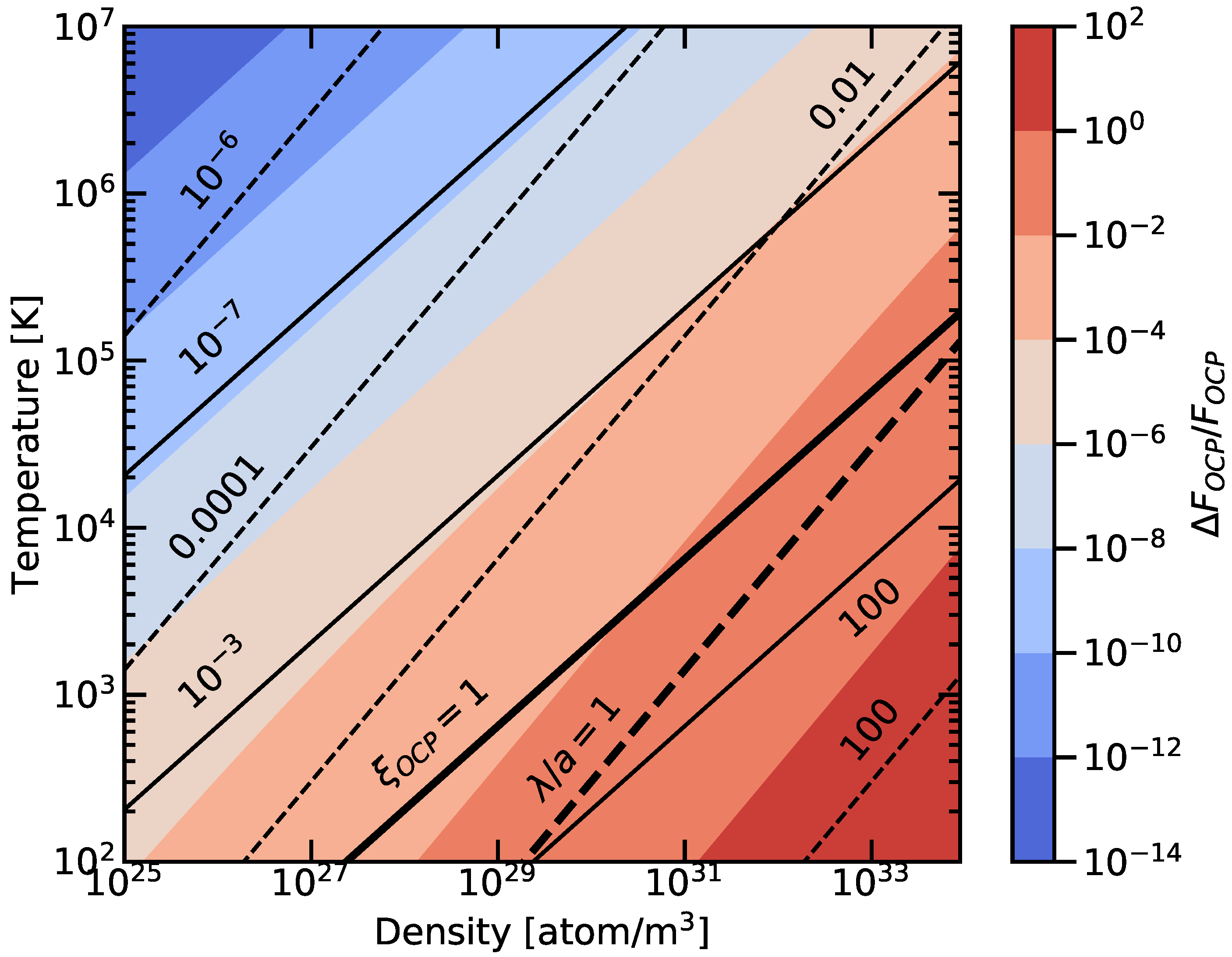
4. Application to the One-Component Plasma

As an illustration, we consider the specific case of the one-component plasma (OCP) which consists of a single species of point ions with charge $Ze$, where Z is the atomic number and e is the proton charge, immersed in a uniform neutralizing electronic background [14]. The potential energy of the system comes from the Coulombic interaction among ions and from the Coulombic interaction between ions and the neutralizing background; it can therefore be expressed by

$$V=\frac{1}{2}\sum \sum _{i\ne j=1}^N\frac{Z^2{e}^2}{4\pi {ϵ}_0\left|{\mathbf{r}}_{\mathbf{i}}-{\mathbf{r}}_{\mathbf{j}}\right|}-{\int }_{\mathcal{V}}{n}_0\sum _{i=1}^N\frac{Z{e}^2}{4\pi {ϵ}_0\left|{\mathbf{r}}_{\mathbf{i}}-{\mathbf{r}}_{\mathbf{e}}\right|}\mathrm{d}{\mathbf{r}}_{\mathbf{e}},$$

(30)

where $n_0=NZ/\mathcal{V}$ and ${ϵ}_0$ is the dielectric permittivity of vacuum. From Equation (30), it follows that [11]

$${\langle {\nabla }_j^{2}V\rangle }_c=\frac{n_{0}Z{e}^2}{{ϵ}_0}.$$

(31)

Let ${\xi }_{OCP}$ be $\xi$ for the OCP. By using Equation (31) in Equation (28), we find

$${\xi }_{OCP}=\frac{\pi }{6}\frac{{\lambda }^2}{a^2}{\mathsf{\Gamma }}_{OCP},$$

(32)

where ${\alpha }_3=-1/24$ has been taken into account and where

$${\mathsf{\Gamma }}_{OCP}=\beta \frac{Z^2{e}^2}{4\pi {ϵ}_{0}a},$$

(33)

is the usual definition of the coupling constant in the OCP. As interpreted above, ${\xi }_{OCP}$ is proportional to the coupling constant. This expression of ${\xi }_{OCP}$ is identical to that found in the literature and expressed as [14,15,16]

$${\xi }_{OCP}=\frac{1}{24}{(\beta \hslash {\omega }_p)}^2,$$

(34)

where ${\omega }_p$ is the plasma frequency defined by

$${\omega }_p^2=\frac{N}{\mathcal{V}}\frac{Z^2{e}^2}{{ϵ}_{0}m}.$$

(35)

It is worth noting that, in Ref. [15], the authors also derive the ${\lambda }^4/a^4$ term in an explicit form for both the liquid and solid one-component plasmas. The quantum correction is dependent on ${\lambda }^2/a^2$ but also on the relative intensity of the potential energy compared to the kinetic energy. To illustrate the importance of the potential, we plotted in Figure 1 the evolution of the quantum correction to the free energy for a fully ionized hydrogen plasma (an OCP) as a function of density and temperature. The quantum corrections are of course very small at low density and high temperature but become the dominant contribution to the free energy at low temperature and high density. There, they cannot be considered as “corrections” anymore. On this graph it is clear that the evolution of the quantum correction is the same as that of the ${\xi }_{\mathrm{OCP}}$ parameter at high temperature and low density. However, the $\lambda /a$ ratio does not reproduce the density-temperature dependence of the quantum correction. It is thus clear that the “$\hslash \to 0$ limit” generally evoked is actually a “$\xi \to 0$ limit”.

5. Conclusions

In the framework of Boltzmann statistics, we have revisited the ${\hslash }^2$ expansion of the partition function and of the free energy by using simple calculations. We have shown that, in a dimensionless form, the expansion of the free energy is equivalent to an expansion in ${\lambda }^2/a^2$ whose coefficients are dimensionless functionals of the potential energy (divided by $k_{B}T$) depending on no parameter. These coefficients depend in particular (but not only) on the typical length of variation of the potential.

By retaining the first-order corrective term of the expansion in ${\lambda }^2/a^2$ to evaluate the quantum correction, the latter turns out to be characterized by a dimensionless parameter proportional to the product of ${\lambda }^2/a^2$ by an effective coupling constant, as shown in Equation (28). As an illustration, the characteristic parameter of the OCP is considered; then the effective coupling constant is proportional to the coupling constant usually defined, as shown in Equation (32). In order to properly evaluate the intensity of the quantum correction, it is thus necessary to consider not only temperature and density but also the magnitude of the potential in which the particles evolve.

An extreme case is that of the ideal gas. Since there is no interaction among atoms, the operators $\widehat{K}$ and $\widehat{V}$ trivially commute so that there is no quantum correction under the assumptions of this work, and this for any thermal de Broglie wavelength. However, the fermion or boson exchange effects between particles, which have been assumed to be negligible in the present work, must now be taken into account in the calculation of the quantum correction; for an ideal gas, the latter varies like ${\lambda }^3/a^3$ for small values of $\lambda /a$ [7].

As indicated in the introduction, the main purpose of this work is of a didactic nature. Other approaches allow to obtain the same results. One of them is to deduce w from the identity of the right-hand sides of Equations (9) and (10). Another approach is to consider the Laplace transform of the matrix elements involved in the calculation of Q and to obtain an ℏ expansion of the resulting resolvant of the operator $\widehat{H}$ [11]. For obtaining the general form of the ℏ expansion of Q and of its coefficients, we have found these two approaches to be much more tedious than the one presented in this work.

References

1. Becca, F.; Sorella, S. Quantum Monte Carlo Approaches for Correlated Systems; Cambridge University Press: Cambridge, UK, 2017. [Google Scholar]
2. Geneste, G.; Torrent, M.; Bottin, F.; Loubeyre, P. Strong Isotope Effect in Phase II of Dense Solid Hydrogen and Deuterium. Phys. Rev. Lett. 2012, 109, 155303. [Google Scholar] [CrossRef] [PubMed] [Green Version]
3. Clérouin, J.; Recoules, V.; Soubiran, F. The advent of ab initio simulations of dense plasmas. Contrib. Plasma Phys. 2021, 61, e202100095. [Google Scholar] [CrossRef]
4. Ceperley, D.M. Path Integral Monte Carlo Methods for Fermions. In Monte Carlo and Molecular Dynamics of Condensed Matter Systems; Binder, K., Ciccotti, G., Eds.; Editrice Compositori: Bologna, Italy, 1996. [Google Scholar]
5. Militzer, B.; González-Cataldo, F.; Zhang, S.; Driver, K.; Soubiran, F. First-principles equation of state database for warm dense matter computation. Phys. Rev. E 2021, 103, 013203. [Google Scholar] [CrossRef] [PubMed]
6. Saumon, D.; Starrett, C.E. Pseudo-atom molecular dynamics: A model for warm and hot dense matter. AIP Conf. Proc. 2020, 2272, 090002. [Google Scholar]
7. McQuarrie, D.A. Statistical Mechanics; University Science Books: Sausalito, CA, USA, 2000. [Google Scholar]
8. Wigner, E. On the Quantum Correction For Thermodynamic Equilibrium. Phys. Rev. 1932, 40, 749. [Google Scholar] [CrossRef]
9. Kirkwood, J.G. Quantum Statistics of Almost Classical Assemblies. Phys. Rev. 1933, 44, 31. [Google Scholar] [CrossRef]
10. Brack, M.; Bhaduri, R.K. Semiclassical Physics; CRC Press: Boca Raton, FL, USA, 2003. [Google Scholar]
11. Samaj, L.; Jancovici, B. Wigner Kirkwood expansion for semi-infinite quantum fluids. J. Stat. Mech. 2007, 2007, P02002. [Google Scholar] [CrossRef] [Green Version]
12. Jizba, P.; Zatloukal, V. Path-integral approach to the Wigner-Kirkwood expansion. Phys. Rev. E 2014, 89, 012135. [Google Scholar] [CrossRef] [PubMed] [Green Version]
13. DeWitt, H.E. Analytic properties of the quantum corrections to the second virial coefficient. J. Math. Phys. 1962, 3, 1003. [Google Scholar] [CrossRef]
14. Hansen, J.-P. Statistical Mechanics of Dense Ionized Matter. I. Equilibrium Properties of the Classical One-Component Plasma. Phys. Rev. A 1973, 8, 3096. [Google Scholar] [CrossRef]
15. Hansen, J.P.; Vieillefosse, P. Quantum corrections in dense ionized matter. Phys. Lett. 1975, 53, 188. [Google Scholar] [CrossRef]
16. Chabrier, G.; Mazevet, S.; Soubiran, F. A New Equation of State for Dense Hydrogen–Helium Mixtures. Astrophys. J. 2019, 51, 872. [Google Scholar] [CrossRef] [Green Version]
17. Chabrier, G.; Potekhin, A.Y. Equation of state of fully ionized electron-ion plasmas. Phys. Rev. B 1998, 58, 4941. [Google Scholar] [CrossRef] [Green Version]
18. Potekhin, A.Y.; Chabrier, G. Thermodynamic Functions of Dense Plasmas: Analytic Approximations for Astrophysical Applications. Contrib. Plasma Phys. 2010, 50, 82. [Google Scholar] [CrossRef] [Green Version]
Figure 1. Temperature-density dependence of the first corrective term Δ F O C P in the Wigner-Kirkwood expansion of the free energy in the OCP approximation for a fully ionized hydrogen plasma. The OCP free energy F OCP corresponds to the ionic classical contribution as defined in Refs. [17,18]. The full lines correspond to iso-values of the parameter ξ OCP and the dashed lines represent iso-values of λ / a .
Atoms 10 00065 g001
Publisher’s Note: MDPI stays neutral with regard to jurisdictional claims in published maps and institutional affiliations.