
Calculation of Low-Lying Electronic Excitations of Magnesium Monofluoride: How Well Do Coupled-Cluster Methods Work?


Abstract
1. Introduction
2. Methodology
3. Results
3.1. MgF( → )
3.2. MgF( → )
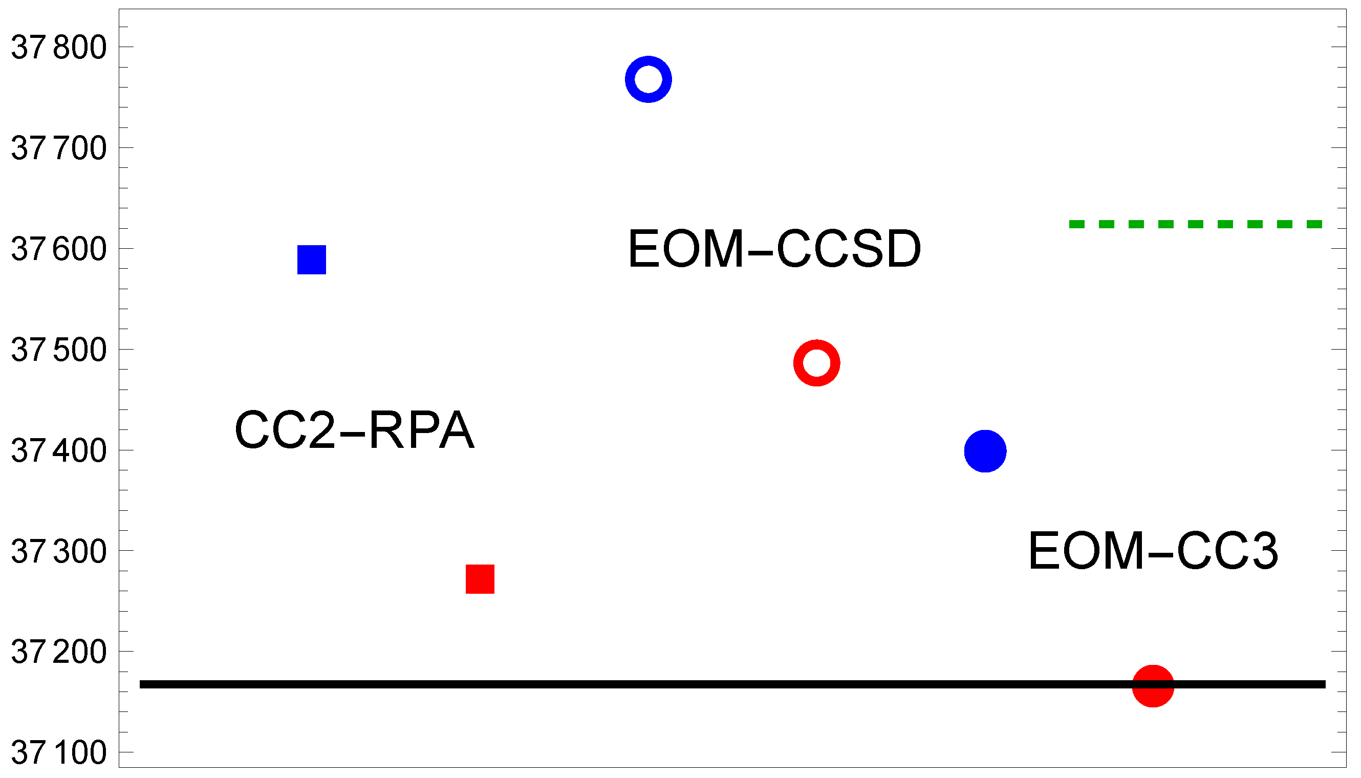
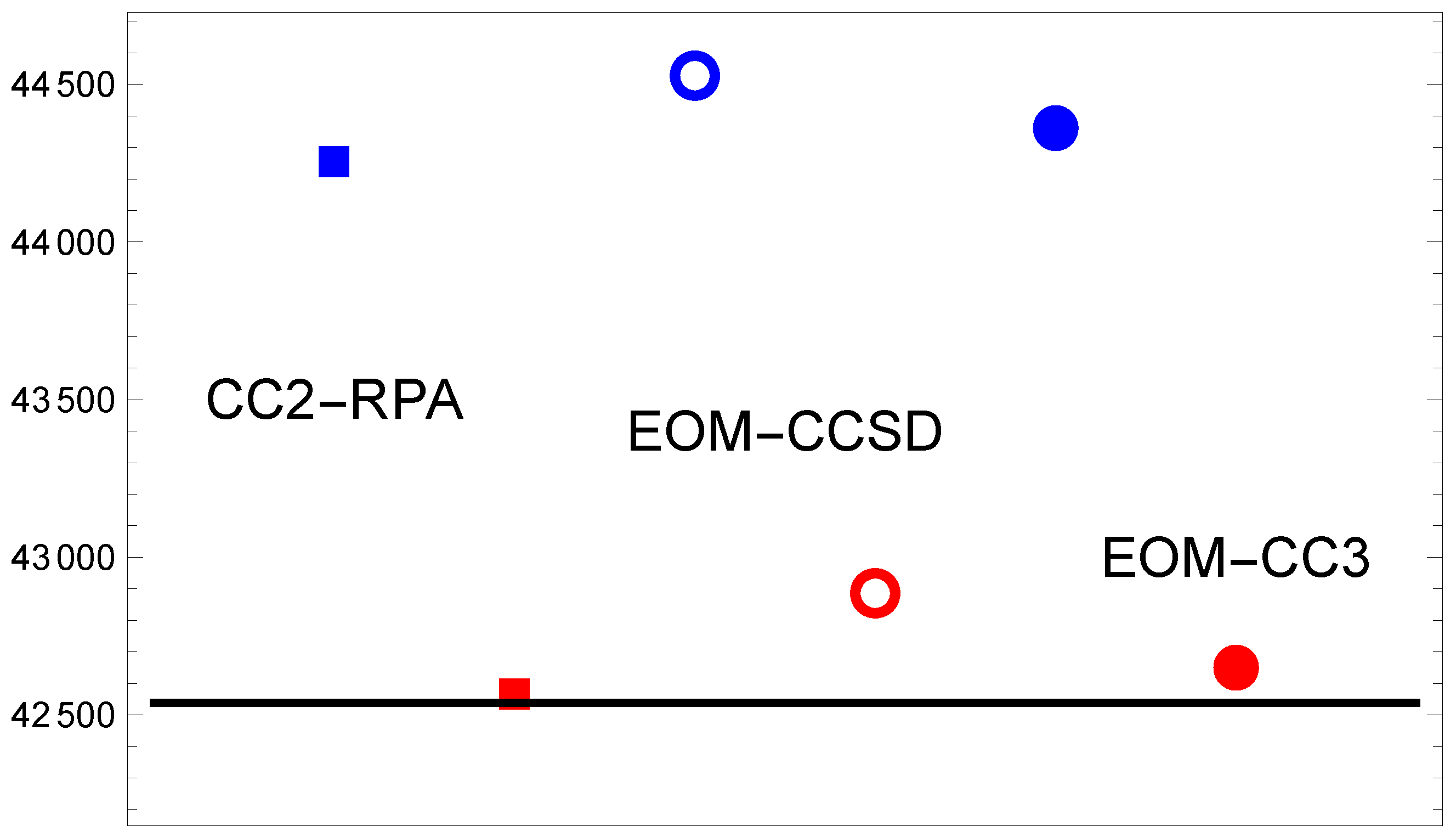
3.3. MgF( → )
4. Conclusions
Funding
Data Availability Statement
Acknowledgments
Conflicts of Interest
Appendix A

| CC2 | CC2 | CCSD | CCSD | CC3 | CC3 | ||
|---|---|---|---|---|---|---|---|
| TZ | 27,646 | 27,407 | 27,783 | 27,545 | 27,731 | 27,507 | |
| QZ | 27,673 | 27,459 | 27,828 | 27,605 | 27,758 | 27,566 | |
| 5Z | 27,634 | 27,798 | 27,744 | ||||
| CBS | 27,692 | 27,738 | 27,861 | 27,912 | 27,777 | 27,849 | |
| TZ | 37,637 | 37,205 | 37,785 | 37,283 | 37,426 | 36,966 | |
| QZ | 37,608 | 37,059 | 37,775 | 37,196 | 37,412 | 36,895 | |
| 5Z | 36,895 | 37,378 | 37,067 | ||||
| CBS | 37,587 | 37,270 | 37,768 | 37,486 | 37,402 | 37,169 | |
| TZ | 47,267 | 42,159 | 47,550 | 42,408 | 47,337 | 42,257 | |
| QZ | 45,521 | 42,189 | 45,803 | 42,472 | 45,625 | 42,316 | |
| 5Z | 42,316 | 42,732 | 42,534 | ||||
| CBS | 44,247 | 42,559 | 44,527 | 42,886 | 44,375 | 42,663 |
References
- Barrow, R.F.; Beale, J.R. Rotational analysis of electronic bands of gaseous MgF. Proc. Phys. Soc. 1967, 91, 483. [Google Scholar] [CrossRef]
- Novikov, M.M.; Gurvich, L.V. The electronic spectra of MgF and MgF+. J. Appl. Spectrosc. 1971, 14, 820–822. [Google Scholar] [CrossRef]
- Xu, S.; Xia, M.; Yin, Y.; Gu, R.; Xia, Y.; Yin, J. Determination of the normal A2Π state in MgF with application to direct laser cooling of molecules. J. Chem. Phys. 2019, 150, 084302. [Google Scholar] [CrossRef]
- Doppelbauer, M.; Wright, S.C.; Hofsäss, S.; Sartakov, B.G.; Meijer, G.; Truppe, S. Hyperfine-resolved optical spectroscopy of the A2Π←X2Σ+ transition in MgF. J. Chem. Phys. 2022, 156, 134301. [Google Scholar] [CrossRef] [PubMed]
- Kang, S.; Gao, Y.; Kuang, F.; Gao, T.; Du, J.; Jiang, G. Theoretical study of laser cooling of magnesium monofluoride using ab initio methods. Phys. Rev. A 2015, 91, 042511, Erratum in Phys. Rev. A 2015, 92, 069902. [Google Scholar] [CrossRef]
- Gu, J.; Xiao, Z.; Yu, C.; Zhang, Q.; Chen, Y.; Zhao, D. High resolution laser excitation spectra and Franck-Condon factors of A2Π–X2Σ+ electronic transition of MgF. Chin. J. Chem. Phys. 2022, 35, 58–68. [Google Scholar] [CrossRef]
- Hou, S.; Bernath, P.F. Line list for the MgF ground state. J. Quant. Spectrosc. Radiat. Transf. 2017, 203, 511–516. [Google Scholar] [CrossRef]
- Berning, A.; Schweizer, M.; Werner, H.J.; Knowles, P.J.; Palmieri, P. Spin-orbit matrix elements for internally contracted multireference configuration interaction wavefunctions. Mol. Phys. 2000, 98, 1823–1833. [Google Scholar] [CrossRef]
- Bruder, F.; Franzke, Y.J.; Weigend, F. Paramagnetic NMR Shielding Tensors Based on Scalar Exact Two-Component and Spin–Orbit Perturbation Theory. J. Phys. Chem. A 2022, 126, 5050–5069. [Google Scholar] [CrossRef] [PubMed]
- TURBOMOLE V7.8 2024, a Development of University of Karlsruhe and Forschungszentrum Karlsruhe GmbH, 1989–2007. TURBOMOLE GmbH, Since 2007. Available online: http://www.turbomole.com (accessed on 31 July 2024).
- Vutha, A.C.; Horbatsch, M.; Hessels, E.A. Oriented Polar Molecules in a Solid Inert-Gas Matrix: A Proposed Method for Measuring the Electric Dipole Moment of the Electron. Atoms 2018, 6, 3. [Google Scholar] [CrossRef]
- Buchachenko, A.A.; Viehland, L.A. Interaction potentials and transport properties of Ba, Ba+, and Ba2+ in rare gases from He to Xe. J. Chem. Phys. 2018, 148, 154304. [Google Scholar] [CrossRef] [PubMed]
- Kleshchina, N.N.; Kalinina, I.S.; Leibin, I.V.; Bezrukov, D.S.; Buchachenko, A.A. Stable axially symmetric atomic impurity in an fcc solid—Ba in rare gases. J. Chem. Phys. 2019, 151, 121104. [Google Scholar] [CrossRef] [PubMed]
- Koyanagi, G.K.; Lambo, R.L.; Ragyanszki, A.; Fournier, R.; Horbatsch, M.; Hessels, E.A. Accurate calculation of the interaction of a barium monofluoride molecule with an argon atom: A step towards using matrix isolation of BaF for determining the electron electric dipole moment. J. Mol. Spectrosc. 2023, 391, 111736. [Google Scholar] [CrossRef]
- Lambo, R.L.; Koyanagi, G.K.; Ragyanszki, A.; Horbatsch, M.; Fournier, R.; Hessels, E.A. Calculation of the local environment of a barium monofluoride molecule in an argon matrix: A step towards using matrix-isolated BaF for determining the electron electric dipole moment. Mol. Phys. 2023, 121, e2198044. [Google Scholar] [CrossRef]
- Lambo, R.L.; Koyanagi, G.K.; Horbatsch, M.; Fournier, R.; Hessels, E.A. Calculation of the local environment of a barium monofluoride molecule in a neon matrix. Mol. Phys. 2023, 121, e2232051. [Google Scholar] [CrossRef]
- Hao, Y.; Pašteka, L.F.; Visscher, L.; Aggarwal, P.; Bethlem, H.L.; Boeschoten, A.; Borschevsky, A.; Denis, M.; Esajas, K.; Hoekstra, S.; et al. High accuracy theoretical investigations of CaF, SrF, and BaF and implications for laser-cooling. J. Chem. Phys. 2019, 151, 034302. [Google Scholar] [CrossRef] [PubMed]
- Skripnikov, L.V.; Chubukov, D.V.; Shakhova, V.M. The role of QED effects in transition energies of heavy-atom alkaline earth monofluoride molecules: A theoretical study of Ba+, BaF, RaF, and E120F. J. Chem. Phys. 2021, 155, 144103. [Google Scholar] [CrossRef] [PubMed]
- Kyuberis, A.A.; Pašteka, L.F.; Eliav, E.; Perrett, H.A.; Sunaga, A.; Udrescu, S.M.; Wilkins, S.G.; Garcia Ruiz, R.F.; Borschevsky, A. Theoretical determination of the ionization potentials of CaF, SrF, and BaF. Phys. Rev. A 2024, 109, 022813. [Google Scholar] [CrossRef]
- Denis, M.; Haase, P.A.B.; Mooij, M.C.; Chamorro, Y.; Aggarwal, P.; Bethlem, H.L.; Boeschoten, A.; Borschevsky, A.; Esajas, K.; Hao, Y.; et al. Benchmarking of the Fock-space coupled-cluster method and uncertainty estimation: Magnetic hyperfine interaction in the excited state of BaF. Phys. Rev. A 2022, 105, 052811. [Google Scholar] [CrossRef]
- Norrgard, E.B.; Chamorro, Y.; Cooksey, C.C.; Eckel, S.P.; Pilgram, N.H.; Rodriguez, K.J.; Yoon, H.W.; Pašteka, L.F.; Borschevsky, A. Radiative decay rate and branching fractions of MgF. Phys. Rev. A 2023, 108, 032809. [Google Scholar] [CrossRef]
- Hättig, C.; Weigend, F. CC2 excitation energy calculations on large molecules using the resolution of the identity approximation. J. Chem. Phys. 2000, 113, 5154–5161. [Google Scholar] [CrossRef]
- Hättig, C. Structure Optimizations for Excited States with Correlated Second-Order Methods: CC2 and ADC(2). In Response Theory and Molecular Properties (A Tribute to Jan Linderberg and Poul Jørgensen); Jensen, H., Ed.; Advances in Quantum Chemistry; Academic Press: Cambridge, MA, USA, 2005; Volume 50, pp. 37–60. [Google Scholar] [CrossRef]
- Weigend, F.; Ahlrichs, R. Balanced basis sets of split valence, triple zeta valence and quadruple zeta valence quality for H to Rn: Design and assessment of accuracy. Phys. Chem. Chem. Phys. 2005, 7, 3297–3305. [Google Scholar] [CrossRef] [PubMed]
- Hättig, C.; Köhn, A. Transition moments and excited-state first-order properties in the coupled-cluster model CC2 using the resolution-of-the-identity approximation. J. Chem. Phys. 2002, 117, 6939–6951. [Google Scholar] [CrossRef]
- Gauss, J. Equation-of-Motion Coupled-Cluster Theory, 2017. Available online: https://www.esqc.org/lectures/gauss_EOM_lecture_handout.pdf (accessed on 31 May 2024).
- Crawford, T.D.; Schaefer, H.F., III. An Introduction to Coupled Cluster Theory for Computational Chemists. In Reviews in Computational Chemistry; John Wiley & Sons, Ltd.: Hoboken, NJ, USA, 2000; pp. 33–136. [Google Scholar] [CrossRef]
- Smith, D.G.A.; Burns, L.A.; Simmonett, A.C.; Parrish, R.M.; Schieber, M.C.; Galvelis, R.; Kraus, P.; Kruse, H.; Di Remigio, R.; Alenaizan, A.; et al. PSI4 1.4: Open-source software for high-throughput quantum chemistry. J. Chem. Phys. 2020, 152, 184108. [Google Scholar] [CrossRef]
- Loos, P.F.; Scemama, A.; Blondel, A.; Garniron, Y.; Caffarel, M.; Jacquemin, D. A Mountaineering Strategy to Excited States: Highly Accurate Reference Energies and Benchmarks. J. Chem. Theory Comput. 2018, 14, 4360–4379. [Google Scholar] [CrossRef] [PubMed]
- Damour, Y.; Quintero-Monsebaiz, R.; Caffarel, M.; Jacquemin, D.; Kossoski, F.; Scemama, A.; Loos, P.F. Ground- and Excited-State Dipole Moments and Oscillator Strengths of Full Configuration Interaction Quality. J. Chem. Theory Comput. 2023, 19, 221–234. [Google Scholar] [CrossRef] [PubMed]
- Paul, A.C.; Myhre, R.H.; Koch, H. New and Efficient Implementation of CC3. J. Chem. Theory Comput. 2021, 17, 117–126. [Google Scholar] [CrossRef] [PubMed]
- Damour, Y.; Scemama, A.; Jacquemin, D.; Kossoski, F.; Loos, P.F. State-Specific Coupled-Cluster Methods for Excited States. J. Chem. Theory Comput. 2024, 20, 4129–4145. [Google Scholar] [CrossRef] [PubMed]
- Lee, J.; Small, D.W.; Head-Gordon, M. Excited states via coupled cluster theory without equation-of-motion methods: Seeking higher roots with application to doubly excited states and double core hole states. J. Chem. Phys. 2019, 151, 214103. [Google Scholar] [CrossRef]
- Prascher, B.P.; Woon, D.E.; Peterson, K.A.; Dunning, T.H.; Wilson, A.K. Gaussian basis sets for use in correlated molecular calculations. VII. Valence, core-valence, and scalar relativistic basis sets for Li, Be, Na, and Mg. Theor. Chem. Accounts 2011, 128, 69–82. [Google Scholar] [CrossRef]
- Kendall, R.A.; Dunning, T.H., Jr.; Harrison, R.J. Electron affinities of the first-row atoms revisited. Systematic basis sets and wave functions. J. Chem. Phys. 1992, 96, 6796–6806. [Google Scholar] [CrossRef]
- Peterson, K.A.; Woon, D.E.; Dunning, T.H., Jr. Benchmark calculations with correlated molecular wave functions. IV. The classical barrier height of the H+H2→ H2+H reaction. J. Chem. Phys. 1994, 100, 7410–7415. [Google Scholar] [CrossRef]
- Bernath, P.F. Spectra of Atoms and Molecules, 4th ed.; Oxford University Press: Oxford, UK, 2020. [Google Scholar]
- Linstrom, P.J.; Mallard, W.G. NIST Chemistry WebBook, NIST Standard Reference Database Number 69; National Institute of Standards and Technology: Gaithersburg, MD, USA, 2023. [CrossRef]
- Field, R.W.; Bergeman, T.H. Radio-Frequency Spectroscopy and Perturbation Analysis in CS A1Π(υ = 0). J. Chem. Phys. 1971, 54, 2936–2948. [Google Scholar] [CrossRef]


| (Expt) | EOM-CCSD | CCSD(T) | CC3 | ||
|---|---|---|---|---|---|
| 712 | 1.7500 | 1.735 | 1.740 | 1.742 | |
| [740, 746] | 1.7469 | 1.717 | |||
| 751 | 1.7185 | 1.699 | |||
| 813 | 1.6988 | 1.677 |
| CBS | Expt | ||||
|---|---|---|---|---|---|
| 27,507 | 27,556 | 27,744 | 27,849 | 27,817 27,834 † | |
| 36,966 | 36,895 | 37,067 | 37,169 | 37,167 | |
| 42,257 | 42,316 | 42,534 | 42,663 | 42,590 |
Disclaimer/Publisher’s Note: The statements, opinions and data contained in all publications are solely those of the individual author(s) and contributor(s) and not of MDPI and/or the editor(s). MDPI and/or the editor(s) disclaim responsibility for any injury to people or property resulting from any ideas, methods, instructions or products referred to in the content. |
© 2024 by the author. Licensee MDPI, Basel, Switzerland. This article is an open access article distributed under the terms and conditions of the Creative Commons Attribution (CC BY) license (https://creativecommons.org/licenses/by/4.0/).
Share and Cite
Horbatsch, M. Calculation of Low-Lying Electronic Excitations of Magnesium Monofluoride: How Well Do Coupled-Cluster Methods Work? Atoms 2024, 12, 40. https://doi.org/10.3390/atoms12080040
Horbatsch M. Calculation of Low-Lying Electronic Excitations of Magnesium Monofluoride: How Well Do Coupled-Cluster Methods Work? Atoms. 2024; 12(8):40. https://doi.org/10.3390/atoms12080040
Chicago/Turabian StyleHorbatsch, Marko. 2024. "Calculation of Low-Lying Electronic Excitations of Magnesium Monofluoride: How Well Do Coupled-Cluster Methods Work?" Atoms 12, no. 8: 40. https://doi.org/10.3390/atoms12080040
APA StyleHorbatsch, M. (2024). Calculation of Low-Lying Electronic Excitations of Magnesium Monofluoride: How Well Do Coupled-Cluster Methods Work? Atoms, 12(8), 40. https://doi.org/10.3390/atoms12080040