Abstract
We discuss an extension of the Single-Active-Electron (SAE) approximation in atoms by allowing the model potential to depend on the angular-momentum quantum number ℓ. We refer to this extension as the ℓ-SAE approximation. The main ideas behind ℓ-SAE are illustrated using the helium atom as a benchmark system. We show that introducing ℓ-dependent potentials improves the accuracy of key quantities in atomic structure computed from the Time-Independent Schrödinger Equation (TISE), including energies, oscillator strengths, and static and dynamic polarizabilities, compared to the standard SAE approach. Additionally, we demonstrate that the ℓ-SAE approximation is suitable for quantum simulations of light−atom interactions described by the Time-Dependent Schrödinger Equation (TDSE). As an illustration, we simulate High-order Harmonic Generation (HHG) and the three-sideband (3SB) version of the Reconstruction of Attosecond Beating by Interference of Two-photon Transitions (RABBITT) technique, achieving enhanced accuracy comparable to that obtained in all-electron calculations. One of the main advantages of the ℓ-SAE approach is that existing SAE codes can be easily adapted to handle ℓ-dependent potentials without any additional computational cost.
1. Introduction
The Single-Active-Electron (SAE) approximation is a major tool for simulating photoinduced processes in the nonlinear regime of light−atom interactions.1 By providing a simplified description of the atomic system, it offers a framework for efficiently solving the Time-Dependent Schrödinger Equation (TDSE) with high accuracy. According to the principle behind the SAE approximation, the atom of interest is treated as a core plus one active electron, which is typically weakly bound. The core, made up of electrons and the nucleus, is assumed to be frozen, with its electric charge spherically distributed. Thus, the quantum dynamics of the system under the influence of a laser field are governed by the active electron. This simplified picture of the atomic system provided by the SAE approximation can describe the physics of multiphoton single-ionization and, more generally, multiphoton processes involving one-electron transitions, as long as correlation effects are small. In practice, the SAE approximation stands out due to its low computational cost and its ability to capture both the qualitative and quantitative aspects of the underlying physical processes. That is why it has been extensively employed to establish benchmark calculations before running multi-electron codes [1,2,3,4,5,6].
The interaction between the core and the active electron is described by a radial/central model potential. In general, there are two approaches for constructing such models: (i) interpolating the potential directly from ab initio calculations, such as Kohn–Sham density functional theory [7] or Hartree–Slater considerations [8,9,10], and (ii) fitting the potential to reproduce a selected set of experimental, or reference, bound-state energies, e.g., [11,12]. Once the model potential is defined, the accuracy of the SAE energy levels becomes crucial in quantum simulations. This accuracy plays a major role when multiphoton resonant transitions between bound states occur during light−atom interactions. For example as noted in [13], an error of a few percent in the SAE atom’s ground-state energy can result in an error of several hundred percent in multiphoton ionization rates.
To improve the agreement between SAE energy levels and experimental/reference values, we can take advantage of the radial character of the model potential by making it ℓ-dependent.2 We call this the ℓ-SAE approximation. Within the framework of the Time-Independent Schrödinger Equation (TISE), this approach has already been used successfully for the description of the bound states of alkali atoms [12,15,16,17,18], as well as in subsequent collision calculations, e.g., [19,20,21,22]. A general scheme to tackle, in principle, any atom was presented in [8] in the context of the Hartree–Fock–Slater method. In contrast, to the best of our knowledge, ℓ-dependent potentials have rarely been used in TDSE-based simulations. Although the idea behind the ℓ-SAE approximation is hinted at [23], it has only been applied to cesium to study High-order Harmonic Generation near and below the threshold [24]. For this atom, the ℓ-dependent potential was constructed based on the energies, but the accuracy of other TISE-based physical properties was not investigated.
The principal goal of the present work is to demonstrate that the ℓ-SAE approximation not only improves the agreement between experimental energies and the ℓ-SAE values but also enhances the accuracy of relevant properties/observables in the context of light−atom interactions. For concreteness, and due to its experimental relevance, we use the helium atom as a prime example. Interestingly, several ℓ-independent SAE model potentials for helium can be found in the literature [7,13,25,26,27,28,29,30]. However, to the best of our knowledge, no ℓ-dependent model for helium has been reported. While our focus is on a particular atom, it is important to note that the ℓ-SAE approximation is particularly effective for the alkali targets mentioned above, but it can reasonably be expected to also be appropriate for light quasi-two-electron atoms such as beryllium and the other alkaline-earth elements, whose structure is well described within the -coupling scheme.
This manuscript is organized as follows. We begin by constructing an ℓ-dependent model potential for helium in Section 2. Then, we investigate the accuracy of the model by calculating various atomic properties based on the TISE, with the corresponding results presented in Section 3. In Section 4, we use the ℓ-SAE approximation in time-dependent simulations to obtain results on HHG and 3SB-RABBITT. Whenever possible, we compare our results with reference values from the literature, including standard SAE approaches and other methods that account for correlation effects.
Unless stated otherwise, atomic units (a.u.) are used throughout this manuscript.
2. Potentials for Helium in the ℓ-SAE Approximation
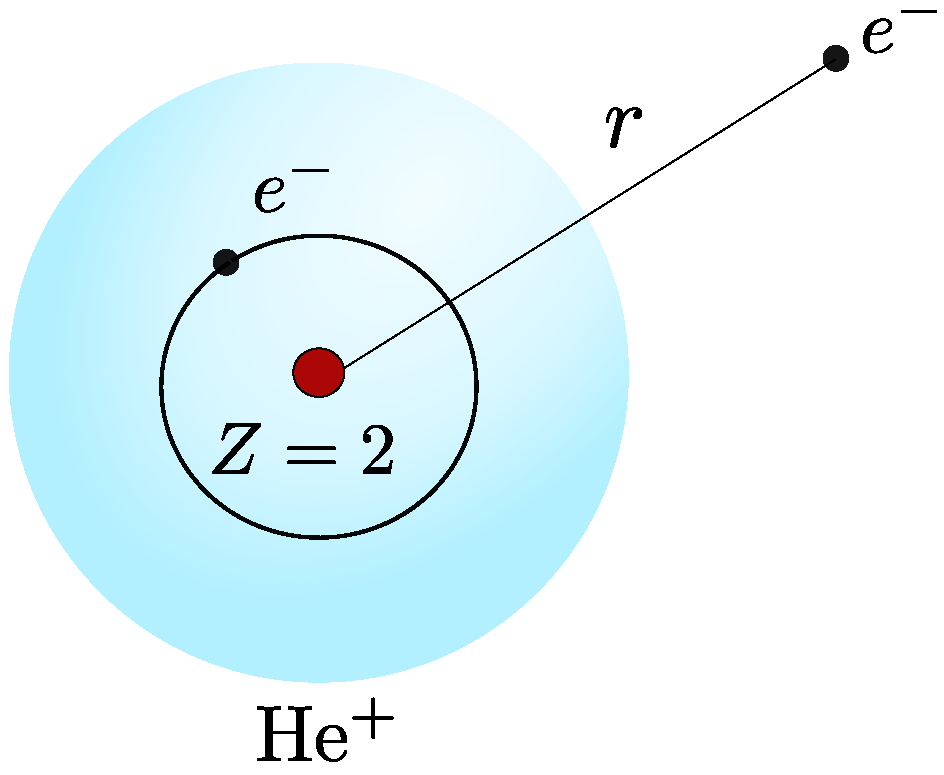
The ℓ-SAE approximation applied to the helium atom offers a suitable framework for a proof of principle beyond quasi-one-electron alkali targets, since helium is well described within the -coupling scheme with a tightly-bound inner electron (see Figure 1). In particular, the excited bound states can be labeled by in a non-relativistic treatment.3 Therefore, the energies can be grouped according to and the total spin S. In this work, we focus on the spin-singlet states, . However, the approach to tackle triplet states is similar.
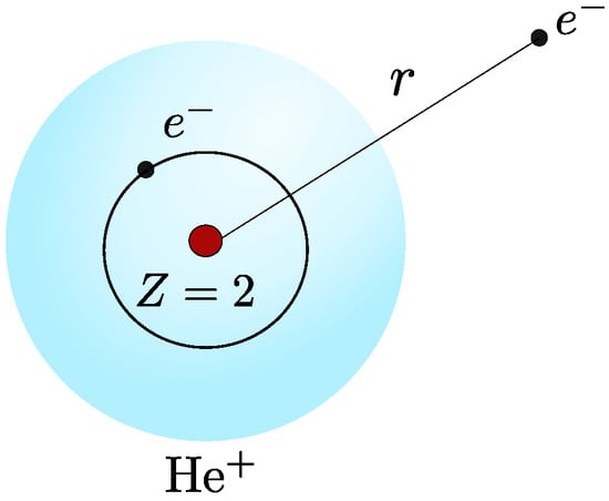
Figure 1.
Helium atom within the ℓ-SAE framework, where the interaction potential between the core (He+) and the active electron is assumed to depend on ℓ.
In the ℓ-SAE approximation, the radial part of the bound-state wavefunction of the active electron, labeled by , is determined from the reduced radial Schödinger equation
Here, is the model potential for a given ℓ. In particular, we consider
where is a set of free ℓ-dependent parameters to be determined. This model potential exhibits the required asymptotic behavior at both small and large r, namely,
and
To ensure that has infinitely many bound states, the conditions and are imposed. To optimize the value of the parameters for fixed ℓ, we minimize the weighted sum
where is a weight factor for the state (). Additionally, denotes the energy obtained from the numerical solution of Equation (1), with as given in (2). In turn, denotes the recommended values of the spin-singlet energy taken from the NIST database [31]. Therefore, W in (4) represents the weighted sum of the relative errors over a selected number of bound states, and its minimization determines the optimal configuration of the free parameters. Specifically, we considered the lowest five bound states from the series for each value of ℓ. The weights are chosen manually to uniformly maximize the number of exact digits in energies .
An accurate determination and minimization of (4) requires accurate values for . In our FORTRAN implementation, they were obtained by means of the Lagrange Mesh Method (LMM), as described in [32], which is a highly accurate approximate variational method that discretizes the equation on a non-uniform grid. This ultimately leads to the diagonalization of the discretized Hamiltonian matrix. The LMM used in this work, whose implementation is based on [33], was then coupled to the MINUIT subroutine [34] to carry out the minimization of . Due to the small number of grid points that LMM requires (∼200), combined with the high efficiency of MINUIT, the minimization procedure is fast and computationally inexpensive. Increasing the grid size beyond 200 points did not significantly change the results within double precision.
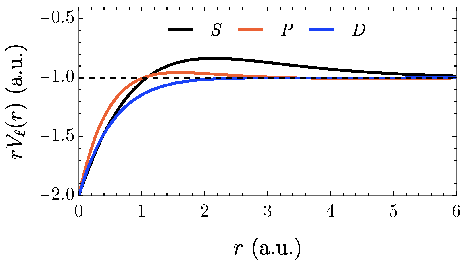
Table 1 shows the optimal parameters. The coefficients for are assumed to be the same since the centrifugal barrier, together with the Coulomb term , mainly determines the energies with high accuracy. For this reason, the coefficient was optimized for and kept fixed for non-S states. A plot of the potentials , multiplied by r, is shown in Figure 2 for . Noticeable differences can be observed, especially at intermediate distances . Of particular interest is the fact that is clearly larger than for the S and P Rydberg series. This would be impossible for purely screening one nuclear charge by the inner electron. However, the potentials also account for the exchange integral, which represents a repulsive effect for the singlet series.

Table 1.
Optimal parameters for the potentials of Equation (2), designed for the singlet states of helium.
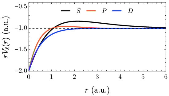
Figure 2.
Model potentials (multiplied by r) with optimized parameters for the states with (S), (P), and (D).
In our model, the ionization potential is according to . Meanwhile, the recommended value is [31]. Thus, there is a discrepancy of a.u. In Table 2, we present the energies for the first ten low-lying states of helium. For these levels, the maximum deviation is a.u., which is found for the state and represents a 0.002% error. It is well known that this state is notoriously difficult to describe also by ab initio methods [35].
Table 2.
Helium energy levels for selected low-lying spin-singlet states with . Both reference (NIST) and ℓ-SAE energies are rounded to the number of digits shown.
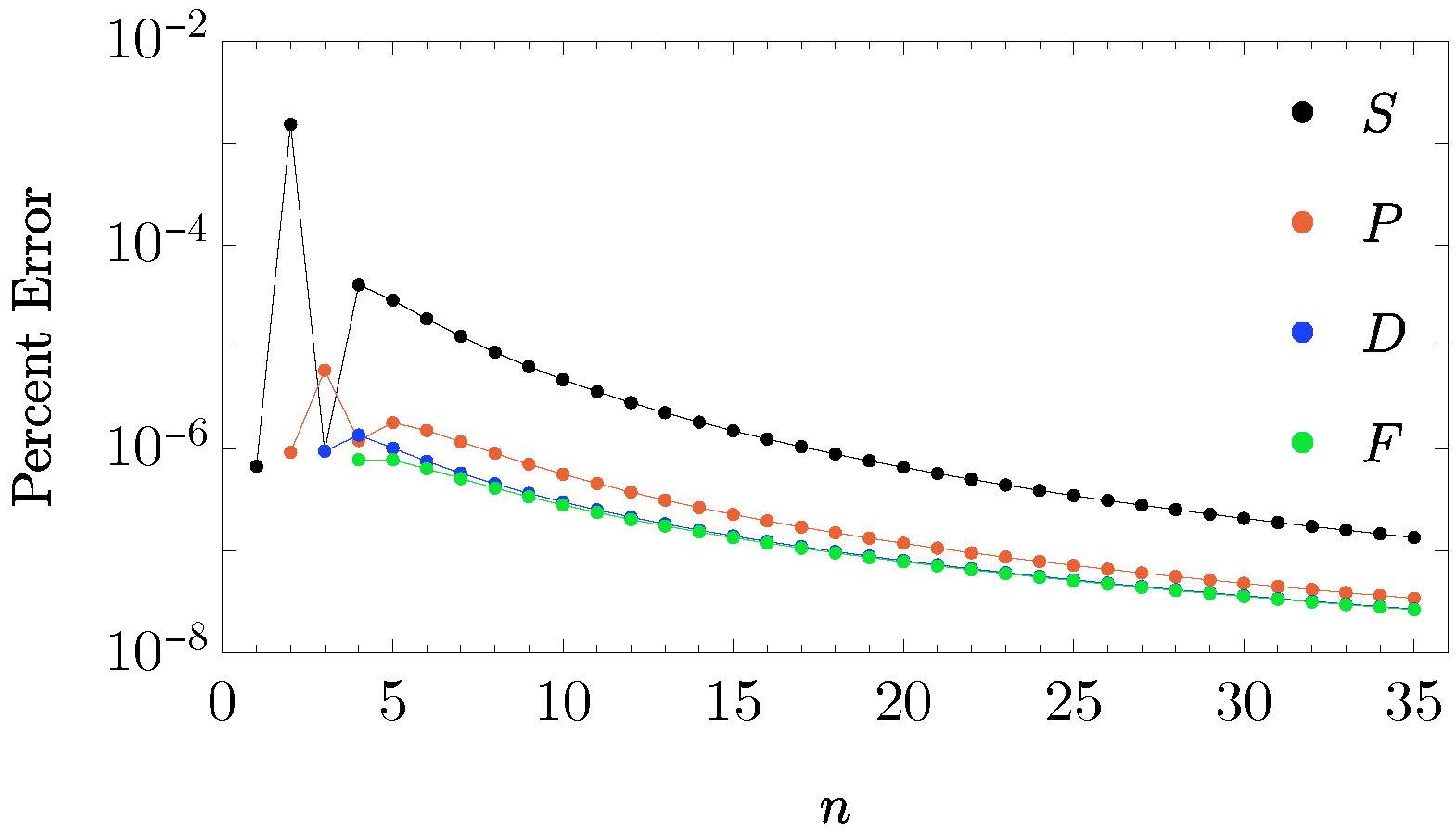
We also investigated the accuracy of the ℓ-SAE energies for the Rydberg S, P, D, and F series up to , the largest value for which reference values are available in the NIST database. As seen in Figure 3, the percent error smoothly decreases for for each series.
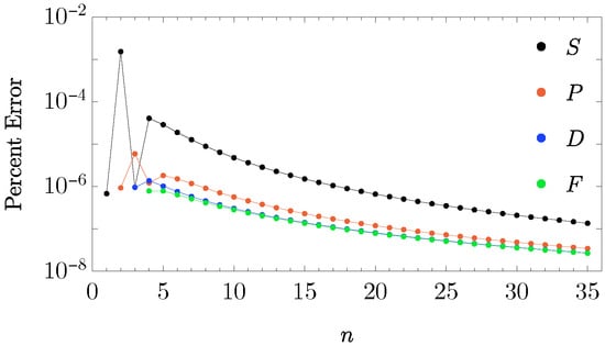
Figure 3.
Percent error of the first four Rydberg series with . In the D and F series, the errors overlap for .
For the purposes of the present work, the accuracy in energies provided by the potentials is sufficient to show the scope and improvement that the ℓ-SAE approximation offers. Moreover, we observed that increasing the number of free parameters4 in does not lead to a significant improvement in the accuracy of the energy levels.
By construction, the ℓ-SAE energy levels are more accurate than those from standard SAE models. For example, the deviations from the reference NIST ionization energy, based on the SAE potentials presented in [7,27,28,36], are 4.5%, 0.03%, 1.5%, and 2.4%, respectively. However, a detailed validation of the ℓ-SAE approach requires the study of other observables and relevant physical quantities. In the next section, based on the solution of the reduced radial TISE (1), we calculate some of them, especially those that are relevant in the context of light−atom interactions.
3. TISE-Based Atomic Properties
Once the functions are determined by solving (1), the wave functions of the spin-singlet bound states are given by
Here, denotes the familiar spherical harmonic of degree ℓ and order m. These wave functions can be straightforwardly extended to continuum states, specifically when the active electron has been detached from the core. They are used below to calculate observables. However, as will be shown, only the functions are relevant in practice.
3.1. Oscillator Strengths
Given two bound states, say and , we computed the averaged oscillator strength between them, which is defined by5
Here, the dipole integral is given by
See [37] for details. The selection rule, , must be considered in (6) to define the dipole-allowed transitions. For some of these transitions, the corresponding oscillator strengths are shown in Table 3 and compared with reference values from [38]. The maximum deviation reaches 13% for the transition, mostly due to the inaccuracy of the state. Overall, however, the remaining deviations are significantly smaller than those obtained with the widely used SAE potential proposed by Tong and Lin [27], which reaches almost a factor of 3 for the transition.
Table 3.
Averaged oscillator strengths for some selected dipole-allowed transitions between spin-singlet helium bound states. For each state in the first column, the first row corresponds to the results obtained in the framework of the ℓ-SAE approximation. The reference values [38] appear in the second row. All numbers are rounded to the digits displayed.
3.2. Static and Dynamic Polarizabilities
We now investigate the ℓ-SAE predictions for the so-called static and dynamic polarizabilities defined by
and
respectively. The summations in (8a) and (8b) are carried out over both bound and continuum states. In (8b), is the frequency that characterizes a monochromatic (thus infinitely long) laser field interacting with the atom.
Our ℓ-SAE model generally yields polarizabilities smaller than the reference values presented in [39], which account for correlation effects, see Figure 4. For example, the static polarizability comes out as , while the reference value is , corresponding to a difference of 6%. For the dynamic case, we observed qualitative agreement for all frequencies considered, namely, . The error for the dynamic polarizability does not exceed 8% in the region . In the vicinity of , the dynamic polarizability exhibits sharp antisymmetric peaks, known as resonances. Thanks to the accurate ℓ-SAE bound-state energies (cf. Table 2), the resonance positions are well reproduced. The standard SAE approximation, due to its limited energy accuracy, is unable to accurately locate these resonances.
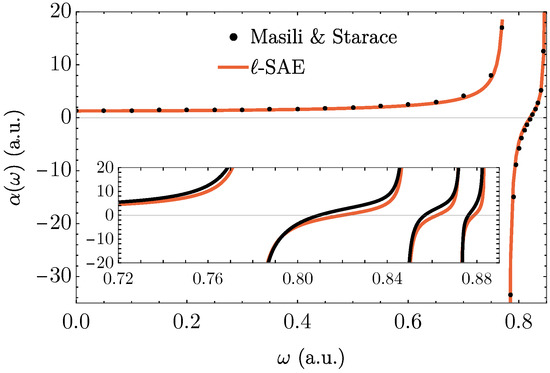
Figure 4.
Dynamic polarizability of helium as a function of . The reference data (labeled as Masili and Starace and shown in black) are given in [39]. The inset shows the region where resonances occur. The solid black curve corresponds to the digitized data from Figure 4 of [39].
3.3. Photoionization Cross Section
Even though the ℓ-SAE approach yields improved bound-state energies, one might assume that observables without explicit dependence on them will not necessarily improve in accuracy. Calculating the photoionization cross section provides a testing ground, as it encodes the transition rate from an initial bound state to a final continuum state due to the absorption of a photon with frequency . Therefore, the energy part depends solely on the ionization potential provided by the model.
In the electric dipole approximation, the photoionization cross section is given by [40]
where denotes the energy of the released p-electron. In (9), we assume that the helium atom is initially in its ground state.
Figure 5 shows from the ℓ-SAE approximation and two SAE models for comparison. In general, the ℓ-SAE provides cross sections closer to the benchmark values than the standard SAE models. One of the SAE models we used, SAE (I), yields an accurate ionization potential a.u. [27], with an accuracy comparable to that of the ℓ-SAE model. Therefore, we conclude that our ℓ-SAE approach also improves the bound-continuum dipole matrix elements corresponding to the extension of (7), due to the enhanced accuracy of the continuum wave function that also enters in (9).
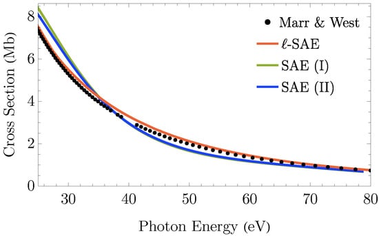
Figure 5.
Photoionization cross section (in Mb) as a function of photon energy (in eV). The reference values, labeled as Marr and West, were taken from [41]. Two predictions from the standard ℓ-independent SAE approximation with different potentials are included for comparison: SAE (I) corresponds to the potential proposed by Tong and Lin [27] for which a.u. In turn, SAE (II) corresponds to the model used in the work of Birk et al. [36] with a.u.
4. Solution of the TDSE in the ℓ-SAE Approximation
In this Section, we investigate the dynamics of the active electron within the ℓ-SAE approximation for simulations of pulsed laser−atom interactions. We limit our models to the dipole approximation and use the length gauge.
4.1. Generalities
The ℓ-SAE approach is particularly suitable when the wave function is expressed in terms of partial waves written in spherical coordinates , i.e.,
The equations governing the time evolution6 of the components are barely modified when ℓ-dependent potentials are considered: the only required modification is the replacement . Thus, standard SAE codes require minimal adjustments to implement the ℓ-SAE approximation, thereby making it particularly convenient for computational applications. In this context, we updated the SAE code described in [42] to handle ℓ-dependent potentials. Essentially, the code uses the celebrated second-order Strang splitting to propagate the initial-state wave function, typically the ground state, in time according to
where only appears in . Further technical details on the computational implementation are provided in [43]. In what follows, we consider a linearly polarized laser field. As a result, the functions , are the only contributing components in (10).
4.2. High-Order Harmonic Generation (HHG)
We consider a helium atom interacting with an intense short-pulse laser, leading to the generation of high-order harmonics. In particular, we consider the linearly-polarized laser field
where c is the speed of light, the vacuum permittivity, the laser peak intensity, N the number of optical cycles, and the (central) frequency of the driving laser. The electric field is assumed to vanish outside the time interval . We considered two sets of field parameters: (i) a.u. (248.6 nm), , W/cm2 and (ii) a.u. (1064 nm), , W/cm2. For these sets, benchmark results were recently established in the context of HHG [44].
As soon as the pulse is over, we calculate the spectral density, which represents the dipole-radiated energy per frequency . It is given by [45]
Here, is the second derivative with respect to the time of the induced dipole moment . Below, we compare our induced dipole moment and its spectral density with the results reported in [44], especially those coming from a standard SAE model and the RMT code [2], which accounts for both multi-electron and multi-channel dynamics.
4.2.1. Induced Dipole Moment
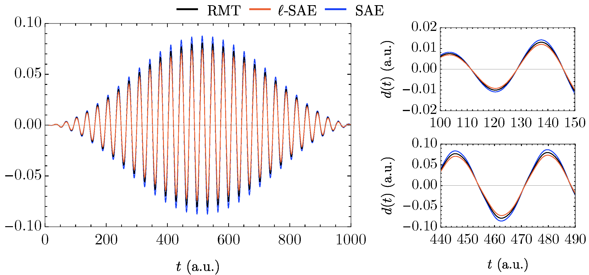
For both sets of field parameters, (i) and (ii), the corresponding dipole moment is shown in Figure 6 and Figure 7, respectively. The reference results from RMT and the SAE approximation are also included. In general, we observe that the induced dipole moment predicted by our ℓ-SAE model is smaller than the reference obtained via RMT, which presumably yields the most accurate results [44]. However, this is expected, since the static polarizability in our ℓ-SAE model is 8% smaller than the actual value. In contrast, the SAE approach used in [44] predicts a slightly larger dipole moment. Despite the differences between the dipole moments, they are quite similar. In fact, the differences become more noticeable when looking at their spectral content, as discussed below.
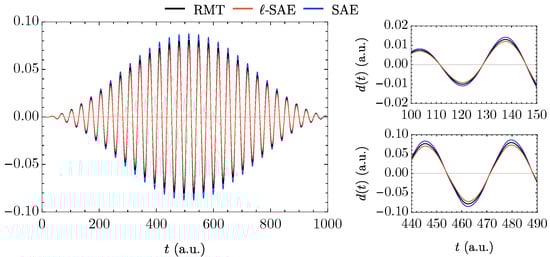
Figure 6.
Induced dipole moment as a function of time t. The results correspond to a 30-cycle laser pulse with a central wavelength of and a peak intensity of . Reference data [44], obtained using the SAE approximation and through RMT with a 6-state model, are shown.
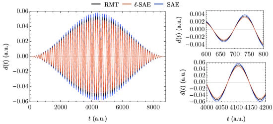
Figure 7.
Induced dipole moment as a function of time t. The results correspond to a 60-cycle pulse with a central wavelength of 1064 nm and a peak intensity of . Reference data [44], obtained using the SAE approximation and through RMT with a 3-state model, are shown.
4.2.2. Spectral Density
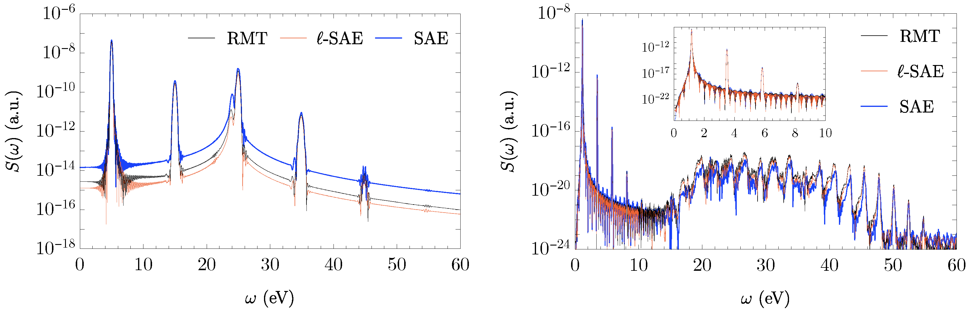
Figure 8 exhibits spectral density compared to the RMT and SAE predictions for both sets of field parameters (i) and (ii). We observe that the ℓ-SAE model captures the main features of the HHG spectra. In contrast to the SAE for set (i), the ℓ-SAE results are similar to the RMT predictions from a 6-state model. For set (ii), the ℓ-SAE results are again close to the 3-state RMT data, especially in the plateau region.
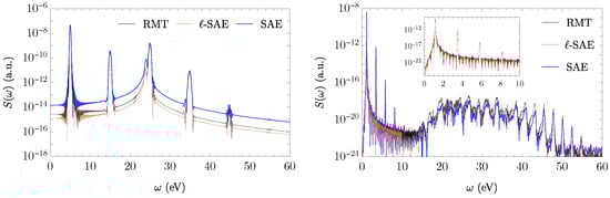
Figure 8.
Semi-log plot of the spectral density as a function of frequency , see (13). The (left panel) corresponds to a laser field with parameters (i) used in Figure 6. In this case, the predicted cutoff energy from the three-step model is approximately 34 eV, corresponding to the 7th harmonic. The (right panel), with parameters labeled by (ii) in the text and used in Figure 7, exhibits a cutoff energy at 41 eV, which is the 35th harmonic.
4.3. 3SB-RABBITT
As a final investigation, we simulated 3SB-RABBITT, a variant of 1SB-RABBITT in which the XUV comb consists of multiple odd harmonics of the frequency-doubled IR field. Consequently, the photoelectron spectrum in 3SB-RABBITT exhibits three sidebands between the main peaks, denoted as low, center, and high. For simplicity, we provide only a brief discussion of this interferometry technique, focusing on the results obtained for the observable of our interest, the RABBITT phase .
Motivated by a recent experimental realization of 3SB-RABBITT in helium [46], quantum simulations [47] were performed using the RMT code. In this approach, four different models were used in RMT: 1-, 3-, 6-, and 10-state models, representing the number of states in the close-coupling expansion. Thus, we can compare the performance of the ℓ-SAE approximation with each RMT model. In our ℓ-SAE simulations, we used the same experimentally based pulse employed in [47], which consists of a time-delayed combination of linearly polarized IR and XUV pulses with femtosecond duration. Additionally, we applied the same data-processing method as in [47].
When the time delay , given in fractions of the IR period, between the two fields is varied, the photoelectron signal at the detection angle , denoted by , oscillates according to
where A is the average signal and B is the amplitude of the oscillation. These parameters depend on the energy of the ejected electron (i.e., the specific sideband of interest) and are determined by fitting the signal to (14). To calculate , we project the wave function at the end of the pulse onto the continuum states, which are obtained for each ℓ by solving the TISE with the potential .
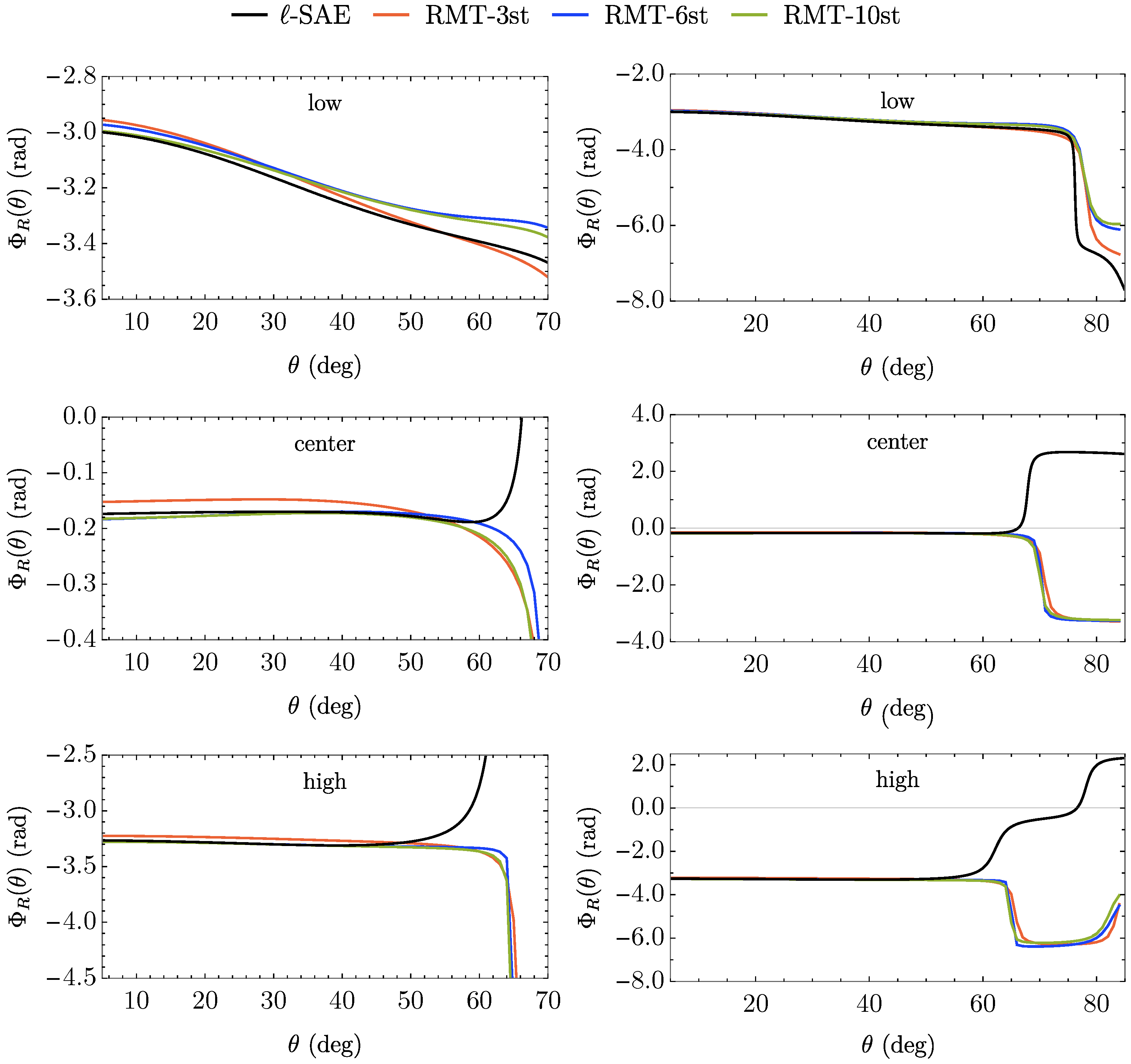
Here, we present results for the SB 14 group with an IR intensity of W/cm2. This group corresponds to three sidebands located between the energy peaks corresponding to absorption at the 13th and 15th harmonics. Similar quality in the ℓ-SAE results is observed for the other sidebands reported in [47]. Figure 9 shows the phase for the low, center, and high SBs from the ℓ-SAE approach and three different RMT models. There is overall qualitative agreement between the phases, especially at angles . For these angles, in the case of the center and high SBs, the quality of the ℓ-SAE results is comparable to that of the 6- and 10-state RMT models. Beyond , except for the lower SB, significant deviations appear. Specifically, the phase jump over a narrow angular range (the full jump is shown in the right panels of Figure 9 for better visibility) occurs in opposite directions. This could be related to (i) the very small photoelectron signal, making the fitting procedure potentially unreliable; (ii) the difference between the ℓ-SAE and RMT bound-state energy levels; or (iii) an effect of channel coupling. Further investigations regarding the validity of the ℓ-SAE approach in a 3SB-RABBITT setup are currently in progress [48].
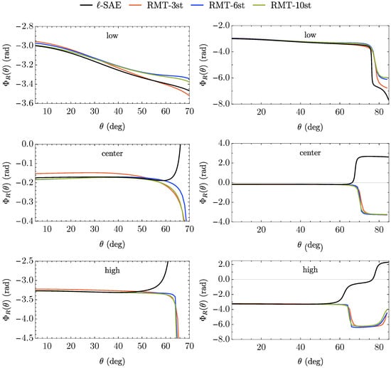
Figure 9.
The RABBITT phase for the SB 14 group (low, center, and high) as a function of the detection angle . Results from the ℓ-SAE approximation and three different RMT models used in [47] are shown. For each SB, the (left panels) show results for , while the (right panels) display the phase for the extended domain .
It is worth noting that running the ℓ-SAE code for a single time delay requires approximately two hours of computing time on a modern personal computer with about 10 cores. In contrast, the same simulation using the 10-state RMT model takes an entire day and nearly 800 processors, thus requiring the use of a supercomputer.
5. Conclusions
In this work, we developed and described the ℓ-SAE approach, which incorporates model potentials that depend on the angular momentum of the active electron. As demonstrated with the helium target, these potentials yield more accurate bound-state energies than those obtainable with the standard SAE approach. The ℓ-SAE method also improves the accuracy of the calculated oscillator strengths, the static and dynamic polarizabilities, and the photoionization cross section.
In the context of TDSE simulations, the inclusion of ℓ-dependent potentials does not require significant modifications to existing SAE computer codes, and the computational resources needed for its implementation remain largely unchanged. As a result, we were able to simulate HHG and 3SB-RABBITT processes efficiently and found that, for the observables of interest here, i.e., single-electron processes, the ℓ-SAE results are of similar accuracy to those from coupled-state all-electron models such as RMT, except for the RABBITT phase for large detection angles.
Finally, we note that the ℓ-SAE approximation can also be extended to study molecular systems, as demonstrated for the diatomic molecule CO2 in [49].
6. A Few Words on Barry Irwin Schneider by J.C.d.V.
I had the chance to talk to Barry a few times, and I was always impressed by his extensive knowledge. In particular, we discussed the LMM, one of the methods used in this work. During our conversations, he encouraged me to develop a user-friendly computational implementation of LMM. Although the idea had already been in my mind for some time, it was Barry’s suggestion that ultimately convinced me to develop such a code. Today, my user-friendly implementation is not only used by myself but also by colleagues and educators, thus furthering the impact of the method.
Author Contributions
J.C.d.V.: methodology, software, validation, formal analysis, and original draft preparation. K.B.: conceptualization, funding acquisition, review and editing. All authors have read and agreed to the published version of the manuscript.
Funding
The authors acknowledge funding from the NSF under grant Nos. PHY-2110023 and PHY-2408484.
Data Availability Statement
The computer codes and data sets generated during the current are available from the corresponding author upon reasonable request.
Acknowledgments
J.C.d.V. is grateful to Drake University for its hospitality, where all calculations for this study were performed. He also thanks the organizers of the Workshop Modern Methods for Differential Equations of Quantum Mechanics 2024 for the invitation to present early results of this work.
Conflicts of Interest
The authors declare no conflicts of interest.
Abbreviations
The following abbreviations are used in this manuscript:
| SAE | Single Active Electron |
| RABBITT | Reconstruction of Attosecond Beating By Interference of Two-photon Transitions |
| TISE | Time-Independent Schrödinger Equation |
| TDSE | Time-Dependent Schrödinger Equation |
| HHG | High-order Harmonic Generation |
| RMT | R-Matrix with Time dependence |
| SB | Side-Band |
| IR | Infra-Red |
| XUV | Extreme Ultra-Violet |
Notes
| 1 | While SAE considerations for molecules are possible, we focus on atomic targets in this work. |
| 2 | As shown in [14], local potentials with ℓ-dependence can be derived from an ℓ-independent non-local potential. |
| 3 | As usual, , and |
| 4 | For example, releasing for . |
| 5 | A factor of 2 is needed in (6) if either or . |
| 6 | A detailed derivation of these equations is provided on pp. 241–244 in [23]. |
References
- Smyth, E.S.; Parker, J.S.; Taylor, K. Numerical Integration of the Time-Dependent Schrödinger Equation for Laser-Driven Helium. Comput. Phys. Commun. 1998, 114, 1–14. [Google Scholar] [CrossRef]
- Brown, A.C.; Armstrong, G.S.; Benda, J.; Clarke, D.D.; Wragg, J.; Hamilton, K.R.; Mašín, Z.; Gorfinkiel, J.D.; van der Hart, H.W. RMT: R-Matrix with Time-Dependence. Solving the Semi-Relativistic, Time-Dependent Schrödinger Equation for General, Multielectron Atoms and Molecules in Intense, Ultrashort, Arbitrarily Polarized Laser Pulses. Comp. Phys. Commun. 2020, 250, 107062. [Google Scholar] [CrossRef]
- Koch, O.; Kreuzer, W.; Scrinzi, A. Approximation of the Time-Dependent Electronic Schrödinger Equation by MCTDHF. Appl. Math. Comput. 2006, 173, 960–976. [Google Scholar] [CrossRef]
- Marques, M.A.; Castro, A.; Bertsch, G.F.; Rubio, A. Octopus: A First-Principles Tool for Excited Electron–Ion Dynamics. Comput. Phys. Commun. 2003, 151, 60–78. [Google Scholar] [CrossRef]
- Bauer, D.; Koval, P. Qprop: A Schrödinger-Solver for Intense Laser–Atom Interaction. Comput. Phys. Commun. 2006, 174, 396–421. [Google Scholar] [CrossRef]
- Fu, Y.; Zeng, J.; Yuan, J. PCTDSE: A Parallel Cartesian-Grid-Based TDSE Solver for Modeling Laser–Atom Interactions. Comput. Phys. Commun. 2017, 210, 181–192. [Google Scholar] [CrossRef]
- Reiff, R.; Joyce, T.; Jaroń-Becker, A.; Becker, A. Single-Active Electron Calculations of High-Order Harmonic Generation from Valence Shells in Atoms for Quantitative Comparison with TDDFT Calculations. J. Phys. Commun. 2020, 4, 065011. [Google Scholar] [CrossRef]
- Cowan, R.D. The Theory of Atomic Structure and Spectra; Los Alamos Series in Basic and Applied Sciences; University of California Press, Ltd.: Berkeley, CA, USA, 1981. [Google Scholar] [CrossRef]
- Kulander, K.; Rescigno, T. Effective Potentials for Time-Dependent Calculations of Multiphoton Processes in Atoms. Comput. Phys. Commun 1991, 63, 523–528. [Google Scholar] [CrossRef]
- Ivanov, I.A.; Kheifets, A.S. Harmonic Generation for Atoms in Fields of Varying Ellipticity: Single-Active-Electron model with Hartree-Fock Potential. Phys. Rev. A 2009, 79, 053827. [Google Scholar] [CrossRef]
- Muller, H.G. Numerical Simulation of High-Order Above-Threshold-Ionization Enhancement in Argon. Phys. Rev. A 1999, 60, 1341–1350. [Google Scholar] [CrossRef]
- Bartschat, K. (Ed.) Computational Atomic Physics: Electron and Positron Collisions with Atoms and Lons; Springer: Berlin/Heidelberg, Germany, 1996. [Google Scholar] [CrossRef]
- Parker, J.S.; Smyth, E.S.; Taylor, K.T. Intense-Field Multiphoton Ionization of Helium. J. Phys. B 1998, 31, L571. [Google Scholar] [CrossRef]
- Lassaut, M.; Vinh Mau, N. l-Dependent Local Potentials Equivalent to a Non-Local Potential. Nucl. Phys. A 1990, 518, 441–448. [Google Scholar] [CrossRef]
- Norcross, D.W. Application of Scattering Theory to the Calculation of Alkali Negative-Ion Bound States. Phys. Rev. Lett. 1974, 32, 192–195. [Google Scholar] [CrossRef]
- Greene, C.H.; Aymar, M. Spin-Orbit Effects in the Heavy Alkaline-Earth Atoms. Phys. Rev. A 1991, 44, 1773–1790. [Google Scholar] [CrossRef]
- Laughlin, C.; Victor, G.A. Model-Potential Methods. In Advances in Atomic and Molecular Physics; Bates, D., Bederson, B., Eds.; Academic Press: Cambridge, MA, USA, 1989; Volume 25, pp. 163–194. [Google Scholar] [CrossRef]
- Marinescu, M.; Sadeghpour, H.R.; Dalgarno, A. Dispersion Coefficients for Alkali-Metal Dimers. Phys. Rev. A 1994, 49, 982–988. [Google Scholar] [CrossRef]
- Moores, D.L.; Norcross, D.W. The Scattering of Electrons by Sodium Atoms. J. Phys. B 1972, 5, 1482. [Google Scholar] [CrossRef]
- Thumm, U.; Norcross, D.W. Evidence for Very Narrow Shape Resonances in Low-Energy Electron-Cs Scattering. Phys. Rev. Lett. 1991, 67, 3495–3498. [Google Scholar] [CrossRef]
- Bartschat, K. Low-Energy Electron Scattering from Caesium Atoms-Comparison of a Semirelativistic Breit-Pauli and a Full Relativistic Dirac Treatment. J. Phys. B 1993, 26, 3595. [Google Scholar] [CrossRef]
- Bray, I. Convergent Close-Coupling Method for the Calculation of Electron Scattering on Hydrogenlike Targets. Phys. Rev. A 1994, 49, 1066–1082. [Google Scholar] [CrossRef]
- Joachain, C.J.; Kylstra, N.J.; Potvliege, R.M. Atoms in Intense Laser Fields; Cambridge University Press: Cambridge, UK, 2011. [Google Scholar] [CrossRef]
- Li, P.C.; Sheu, Y.L.; Laughlin, C.; Chu, S.I. Dynamical Origin of Near- and Below-Threshold Harmonic Generation of Cs in an Intense Mid-Infrared Laser Field. Nat. Commun. 2015, 6, 7178. [Google Scholar] [CrossRef]
- Nikolopoulos, L.A.A. Elements of Photoionization Quantum Dynamics Methods; Morgan & Claypool Publishers: San Rafael, CA, USA, 2019; pp. 2053–2571. [Google Scholar] [CrossRef]
- Perry, M.D.; Szoke, A.; Kulander, K.C. Resonantly Enhanced Above-Threshold Ionization of Helium. Phys. Rev. Lett. 1989, 63, 1058–1061. [Google Scholar] [CrossRef] [PubMed]
- Tong, X.M.; Lin, C.D. Empirical Formula for Static Field Ionization Rates of Atoms and Molecules by Lasers in the Barrier-Suppression Regime. J. Phys. B 2005, 38, 2593. [Google Scholar] [CrossRef]
- Green, A.E.S.; Sellin, D.L.; Zachor, A.S. Analytic Independent-Particle Model for Atoms. Phys. Rev. 1969, 184, 1–9. [Google Scholar] [CrossRef]
- Sarsa, A.; Gálvez, F.; Buendía, E. Parameterized Optimized Effective Potential for the Ground State of the Atoms He through Xe. At. Data Nucl. Data Tables 2004, 88, 163–202. [Google Scholar] [CrossRef]
- Kulander, K.C. Time-Dependent Hartree-Fock Theory of Multiphoton Ionization: Helium. Phys. Rev. A 1987, 36, 2726–2738. [Google Scholar] [CrossRef]
- Kramida, A.; Ralchenko, Y.; Reader, J.; NIST ASD Team. NIST Atomic Spectra Database (Ver. 5.12); National Institute of Standards and Technology: Gaithersburg, MD, USA, 2024. Available online: https://physics.nist.gov/asd (accessed on 25 August 2024). [CrossRef]
- Baye, D. The Lagrange-Mesh Method. Phys. Rep. 2015, 565, 1–107. [Google Scholar] [CrossRef]
- del Valle, J.C.; Nader, D.J. Toward the Theory of the Yukawa Potential. J. Math. Phys. 2018, 59, 102103. [Google Scholar] [CrossRef]
- James, F.; Roos, M. Minuit—A System for Function Minimization and Analysis of the Parameter Errors and Correlations. Comput. Phys. Commun. 1975, 10, 343–367. [Google Scholar] [CrossRef]
- Froese-Fischer, C.; Brage, T.; Jönsson, P. Computational Atomic Structure: An MCHF Approach; Routledge: New York, NY, USA, 1997. [Google Scholar] [CrossRef]
- Birk, P.; Stooß, V.; Hartmann, M.; Borisova, G.D.; Blättermann, A.; Heldt, T.; Bartschat, K.; Ott, C.; Pfeifer, T. Attosecond transient absorption of a continuum threshold. J. Phys. B 2020, 53, 124002. [Google Scholar] [CrossRef]
- Bethe, H.A.; Salpeter, E.E. Quantum Mechanics of One-and Two-Electron Atoms; Springer Science & Business Media: Berlin/Heidelberg, Germany, 2013. [Google Scholar] [CrossRef]
- Drake, G.W.F. (Ed.) Springer Handbook of Atomic, Molecular, and Optical Physics, 2nd ed.; Springer: Berlin/Heidelberg, Germany, 2023. [Google Scholar] [CrossRef]
- Masili, M.; Starace, A.F. Static and Dynamic Dipole Polarizability of the Helium Atom Using Wave Functions Involving Logarithmic Terms. Phys. Rev. A 2003, 68, 012508. [Google Scholar] [CrossRef]
- Starace, A. Photoionization of Atoms. In Springer Handbook of Atomic, Molecular, and Optical Physics; Drake, G.W.F., Ed.; Springer: New York, NY, USA, 2006; pp. 379–390. [Google Scholar] [CrossRef]
- Marr, G.; West, J. Absolute Photoionization Cross-Section Tables for Helium, Neon, Argon, and Krypton in the VUV Spectral Regions. At. Data Nucl. Data Tables 1976, 18, 497–508. [Google Scholar] [CrossRef]
- Douguet, N.; Grum-Grzhimailo, A.N.; Gryzlova, E.V.; Staroselskaya, E.I.; Venzke, J.; Bartschat, K. Photoelectron Angular Distributions in Bichromatic Atomic Ionization Induced by Circularly Polarized VUV Femtosecond Pulses. Phys. Rev. A 2016, 93, 033402. [Google Scholar] [CrossRef]
- Douguet, N.; Bartschat, K. Photoelectron Momentum Distributions in the Strong-Field Ionization of Atomic Hydrogen by Few-Cycle Elliptically Polarized Optical Pulses. Phys. Rev. A 2022, 106, 053112. [Google Scholar] [CrossRef]
- Bondy, A.T.; Saha, S.; del Valle, J.C.; Harth, A.; Douguet, N.; Hamilton, K.R.; Bartschat, K. High-Order Harmonic Generation in Helium: A Comparison Study. Phys. Rev. A 2024, 109, 043113. [Google Scholar] [CrossRef]
- Landau, L.D.; Lifschits, E.M. The Classical Theory of Fields; Course of Theoretical Physics; Pergamon Press: Oxford, UK, 1975; Volume 2. [Google Scholar] [CrossRef]
- Bharti, D.; Srinivas, H.; Shobeiry, F.; Bondy, A.T.; Saha, S.; Hamilton, K.R.; Moshammer, R.; Pfeifer, T.; Bartschat, K.; Harth, A. Multi-sideband Interference Structures by High-Order Photon-Induced Continuum-Continuum Transitions in Helium. Phys. Rev. A 2024, 109, 023110. [Google Scholar] [CrossRef]
- Bondy, A.T.; del Valle, J.C.; Saha, S.; Hamilton, K.R.; Bharti, D.; Harth, A.; Bartschat, K. R-Matrix with Time-Dependence Calculations for Three-Sideband RABBITT in Helium. Eur. Phys. J. D 2024, 78, 106. [Google Scholar] [CrossRef]
- Bharti, D.; del Valle, J.C.; Bondy, A.; Bartschat, K.; Moshammer, R.; Pfeifer, T.; Harth, A. Control of Attosecond Photoemission Time Delays by Quantum-State Interference. 2025; in preparation. [Google Scholar]
- Abu-Samha, M.; Madsen, L.B. Theory of Strong-Field Ionization of Aligned CO2. Phys. Rev. A 2009, 80, 023401. [Google Scholar] [CrossRef]


Disclaimer/Publisher’s Note: The statements, opinions and data contained in all publications are solely those of the individual author(s) and contributor(s) and not of MDPI and/or the editor(s). MDPI and/or the editor(s) disclaim responsibility for any injury to people or property resulting from any ideas, methods, instructions or products referred to in the content. |
© 2025 by the authors. Licensee MDPI, Basel, Switzerland. This article is an open access article distributed under the terms and conditions of the Creative Commons Attribution (CC BY) license (https://creativecommons.org/licenses/by/4.0/).