High-Temperature Optical Spectra of Diatomic Molecules: Influence of the Avoided Level Crossing


Abstract
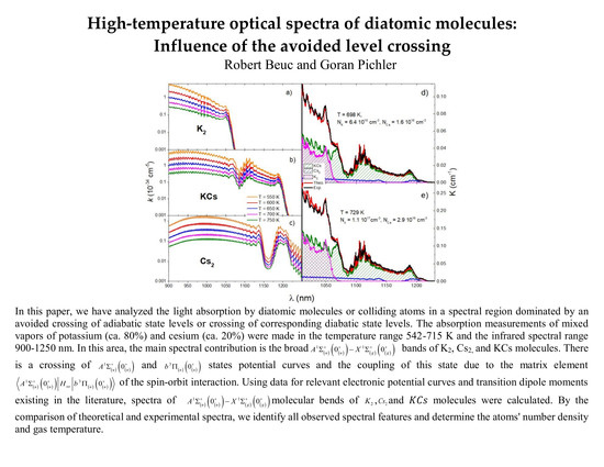
1. Introduction
2. Theoretical Background and Methods
2.1. One Excited Electronic State
2.2. Two Coupled Excited Electronic States
2.3. The Landau–Zener Model
3. Results
3.1. Experiment
3.2. Near-Infrared Spectra of K2, KCs, and Cs2 Molecules
3.3. The Comparison of the Experimental and Theoretical Absorption Coefficient
4. Discussion and Conclusions
Author Contributions
Funding
Conflicts of Interest
References
- Beuc, R.; Movre, M.; Pichler, G. High Temperature Optical Spectra of Diatomic Molecules at Local Thermodynamic Equilibrium. Atoms 2018, 6, 67. [Google Scholar] [CrossRef]
- Девдариани, А.З.; Cебякин Ю., Н. Температурная зависимoсть фoрмы Ландау-Зинерoвскoгo сателита спектральнoй линии. Oпт. и Cпектр. 1976, 48, 1018–1021. [Google Scholar]
- Девдариани, А.З.; Острoвский, В.Н.; Cебякин, Ю.Н. Осoбеннoсти в спектрах электрoнoв и фoтoнoв, свазанные c взаимпдействием квазистациoнарных термoв. ЖЕТФ 1979, 76, 529–542. [Google Scholar]
- Девдариани, А.З.; Cебякин, Ю.Н. Оптическая cпектрoскoпия Ландау-Зинерoвских перехoдoв. ЖЕТФ 1989, 96, 1997–2008. [Google Scholar]
- O’Callaghan, M.J.; Gallagher, A.; Holstein, T. Absorption and emission of radiation in the region of an avoided level crossing. Phys. Rev. A 1985, 32, 2754–2768. [Google Scholar] [CrossRef] [PubMed]
- Landau, L.D. On the theory of energy transmission in collisions I. Phys. Z. Sowjet. 1932, 1, 88. [Google Scholar]
- Zener, C. Non-adiabatic crossing of energy levels. Proc. R. Soc. Lond. A 1932, 137, 696–702. [Google Scholar] [CrossRef]
- Lam, L.K.; Gallagher, A.; Hessel, M.M. The intensity distribution in the Na2 and Li2 A–X bands. J. Chem. Phys. 1977, 66, 3550–3556. [Google Scholar] [CrossRef]
- Chung, H.-K.; Kirby, K.; Babb, J.F. Theoretical study of the absorption spectra of the lithium dimer. Phys. Rev. A 1999, 60, 2002–2008. [Google Scholar] [CrossRef]
- Erdman, P.S.; Larson, C.W.; Fajardo, M.; Sando, K.M.; Stwalley, W.C. Optical absorption of lithium metal vapor at high temperatures. J. Quant. Spectrosc. Radiat. Transf. 2004, 88, 447–481. [Google Scholar] [CrossRef]
- Beuc, R.; Peach, G.; Movre, M.; Horvatić, B. Lithium, sodium and potassium resonance lines pressure broadened by helium atoms. Astron. Astrophys. Trans. 2018, 30, 315–322. [Google Scholar]
- Chung, H.-K.; Kirby, K.; Babb, J.F. Theoretical study of the absorption spectra of the sodium dimer. Phys. Rev. A 2001, 63, 1–8. [Google Scholar] [CrossRef]
- Vadla, C.; Beuc, R.; Horvatic, V.; Movre, M.; Quentmeier, A.; Niemax, K. Comparison of theoretical and experimental red and near infrared absorption spectra in overheated potassium vapor. Eur. Phys. J. D 2006, 37. [Google Scholar] [CrossRef]
- Talbi, F.; Bouledroua, M.; Alioua, K. Theoretical determination of the potassium far-wing photoabsorption spectra. Eur. Phys. J. D 2008, 50, 141–151. [Google Scholar] [CrossRef]
- Beuc, R.; Movre, M.; Horvatić, B. Time-efficient numerical simulation of diatomic molecular spectra. Eur. Phys. J. D 2014, 68. [Google Scholar] [CrossRef]
- Beuc, R.; Movre, M.; Horvatic, V.; Vadla, C.; Dulieu, O.; Aymar, M. Absorption spectroscopy of the rubidium dimer in an overheated vapor: An accurate check of molecular structure and dynamics. Phys. Rev. A 2007, 75. [Google Scholar] [CrossRef]
- Benedict, R.P.; Drummond, D.L.; Schlie, L.A. Fluorescence spectra and kinetics of Cs2. J. Chem. Phys. 1979, 70, 3155. [Google Scholar] [CrossRef]
- Horvatić, B.; Beuc, R.; Movre, M. Numerical simulation of dense cesium vapor emission and absorption spectra. Eur. Phys. J. D 2015, 69, 113. [Google Scholar] [CrossRef]
- Ross, A.J.; Crozeti, P.; Effantint, C.; D’incani, J.; Barrow, R.F. Interactions between the and states of K2. J. Phys. B 1987, 20, 6225–6231. [Google Scholar] [CrossRef]
- Lisdat, C.; Dulieu, O.; Knockel, H.; Tiemann, E. Inversion analysis of K2 coupled electronic states with the Fourier grid method. Eur. Phys. J. D 2001, 17, 319–328. [Google Scholar] [CrossRef]
- Manaa, M.R.; Ross, A.J.; Martin, F.; Crozet, P.; Lyyra, A.M.; Li, L.; Amiot, C.; Bergeman, T. Spin–orbit interactions, new spectral data, and deperturbation of the coupled and states of K2. J. Chem. Phys. 2002, 117, 11208. [Google Scholar] [CrossRef]
- Salami, H.; Bergeman, T.; Beser, B.; Bai, J.; Ahmed, E.H.; Kotochigova, S.A.; Lyyra, M.; Huennekens, J.; Lisdat, C.; Stolyarov, A.V.; et al. Spectroscopic observations, spin-orbit functions, and coupled-channel deperturbation analysis of data on the and of Rb2. Phys. Rev. A 2009, 80, 022515. [Google Scholar] [CrossRef]
- Drozdova, A.N.; Stolyarov, A.V.; Tamanis, M.; Ferber, R.; Crozet, P.; Ross, A.J. Fourier transform spectroscopy and extended deperturbation treatment of the spin-orbit-coupled co and states of the Rb2 molecule. Phys. Rev. A 2013, 88, 022504. [Google Scholar] [CrossRef]
- Verges, J.; Amiot, C. The Cs2 fluorescence excited by the Ar+ 1.09-μm laser line. J. Mol. Spectrosc. 1987, 126, 393–404. [Google Scholar] [CrossRef]
- Bai, J.; Ahmed, E.H.; Beser, B.; Guan, Y.; Kotochigova, S.; Lyyra, A.M.; Ashman, S.; Wolfe, C.M.; Huennekens, J.; Xie, F.; et al. Global analysis of data on the spin-orbit-coupled and states of Cs2. Phys. Rev. A 2011, 83, 032514. [Google Scholar] [CrossRef]
- Kowalczyk, P.; Jastrzebski, W.; Szczepkowski, J.; Pazyuk, E.A.; Stolyarov, A.V. Direct coupled-channels deperturbation analysis of the complex in LiCs with experimental accuracy. J. Chem. Phys. 2015, 142, 234308. [Google Scholar] [CrossRef] [PubMed]
- Grochola, A.; Szczepkowski, J.; Jastrzebski, W.; Kowalczyk, P. Study of the and (0) states in LiCs by a polarization labelling spectroscopy technique. J. Quant. Spectrosc. Radiat. Transf. 2014, 145, 147–152. [Google Scholar] [CrossRef]
- Zaharova, J.; Tamanis, M.; Ferber, R.; Drozdova, A.N.; Pazyuk, E.A.; Stolyarov, A.V. Solution of the fully-mixed-state problem: Direct deperturbation analysis of the complex in a NaCs dimer. Phys. Rev. A 2009, 79, 012508. [Google Scholar] [CrossRef]
- Bergeman, T.; Fellows, C.E.; Gutterres, R.F.; Amiot, C. Analysis of strongly coupled electronic states in diatomic molecules: Low-lying excited states of RbCs. Phys. Rev. A 2003, 67, 050501(R). [Google Scholar] [CrossRef]
- Docenko, O.; Tamanis, M.; Ferber, R.; Bergeman, T.; Kotochigova, S.; Stolyarov, A.V.; Nogueira, A.; Fellows, C.E. Spectroscopic data, spin-orbit functions, and revised analysis of strong perturbative interactions for the and states of RbCs. Phys. Rev. A 2010, 81, 042511. [Google Scholar] [CrossRef]
- Kruzins, A.; Klincare, I.; Nikolayeva, O.; Tamanis, M.; Ferber, R.; Pazyuk, E.A.; Stolyarov, A.V. Fourier-transform spectroscopy of (4) ,, (1)3 transitions in KCs and deperturbation treatment of and . J. Chem. Phys. 2013, 139, 244301. [Google Scholar] [CrossRef] [PubMed]
- Tamanis, M.; Klincare, I.; Kruzins, A.Ž.; Nikolayeva, O.; Ferber, R.; Pazyuk, E.A.; Stolyarov, A.V. Direct excitation of the “dark” state predicted by deperturbation analysis of the complex in KCs. Phys. Rev. A 2010, 82, 032506. [Google Scholar] [CrossRef]
- Borsalino, D.; Vexiau, R.; Aymar, M.; Luc-Koenig, E.; Dulieu, O.; Bouloufa-Maafa, N. Prospects for the formation of ultracold polar ground state KCs molecules via an optical process. J. Phys. B 2016, 49, 055301. [Google Scholar] [CrossRef]
- Janev, R.K. Nonadiabatic Transitions between Ionic and Covalent States. Adv. At. Mol. Phys. 1976. [Google Scholar] [CrossRef]
- Lichten, W. Resonant Charge Exchange in Atomic Collisions. Phys. Rev. 1963, 131, 229. [Google Scholar] [CrossRef]
- Smith, F.T. Diabatic and Adiabatic Representations for Atomic Collision Problems. Phys. Rev. 1969, 179, 111. [Google Scholar] [CrossRef]
- Colbert, D.T.; Miller, W.H. A novel discrete variable representation for quantum mechanical reactive scattering via the S -matrix Kohn method. J. Chem. Phys. 1992, 96, 1982–1991. [Google Scholar] [CrossRef]
- Lam, K.; George, T.F. Semiclassical approach to spontaneous emission of molecular collision systems: A dynamical theory of fluorescence line shapes. J. Chem. Phys. 1982, 76, 3396. [Google Scholar] [CrossRef]
- Beuc, R.; Horvatic, V. The investigation of the satellite rainbow in the spectra of diatomic molecules. J. Phys. B 1992, 25, 1497–1510. [Google Scholar] [CrossRef]
- Kokoouline, V.; Dulieu, O.; Kosloff, R.; Masnou-Seeuws, F. Theoretical treatment of channel mixing in excitedRb2 and Cs2 ultracold molecules: Determination of predissociation lifetimes with coordinate mapping. Phys. Rev. A 2000, 62. [Google Scholar] [CrossRef]
- Beuc, R.; Movre, M.; Mihajlov, A.A. Nonadiabatic affects in absorption line shape. In Proceedings of the 9th International Conference on Spectral Line Shapes, Torun, Poland, 25–29 July 1988; p. D11. [Google Scholar]
- Ovchinnikova, M.Y. Transitions between fine-structure components in resonance interactions for alkali metals. Theor. Exp. Chem. 1965, 1, 12–16. [Google Scholar] [CrossRef]
- Yan, L.; Meyer, W. Electronic state potential curves and electronic transition dipole moments of K2 molecules. Unpublished Results.
- Marinescu, M.; Dalgarno, A. Dispersion forces and long-range electronic transition dipole moments of alkali-metal dimer excited states. Phys. Rev. A 1995, 52, 311. [Google Scholar] [CrossRef] [PubMed]
- Spies, N. Theoretische Untersuchung von Elektronisch Angeregten Zuständen der Moleküle Li2 und Cs2. Ph.D. Thesis, Fachbereich Chemie, Kaiserslautern University, Kaiserslautern, Germany, 1990. [Google Scholar]
- Meyer, W.; Spies, N. Electronic state potential curves of Cs2 molecules. Unpublished Results.
- Allouche, A.R.; Aubert-Frécon, M. Transition dipole moments between the low-lying states of the Rb2 and Cs2 molecules. J. Chem. Phys. 2012, 136, 114302. [Google Scholar] [CrossRef] [PubMed]


| K2 | KCs | Cs2 | |
|---|---|---|---|
| 9.0 | 9.57 | 10.87 | |
| 0.21 | 0.75 | ||
| 0.87 | 0.12 | 0.0056 | |
| 0.13 | 0.88 | 0.9944 |
© 2020 by the authors. Licensee MDPI, Basel, Switzerland. This article is an open access article distributed under the terms and conditions of the Creative Commons Attribution (CC BY) license (http://creativecommons.org/licenses/by/4.0/).
Share and Cite
Beuc, R.; Pichler, G. High-Temperature Optical Spectra of Diatomic Molecules: Influence of the Avoided Level Crossing. Atoms 2020, 8, 28. https://doi.org/10.3390/atoms8020028
Beuc R, Pichler G. High-Temperature Optical Spectra of Diatomic Molecules: Influence of the Avoided Level Crossing. Atoms. 2020; 8(2):28. https://doi.org/10.3390/atoms8020028
Chicago/Turabian StyleBeuc, Robert, and Goran Pichler. 2020. "High-Temperature Optical Spectra of Diatomic Molecules: Influence of the Avoided Level Crossing" Atoms 8, no. 2: 28. https://doi.org/10.3390/atoms8020028
APA StyleBeuc, R., & Pichler, G. (2020). High-Temperature Optical Spectra of Diatomic Molecules: Influence of the Avoided Level Crossing. Atoms, 8(2), 28. https://doi.org/10.3390/atoms8020028