Article

Software Sensors for Order Tracking Applied to Permanent Magnet Synchronous Generator Diagnostics: A Comparative Study

1
Laboratoire d’Informatique et Automatique des Systemes, University of Poitiers, 86073 Poitiers, France
2
LaSIE Laboratory UMR CNRS 7356, University of la Rochelle, 17042 La Rochelle, France
*
Author to whom correspondence should be addressed.
Robotics 2021, 10(2), 59; https://doi.org/10.3390/robotics10020059
Submission received: 9 March 2021 / Revised: 29 March 2021 / Accepted: 4 April 2021 / Published: 8 April 2021

Abstract

:
The paper deals with software sensors which facilitates the diagnosis of electrical machines in non-stationary operating conditions. The technique targeted is order tracking for which different techniques exist to estimate the speed and angle of rotation. However, from a methodological point of view, this paper offers a comparison of several methods in order to evaluate their performance from tests on a test bench. In addition, to perform the tests, it is necessary to initialize the different methods to make them work correctly. In particular, an identification technique is proposed as well as a way to facilitate initialization. The example of this paper is that of a synchronous generator. Angular sampling allows the spectrum to be stationary and the interpretation of a possible defect. The realization of the angular sampling and the first diagnostic elements require the knowledge of two fundamental quantities: the speed of rotation and the angular position of the shaft. The estimation of the rotation speed as well as the estimation of the angular position of the shaft are carried out from the measurement of an electric current (or three electric currents and three voltages). Four methods are proposed and evaluated to realize software sensors: identification technique, PLL (Phase Locked Loop), Concordia transform and an observer. The four methods are evaluated on measurements carried out on a test bench. The results are discussed from the diagnosis of a mechanical fault.

1. Introduction

In many industrial diagnostic applications, operators are faced with cases of non-stationary operating modes. This is, for example, the case in the wind energy sector. In this case, order tracking, carried out from angular sampling, makes it possible to consider the study of the diagnosis of an electromechanical drive in non-stationary operation. For cases where the industrial device does not have a speed sensor or a position sensor, order tracking is really complicated to implement. The major difficulty is the estimation of the speed and the position for the angular resampling. In this context, the main objective of the paper is the order tracking technique from just current measurement. The difficulty is then to estimate the speed of rotation in order to deduce the angle which serves as the synchronization signal for the sampling [1,2]. References [1,2] present a recent and complete bibliography in the case of order tracking, for systems used at variable speed, from a vibratory signal. For this same reference, order tracking from current measurements is not developed in detail. In the case of applications used at a fixed speed, the problem is simpler. One can find interesting results and an important bibliography in reference [3].
The current context, industry 4.0, requires the processing of a large number of data to improve the diagnostic of an industrial installation. The data, for cost reasons, come mainly from software sensors [4]. The signature of faults can be found in different physical quantities: mechanical, acoustic vibrations, temperature, magnetic flux, rotation speed, torque, electric currents, electric voltages, electric powers. More commonly, the diagnosis is in particular possible from the vibration signals [5,6] measured by correctly placed piezoelectric sensors [7] or strain gauges [8]. It is also interesting to be able to make the diagnosis from the measurement of the electric currents which supply a motor. From a physical point of view, many faults are characterized by a harmonic component for which the frequency evolves. In this paper, we consider that the speed is not measured directly. If the speed signal is not available from a sensor, the order tracking is difficult to perform. This additional difficulty requires finding the speed of rotation from a harmonic analysis of the vibratory signal or the “current” signal. As an example, we can give the many electric motors, which in the industry, are not used with a constant rotational speed. The appearance of a fault generally results in the appearance of a harmonic signal which is a multiple of the speed of rotation.
From electrical current signals, to identify a fault, it is possible to search for it in the signal spectrum. An electric current measurement must be processed to extract harmonic components. For the consideration of future use, simplicity is important. This is why software sensors are established from current measurements. The simplest case would be the measurement of a single electric current. This technique is compared to those using the measurement of the three currents. In a non-stationary context, we focus this paper on the extraction of the instantaneous angular speed of rotation and the angular position of the shaft. This information can be used to make an angular sampling of the signals in order to stationarize the signals and therefore the spectrum. The angular sampling part is not developed in this paper. Many papers deal with the frequency estimation of a signal with methods presenting advantages for particular cases. These methods, for an industrial application, present several difficulties: initialization and the possibility of using it in real time [9,10].
The paper [1] presents a survey of techniques used to estimate the rotational speed in the case where no speed sensor is available and in the case where the speed is variable. Many methods are based on vibration measurement. However, it is possible to obtain an estimate of the speed of rotation from the measurement of an electric current (motor power supply) or of the three electric currents (in the case of a three-phase power supply). This paper deals with a comparison of several techniques to help the development of software sensors in order to help the use of order tracking techniques. The context in the research work presented in this paper is that of a diagnostic tool for electrical machines without a speed sensor or angular position sensor. The only measurements used will be the measurements of electric currents (possibly measurements of electrical voltages). The electric machine does not operate at constant speed: case of non-stationary use. In the literature different methods exist, it remains however to specify a methodology for adjusting the parameters. The different methods presented in the paper have already been the subject of previous work, the methods for initializing the parameters are specified and the results obtained are compared. This work allows to consider the choice of a method to develop sensors with angular synchronization for the same benchmark. Thus the calculation of the spectra of the signals x ( θ ) is performed (x can represent for example a current or another physical quantity). This angular synchronization makes it possible to process signals for non-stationary operation.The different techniques presented in this paper can be used either offline or online. The paper also indicates methodological elements and improvement of the initialization phase to help in the choice of a technique compared to another.
The Section 2 details the different methods that are evaluated on a test bench. The tests allow to evaluate the measurement of the speed of rotation of an engine according to the following techniques: technique based on the measurement of a single current (1) or on the measurement of the three currents (three-phase motor) (2) or on the measurement of the three currents and three voltages (3).
For method (1), we first present signal model identification approach (Section 2.1 and secondly a demodulation approach (Section 2.2). For method (2) and method (3), we detail respectively a technique based on the Concordia transform (Section 2.3) and an observer-based technique (Section 2.4).
The paper deals with tools allowing the design of software sensors for monitoring particular frequencies. This approach is a physical approach, the frequencies tracked correspond to physically determined fault frequencies. Other approaches are exploited in this area such as machine learning [11] but they are not discussed in this paper.

2. Frequency Tracking: Different Tools

The different methods exposed can be used from electrical measurements (currents, voltages) to find a harmonic component. The detected frequency is the frequency corresponding to the instantaneous angular speed of rotation.

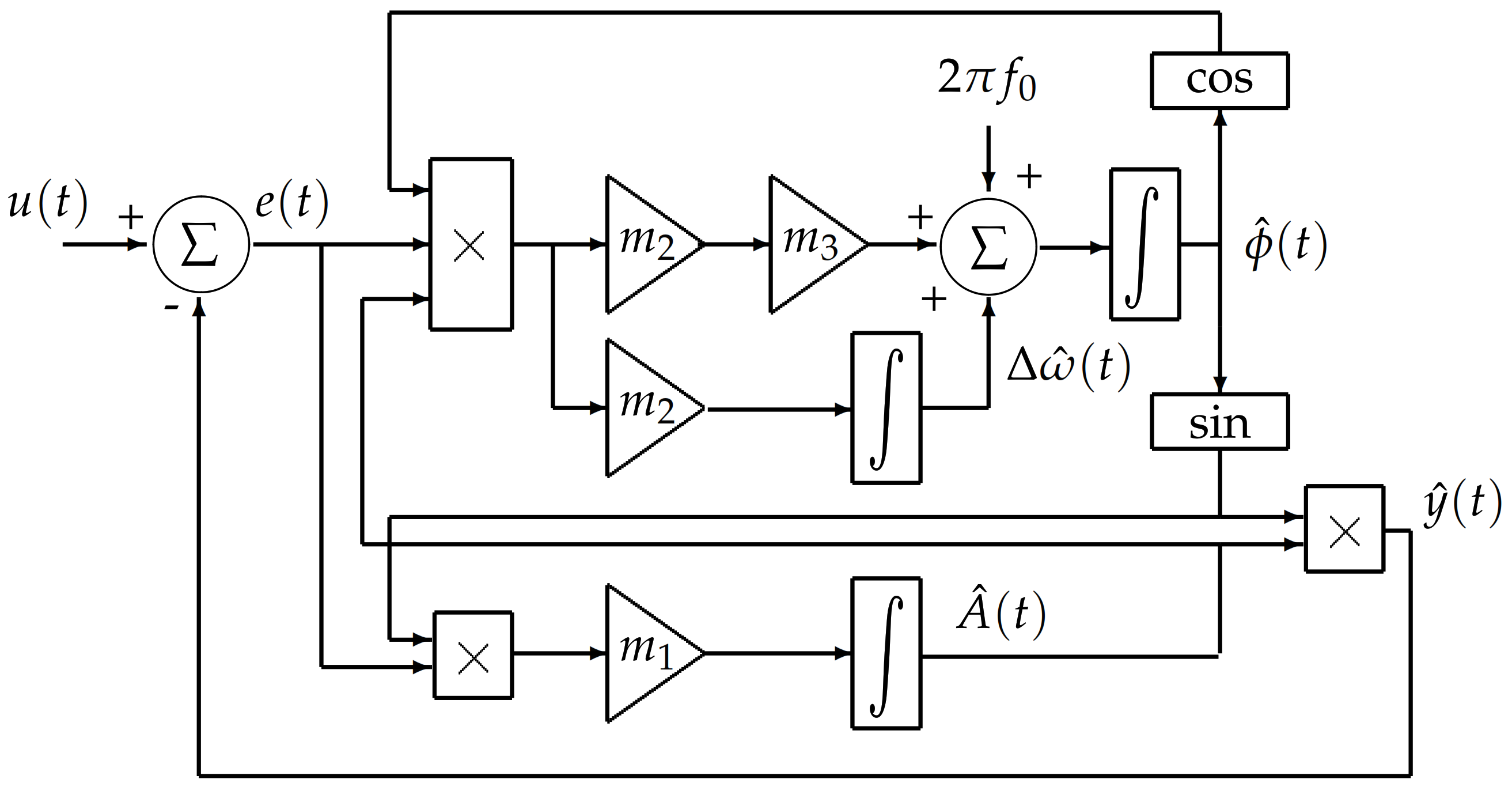
2.1. Signal Model Identification

The algorithm used is a non-linear algorithm based on an adaptive selective filter (notch filter), it was initially proposed in [12] and used in several applications: estimation of symmetrical components in three-phase electrical networks [13], “in situ” efficiency estimation of asynchronous machines [14] and measure harmonics in power electronics [15]. The algorithm is detailed in the article [14] for which Equations (1)–(8) are indicated. This paper takes up the structure proposed in [14] and proposes a new technique for initializing the parameters of the algorithm (detailed below). We recall, that the objective of this paper is to compare the results obtained by this algorithm with three other methods.
Let’s consider a sinusoidal signal:
I f ( t ) = A ( t ) sin φ ( t ) = A ( t ) sin ( ω ( t ) . t + α ( t ) )
To this signal, we add other sinusoidal components and noise n ( t ) :
I ( t ) = i = 0 A i ( t ) sin φ i ( t ) + n ( t )
φ i ( t ) = 0 t w i ( γ ) d γ + α i ( t )
With A ( t ) the signal magnitude, ω ( t ) the pulsation, α ( t ) the phase angle and n ( t ) the noise component. The algorithm uses the gradient method and minimizes the square of the error function:
e ( t ) = I ( t ) A ( t ) sin φ ( t )
The algorithm is based on the following equations:
d A ( t ) d t = m 1 e ( t ) sin φ ( t )
d w ( t ) d t = m 2 e ( t ) A ( t ) cos φ ( t )
d φ ( t ) d t = w ( t ) + m 3 d w ( t ) d t
The functional diagram of the algorithm (Figure 1) shows the use of three parameters, m 1 , m 2 and m 3 . No methodology is specified to initialize the three parameters. The speed of convergence depends on the value of m 1 while m 2 and m 3 have an impact on frequency and phase tracking. We notice the use of integrals in the block diagram, it is therefore very important to correctly initialize the parameters m i to ensure a convergence of the algorithm. This step is developed below.
The Figure 1 shows an interesting algorithm for applications where the instantaneous frequency must be estimated in real time. Indeed, its implementation requires only elements of elementary calculations (additions, subtraction, multiplications, integration).
The identification algorithm allows to estimate both the frequency and the magnitude of a sinusoidal signal. Its realization seems attractive for a “real time” application. However, the initialization of the three parameters m 1 , m 2 and m 3 remains difficult due to the couplings between the magnitude estimation and frequency estimation loops. In addition, the loops are non-linear, which makes setting the parameters a little more complex.
In this paper, we propose to linearize the algorithm presented (Figure 2) in order to help initialize the parameters. Note that linearization degrades the accuracy of the results. However, linearization is the technique we propose to initialize the algorithm. Once the parameters are initialized, the algorithm is used in its initial version. To consider linearization, Figure 2 separates the variations of the signal into two parts: the amplitude part and the frequency part.
The input signal and the output signal are considered respectively as
u ( t ) = ( A 0 + Δ A ( t ) ) s i n ( 2 π ( f 0 + Δ f ( t ) ) t + ϕ 0 )
and
y ( t ) = ( A 0 + Δ A ^ ( t ) ) s i n ( 2 π ( f 0 + Δ f ^ ( t ) ) t + ϕ 0 )
ϕ 0 is the phase of the signals u ( t ) and y ( t ) for t = 0 , it is set to an arbitrary value.
As shown in Figure 2, after linearization, two transfer functions H 1 and H 2 are performed. Linearization results in a decoupling of the estimate of the amplitude and the estimates of the frequency. Thus, the initialization phase, the estimation of the amplitude can be managed independently of the frequency estimation. The calculations are not detailed in this paper. The result of linearization leads to:
H 1 ( s ) = Δ f ^ ( s ) Δ f ( s ) = m 2 A 0 2 π + m 2 m 3 A 0 2 π s s 2 + m 2 m 3 A 0 2 π s + m 2 A 0 2 π
H 2 ( s ) = Δ A ^ ( s ) Δ A ( s ) = 1 1 + s m 1
From the simplified models represented by Equations (10) and (11), resulting from linearization, it is possible to adjust m 1 , m 2 and m 3 to fix the dynamic performance of the estimator algorithm (magnitude and frequency). For example, from the given relation Equation (10), it is necessary to fix a response time ( t r ) as well as a damping coefficient (m) for the system H 1 (model of a 2nd order system). By identification, the value of the parameters m 2 and m 3 can be deduced: m 2 = 9 / ( m 2 A 0 2 π t r 2 ) and m 3 = 2 m 2 t r / 3 .

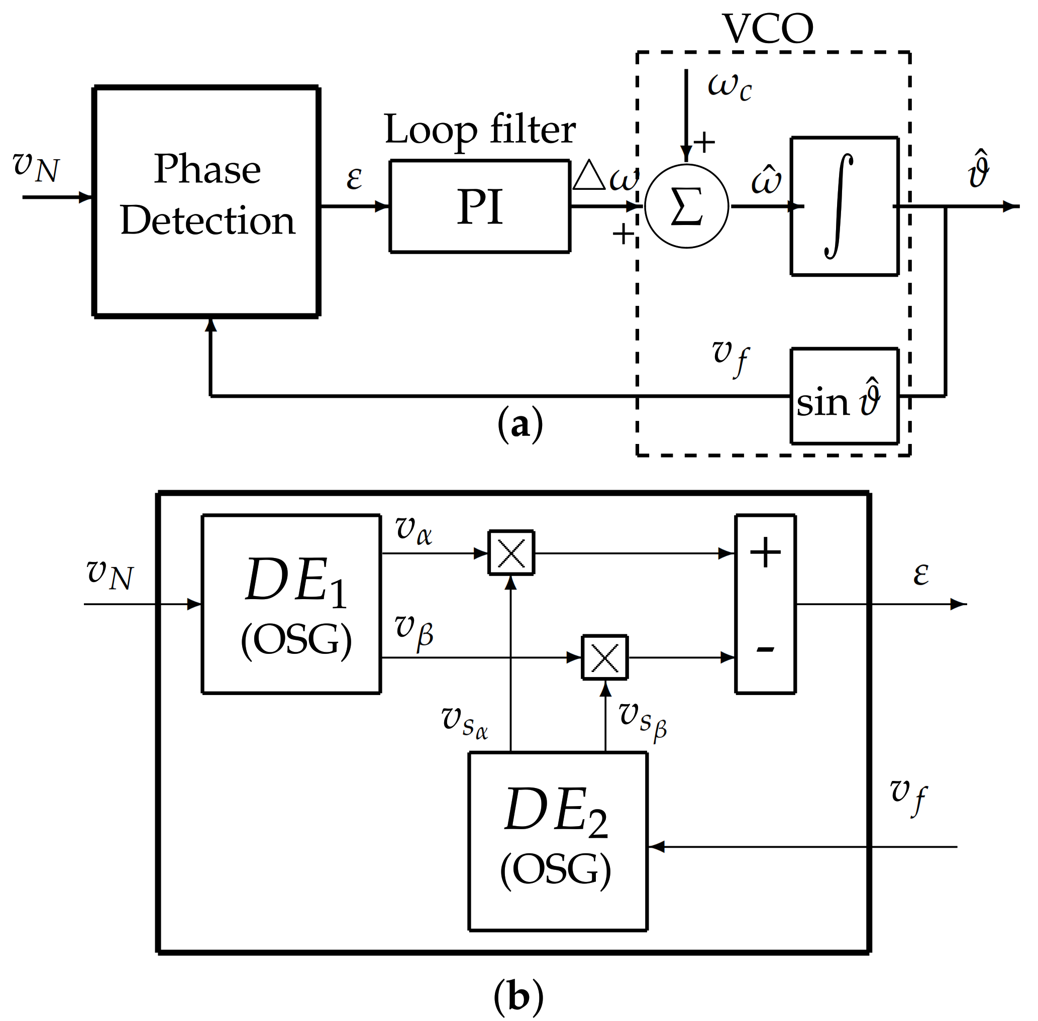
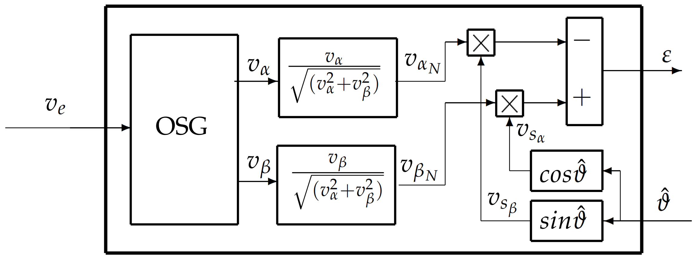
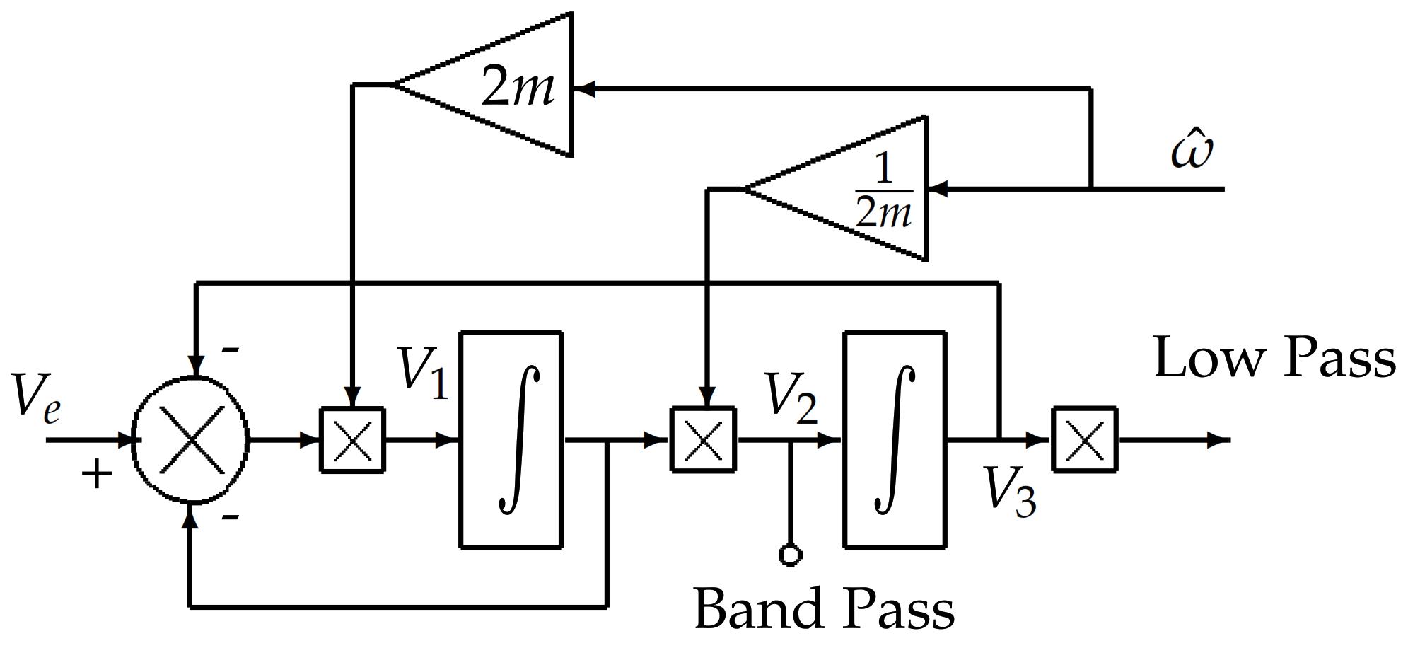
2.2. Demodulation Approach

Phase Locked Loop (PLL) are widely used in different sectors such as communications or electrical networks. The main function sought is the phase or frequency demodulation for which the PLL are efficient in terms of speed and precision, [16]. In general, a PLL is made up of three parts: the phase detector (PD: Phase detector), the loop filter (LF: Loop Filter) and the Voltage Controlled Oscillator (VCO: Voltage controlled oscillator). Many improvements have been made, motivated by the need to design digital PLL [17,18]. The solution most encountered is the use of a Quadrature Phase Detector (QPD) [19]. The QPD uses an orthogonal signal generator (OSG) to create 90-degree phase shifted signals. The harmonic after multiplication is canceled due to orthogonality. The OSG solution appears today as a robust topology against noise and rapid changes.
The OSG proposed by [20] uses two derivative elements (DE: derivative element) to calculate the phase error (Figure 3).
Each block D E x is composed of two filters whose phase difference is constant and equal to π / 2 whatever the frequency of the input signal as shown in the Figure 4.
The transfer functions of the two filters G x and G x are given by:
G x ( s ) = ω R 2 s s 2 + 2 ω R s + ω R 2
G x ( s ) = ω R 2 s 2 + 2 ω R s + ω R 2
with:
-
G x : Bandpass filter with central frequency ω R ,
-
G x : Low-pass with cut-off frequency filter ω R .
More details are given in [21]. This version of the PLL does not work correctly for signals having both a variation of the frequency and a variation of the magnitude. To solve this problem, a normalization of the magnitude of the input signal is proposed.
The structure modified is presented on Figure 5. v α and v β are the output of OSG and are nomalized using the amplitude ( v α 2 + v β 2 ) .
It is noted that, following standardization, the PLL is working properly. If we take the expressions of the two OSG filters (12) and (13), we note these filters are centered on their central pulsation ω R which is fixed here at ω R = 2 π F c . In order to improve the PLL, we use adaptive filters so that the OSG filters can follow the input frequency variations.
The adaptation is carried out according to the estimated pulsation noted ω ^ as indicated in the Figure 6.
In order to realize the adaptive OSG filters, we use a state variable structure (Figure 7).
The adaptation of the input filters associated with normalization now makes it possible to follow the variations in frequency of the input signal while remaining insensitive to variations in magnitude.

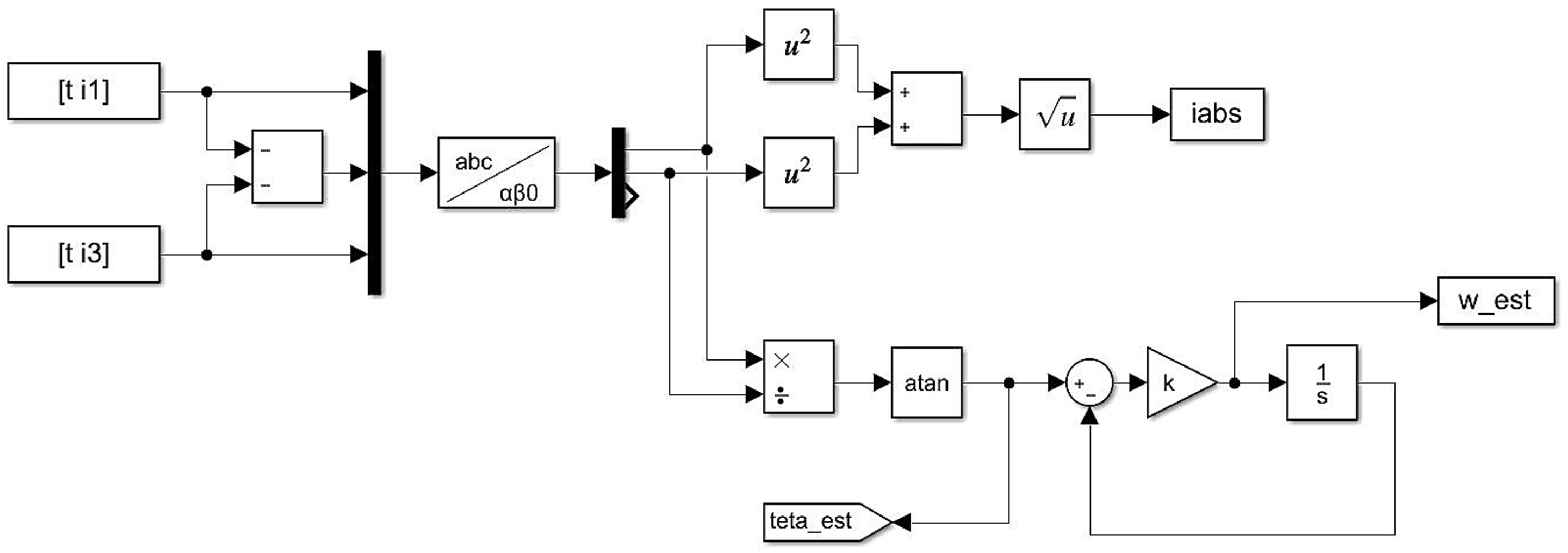
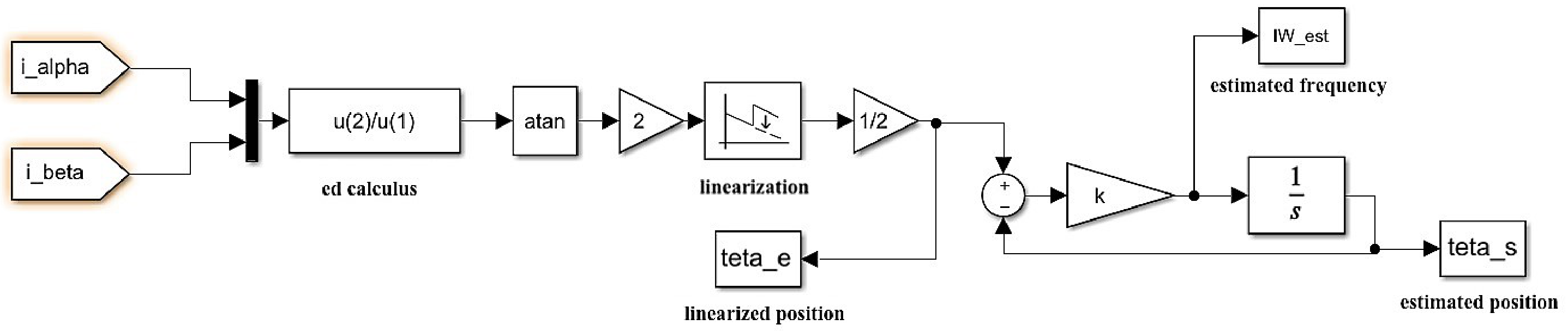
2.3. Concordia Transform Method

When three current measurements are available, the simplest method for estimating the magnitude and the instantaneous phase is the Concordia transform. Consider that the instantaneous magnitude I A ( t ) and the instantaneous frequency I F ( t ) can be estimated by the following relations:
I A ( t ) = i α 2 ( t ) + i β 2 ( t ) ϕ ( t ) = a t a n ( i β ( t ) i α ( t ) ) I F ( t ) = 1 2 π d d t ϕ ( t )
Estimation of different signals can be obtained from two currents under the assumption of load balance (Figure 8).
The instantaneous pulse I W ( t ) is proportional to the derivative of the instantaneous phase I P ( t ) . In practice, we avoid directly calculating this derivative numerically since the current measurements are noisy. An alternative is to use a phase in a closed loop structure (Figure 9).
The system is first order in closed loop. The transfer between the instantaneous phase θ e ( t ) reconstructed by Concordia and the phase estimated at the output of the closed loop θ s ( t ) is a low pass filter.
θ s ( s ) θ e ( s ) = 1 1 + s k
The dynamic is directly fixed by the parameter k. In the case of a phase variation in the ramp (fixed speed for example), There is a speed error.
The transfer between the instantaneous phase θ e ( t ) and the instantaneous pulsation I W e s t ( t ) is a high pass filter.
I W e s t ( s ) θ e ( s ) = s 1 + s k
For k > 1 this transfer is a high pass type (derivative filtered in high frequency) with a constant static gain for the pulsations such as ω > k .
In theory, the transfer between the real instantaneous pulse I W ( t ) and the estimated pulse I W e s t ( t ) at the input of the integrator is governed by the system (15). However, this is only correct if the relation I W ( t ) = d d t I P ( t ) is true. In reality, θ e ( t ) is deduced from the measurement of the currents and from the computation of the function A T A N . The imperfections introduced by these calculation mean that the transfer between I W ( t ) and I W i s ( t ) does not really behave like a first order low pass filter. This will be discussed in the Section 4.
A priori, the transformation of Concordia appears as a solution easy to use to estimate both the mechanical angle and the speed of the electric generator. After a series of tests on the experimental setup, the use of the Concordia transform is tricky. This technique is very sensitive to measurement noise.

2.4. Observer-Based Technique

The adaptive observer used in this subsection is defined as direct and quadrature (d/q) components [22,23]. The rotor speed and the angular position are estimated from the error between the stator currents measured and those estimated by the model. An adaptation mechanism is designed using the error of estimation of the stator currents in order to estimate the speed of the rotor. The adaptive model takes as feedback the output of the adaptation mechanism (i.e., the speed of the rotor). The adaptive observer structure is shown in Figure 10, where the stator currents are chosen as state variables in the adaptive model. Regarding the stability study, the paper specifies the elements that characterize the robustness property of stability from experimental tests.
The adaptive observer model can be written as follows:
ψ ^ ˙ s = u s R s i s ^ p ω ^ m J ψ ^ s + λ i s ˜
with:
-
u s = u d u q T represents the vector of stator voltages.
-
i ^ s = i ^ d i ^ q T represents the vector of stator currents.
-
ψ ^ s = ψ ^ d ψ ^ q T represents the flow stator.
-
R s represents the stator resistance.
-
p ω ^ m = θ ^ ˙ m represents the estimated position of the rotor (rotor angle).
-
J is a square matrix of order 2:
J = 0 1 1 0
-
i s ˜ represents the error of estimation of the stator currents:
i s ˜ = i s i s ^
The flux equation is defined by:
i s ^ = L 1 ψ ^ s ψ p m
with:
-
ψ p m represents the permanent magnet flux expressed as: ψ p m = ψ p m 0 T .
-
L represents the matrix of inductances which depends respectively on the inductances along the direct axis and the quadrature axis L d and L q :
L = L d 0 0 L q
-
λ in the Equation (17) represents the feedback gain matrix. In order to place two poles of the observer in the complex plane at a specific position, λ must include a symmetrical part and an antisymmetric part as follows:
λ = λ 1 I + λ 2 J
with:
-
I represents an identity matrix of order 2.
-
λ 1 and λ 2 represent scalar gains.
The current error is computed as follows:
ϵ = 0 L q · i s ˜
To estimate the electrical angular speed of the rotor, an adaptation based on a proportional-integral regulator (PI) is performed.
ω ^ = p ω ^ m = k p · ϵ k i ϵ · d t
with k p and k i the coefficients of the PI regulator.
The estimated rotor position θ ^ m ( t ) is obtained by integrating the estimated angular speed of the rotor ω ^ m ( t ) .
Usually this type of observer is used for machine control. The observer parameters λ 1 , λ 2 , k p and k i are determined to tune the dynamics of estimation of the currents ( λ 1 , λ 2 ) and the speed ( k p and k i ). In [24], this observer was adjusted specifically for mechanical diagnosis at fixed speed.
For the diagnosis, a study carried out by [24] shows the behavior of the observer and thus makes it possible to adjust parameters λ 1 , λ 2 , k p and k i . By linearization, a study of the dynamic functioning of the observer makes it possible to calculate the transfer functions which allow to compute the speed.
  • F 33 ( s ) = ω ^ ( s ) i d ( s ) .
  • F 34 ( s ) = ω ^ ( s ) i q ( s ) .
  • F 35 ( s ) = ω ^ ( s ) ω ( s ) .
These three transfer functions are shown in the Figure 11.

3. Experimental Setup

The tests are carried out on the test bench presented in this section. However, the tools presented in this paper can be transposed to other synchronous machine technologies. Simply for the observer-based technique, it is necessary to modify the model used.
The test bench is presented on Figure 12. The test machines are synchronous machines from Leroy Somer with their approximate power of 8 kW. They are connected to the electrical network through two speed drivers. The generator operates in regeneration and energy return mode to the electrical network. The speed control strategy or a torque control strategy can be chosen for both machines. They are linked by a COMPABLOC multiplier (LEROY SOMER) with speed ratio N = 4.57 located on the motor side.
A measurement box makes it possible to recover the currents and voltages of the machines. Position measurement is available on low and high speed sides. The measurements are transmitted to a Dspace DS1104 acquisition system with MATLAB/Simulink.
The parameters of each of the machines are found in the Table 1 and Table 2.
The Figure 13 recalls the structure of the software sensor proposed in this paper. The angle measurement, Θ ( t ) is used for angular sampling of the signals. This sampling mode makes it possible to make the spectrum stationary in the case of a non-stationary signal. The Section 4 evaluates the different techniques proposed in this paper by comparing the spectra obtained to a theoretical spectrum.
To evaluate and compare the four proposed techniques, we propose to work on a current signal (or current signals) in the case where there is no fault and in the case where there is a fault. The fault is created from the device described in Figure 14. The device makes it possible to disrupt operation with nine impacts per revolution. The test bench multiplier has a ratio of 4.57 , which therefore corresponds to 1.97 impacts per revolution (generator side). The different algorithms compute hand the speed of rotation and the angle used for an angular sampling of the signal. Therefore, the measured signal no longer depends on time but on the angular position. The signal is denoted x ( Θ ) . With Fourier theory, we calculate the “spectrum” of x ( Θ ) . The result will be expressed in “ev/tr”. Thus, the spectrum is fixed despite the non-stationary operation of the electric machine. The quality of the estimation of the speed and of the angle can be evaluated from the quality of the spectrum. Therefore, on the spectrum obtained with the signal x ( Θ ) , the information to be observed is located at g = g d = 1.97 events per revolution. In fact, the multiplier is defined with a speed ratio N = 4.57 located on the motor side. So with a default of 9 impacts per revolution g = 9 4.57 = 1.97 events per revolution.

4. Experimental Results and Discussion of Numerical Results

From the description of the experimental setup described in Section 3, each technique requires initialization of parameters as indicated in Table 3. The parameters were initialized for each method by considering the dynamics of the magnitude estimation and the frequency estimation. In fact the frequency of rotation evolves over time with a certain dynamic that it is important to consider to initialize the different parameters. The estimation of the rotational speed and the angular position must be made with sufficient dynamics and precision for the angle to be used for angular resampling. The temporal dynamics to extract the value of the angular position must be carried out quickly with respect to the speed of rotation of the machine. So the bandwidth of the software sensor thus developed is greater than the frequency of rotation of the electric machine. Several experimental tests were carried out to initialize the algorithms proposed in this paper.
For Figure 15 and Figure 16, the first plot named “measure” is obtained from the sensors available on the test bench. These plots are used to check and compare the efficiency of the four alogorithms proposed in this paper.
The first results (Figure 15) obtained show the influence of the noise on electric current measurements. In this test, the noisy currents are directly transmitted to the algorithms. Their ability to naturally filter out measurement noise is therefore tested. The recording of 30 cycles has a duration of 3 min and 45 s. First, the algorithms are applied to a faultless data set, then a data set with a default of 9 impacts per revolution on the motor side ( g = g d = 1.97 events per revolution). We define a ratio of the amplitudes found in g = 1.97 events per revolution with and without fault. This ratio is computed by dividing the magnitude of the spectrum defect (with defect) by the average magnitude around the spectrum defect (without defect). For the test considered, the average magnitude is computed in the band [ 1.95 ; 2 ] events per revolution. The results are summarized in the Table 4.
Note that all the methods give estimated noisy speeds, except the PLL. Filters used to normalize the current signal at the PLL input have filtered out noise. When the estimate is too noised, there is a risk that the information about a defect is drowned in the noise. The addition of an additional filter possible, however its adjustment is delicate: it is not necessary to filter the information concerning a sought fault. Despite the noise on the estimated speeds, the identification algorithm and the observer allow the location of the fault by their natural filtering: an integrator (low pass filtering) is necessary to obtain the angular position which is used for the resampling. Note that the least effective method without filtering seems to be the Concordia transform. The Table 4 shows that the ratio calculated for the PLL is the best, which is predictable because this method is the only one which offers bandpass filtering of the signal by its OSG filters.
In this new test, the currents are filtered by a low-pass filter before estimation. The mechanical rotation frequency varies between 2.5 and 12.5 Hz, from an electrical point of view. In fact, for the electric machine we are using, these frequencies correspond to 75 round/min and 375 round/min respectively. The currents are filtered by a first order low-pass filter with a cut-off frequency equal to 100 Hz. The results are given on the Figure 16 and Table 5.
In this test, the estimated speeds are less noisy for all the methods. The speed estimated by Concordia is always noisy, especially at low frequencies. Indeed, in this method, we first estimate the position by the A T A N function and then we derivate to obtain the instantaneous pulsation. Even if the position control allows a derivative filtered at high frequencies, the amplification of the noise remains. The speed estimate has improved for the identification algorithm and for the observer.
To understand the interest of comparing results, it is important to remember the context of the work: tools for the development of a synchronized sensor from an angular position. The signals used are electrical currents and voltages. The electrical machine is used in a non-stationary context. The quality of the estimate with respect to noise is important because the signal obtained by angular synchronization is be used for a future diagnostic step (not treated in this paper). Each method behaves like a filter, the effects of noise are visible on the tests carried out on the test bench.
From the Table 5, by comparing the magnitude ratios, Concordia method seems the weakest to detect the defect compared to the other algorithms. Identification and PLL have a small advantage over the observer. It can be noted that the magnitude of the fault estimated by the observer is the greatest, but the noises are also amplified.

5. Conclusions

In this paper, several methods have been tested allowing to estimate simultaneously the frequency of rotation and the mechanical position of the generator shaft in order to carry out an angular sampling. The comparative tests show good results for the PLL and the monitoring by the observer and Concordia which gives the least good results. This is an interesting result because it is not intuitive. Indeed, on looking here that a single current may be sufficient to achieve the isolation of the component sought. The use of 3 currents does not seem to be a relevant criterion here. The observer also gives good results, but it is necessary to have measurements of tensions and especially the model of the machine that complicates its use in industrial environment. For the two remaining methods, PLL and identification, it seems that the second remains the most robust if we consider the interpretation of the parameters m 1 , m 2 and m 3 as valid.

Author Contributions

L.R., E.E., A.S., T.D. and S.C. proposed the main idea of the paper; A.A., L.R. and E.E. developed differents méthods proposed in this paper. L.R. and T.D. developed the online re-sampling system. A.A. and S.C. implemented simulation verification, analyses and experimental tests. The paper was written by L.R., A.A. and E.E., and was revised by S.C., A.S. and T.D. All the authors were involved in preparing the final version of this manuscript. Besides, this whole work is supervised by L.R., A.A. and E.E. All authors have read and agreed to the published version of the manuscript.

Funding

Research reported in this publication was supported by FEDER Program Poitou-Charentes of the European Union under award number PC158.

Conflicts of Interest

The authors declare no conflict of interest.

References

  1. Lu, S.; Yan, R.; Liu, Y.; Wang, Q. Tacholess Speed Estimation in Order Tracking: A Review With Application to Rotating Machine Fault Diagnosis. IEEE Trans. Instrum. Meas. 2019, 68, 2315–2332. [Google Scholar] [CrossRef]
  2. Peeters, C.; Leclere, Q.; Antoni, J.; Lindahl, P.; Donnal, J.; Leeb, S.; Helsen, J. Review and comparison of tacholess instantaneous speed estimation methods on experimental vibration data. Mech. Syst. Signal Process. 2019, 129, 407–436. [Google Scholar] [CrossRef]
  3. Dineva, A.; Mosavi, A.; Gyimesi, M.; Vajda, I.; Nabipour, N.; Rabczuk, T. applied sciencesArticleFault Diagnosis of Rotating Electrical Machines UsingMulti-Label Classification. Appl. Sci. 2019, 9, 5086. [Google Scholar] [CrossRef] [Green Version]
  4. Kabugo, J.C.; Jämsä-Jounela, S.L.; Schiemann, R.; Binder, C. Industry 4.0 based process data analytics platform: A waste-to-energy plant case study. Int. J. Electr. Power Energy Syst. 2020, 115, 105508. [Google Scholar] [CrossRef]
  5. Dlamini, V.; Naidoo, R.; Manyage, M. A non-intrusive method for estimating motor efficiency using vibration signature analysis. Int. J. Electr. Power Energy Syst. 2013, 45, 384–390. [Google Scholar] [CrossRef] [Green Version]
  6. Yamamoto, G.K.; da Costa, C.; da Silva Sousa, J.S. A smart experimental setup for vibration measurement and imbalance fault detection in rotating machinery. Case Stud. Mech. Syst. Signal Process. 2016, 4, 8–18. [Google Scholar] [CrossRef] [Green Version]
  7. Zhang, H.; Zanchetta, P.; Bradley, K.J.; Gerada, C. A Low-Intrusion Load and Efficiency Evaluation Method for In-Service Motors Using Vibration Tests With an Accelerometer. IEEE Trans. Ind. Appl. 2010, 46, 1341–1349. [Google Scholar] [CrossRef]
  8. Ágoston, K. Vibration Detection of the Electrical Motors using Strain Gauges. Procedia Technol. 2016, 22, 767–772. [Google Scholar] [CrossRef] [Green Version]
  9. Jiang, L.; Li, L.; Zhao, G.; Pan, Y. Instantaneous Frequency Estimation of Nonlinear Frequency-Modulated Signals Under Strong Noise Environment. Circuits, Syst. Signal Process. 2016, 35, 3734–3744. [Google Scholar] [CrossRef]
  10. Liang, Y. Adaptive frequency estimation of sinusoidal signals in colored non-Gaussian noises. Circuits Syst. Signal Process. 2020, 19, 517–533. [Google Scholar] [CrossRef]
  11. Gangsar, P.; Tiwari, R. Signal based condition monitoring techniques for fault detection and diagnosis of induction motors: A state-of-the-art review. Mech. Syst. Signal Process. 2020, 144, 106908. [Google Scholar] [CrossRef]
  12. Ziarani, A.; Konrad, A. A method of extraction of nonstationary sinusoids. Signal Process. 2004, 84, 1323–1346. [Google Scholar] [CrossRef]
  13. Naidoo, R.; Pillay, P.; Visser, J.; Bansal, R.; Mbungu, N. An adaptive method of symmetrical component estimation. Electr. Power Syst. Res. 2018, 158, 45–55. [Google Scholar] [CrossRef]
  14. Siraki, A.G.; Gajjar, C.; Khan, M.A.; Barendse, P.; Pillay, P. An Algorithm for Nonintrusive In Situ Efficiency Estimation of Induction Machines Operating With Unbalanced Supply Conditions. IEEE Trans. Ind. Appl. 2012, 48, 1890–1900. [Google Scholar] [CrossRef] [Green Version]
  15. McNamara, D.; Ziarani, A.; Ortmeyer, T. A New Technique of Measurement of Nonstationary Harmonics. IEEE Trans. Power Deliv. 2007, 22, 387–395. [Google Scholar] [CrossRef]
  16. Golestan, S.; Ramezani, M.; Guerrero, J.M.; Monfared, M. dq-Frame Cascaded Delayed Signal Cancellation- Based PLL: Analysis, Design, and Comparison With Moving Average Filter-Based PLL. IEEE Trans. Power Electron. 2015, 30, 1618–1632. [Google Scholar] [CrossRef] [Green Version]
  17. Han, Y.; Luo, M.; Zhao, X.; Guerrero, J.M.; Xu, L. Comparative Performance Evaluation of Orthogonal-Signal-Generators-Based Single-Phase PLL Algorithms—A Survey. IEEE Trans. Power Electron. 2016, 31, 3932–3944. [Google Scholar] [CrossRef] [Green Version]
  18. Yu, B. An Improved Frequency Measurement Method from the Digital PLL Structure for Single-Phase Grid-Connected PV Applications. Electronics 2018, 7, 150. [Google Scholar] [CrossRef] [Green Version]
  19. Thacker, T.; Boroyevich, D.; Burgos, R.; Wang, F. Phase-Locked Loop Noise Reduction via Phase Detector Implementation for Single-Phase Systems. IEEE Trans. Ind. Electron. 2011, 58, 2482–2490. [Google Scholar] [CrossRef]
  20. Guan, Q.; Zhang, Y.; Kang, Y.; Guerrero, J.M. Single-Phase Phase-Locked Loop Based on Derivative Elements. IEEE Trans. Power Electron. 2017, 32, 4411–4420. [Google Scholar] [CrossRef]
  21. Doget, T.; Etien, E.; Rambault, L.; Cauet, S. A PLL-Based Online Estimation of Induction Motor Consumption Without Electrical Measurement. Electronics 2019, 8, 469. [Google Scholar] [CrossRef] [Green Version]
  22. Omrane, I.; Etien, E.; Dib, W.; Bachelier, O. Modeling and simulation of soft sensor design for real-time speed and position estimation of PMSM. ISA Trans. 2015, 57, 329–339. [Google Scholar] [CrossRef]
  23. Etien, E.; Rambault, L.; Cauet, S.; Sakout, A. Soft sensor design for mechanical fault detection in PMSM at variable speed. Measurement 2016, 94, 326–332. [Google Scholar] [CrossRef]
  24. Masmoudi, M.L. Détection d’un Défaut Localisé dans un Multiplicateur D’éolienne: Approche par Analyse des Grandeurs Électromécaniques. Ph.D. Thesis, University of La Rochelle, La Rochelle, France, 2015. [Google Scholar]
Figure 1. Block diagram of the non-linear identification algorithm, (Diagram from the article by [14]).
Robotics 10 00059 g001
Figure 2. Linearization of the algorithm.
Robotics 10 00059 g002
Figure 3. PLL. (a) Basic structure. (b) Phase detection.
Robotics 10 00059 g003
Figure 4. Bode plot of G x and G x .
Robotics 10 00059 g004
Figure 5. Normalization of PLL entry.
Robotics 10 00059 g005
Figure 6. The PLL input normalization.
Robotics 10 00059 g006
Figure 7. State variable filter diagram.
Robotics 10 00059 g007
Figure 8. Diagram of the estimation of the position and angular speed via Concordia.
Robotics 10 00059 g008
Figure 9. Phase control.
Robotics 10 00059 g009
Figure 10. Block diagram of the system and the adaptive observer.
Robotics 10 00059 g010
Figure 11. Bode plot for F 33 ( s ) , F 34 ( s ) and F 35 ( s ) with k i = 60 , k p = 0.04 , λ 1 = 15 and λ 2 = 0 .
Robotics 10 00059 g011
Figure 12. Laboratory test bench.
Robotics 10 00059 g012
Figure 13. Software sensor for angular sampling.
Robotics 10 00059 g013
Figure 14. Mechanical fault used with the test bench.
Robotics 10 00059 g014
Figure 15. Comparison of methods over 30 cycles and without low-pass filter. The time curves are expressed in mechanical rotation frequency (Hz).
Robotics 10 00059 g015
Figure 16. Comparison of methods over 30 cycles and with low-pass filter. The time curves are expressed in mechanical rotation frequency (Hz).
Robotics 10 00059 g016
Table 1. Characteristics of the permanent magnet synchronous engine.
Engine Characteristics and Parameters
Nominal power P m 7.8 kW
Nominal voltage V360 V
Nominal current I15.6 A
Nominal speed ω l s 750 rpm
Nominal mechanical torque T m 99 N.m
Frequency f50 Hz
Energy efficiency89%
Stator resistance R s 1 Ω
Inductance of the axis d L d 25.7 mH
Inductance of the axis q L q 25.9 mH
Magnetic flux λ 0.8 Wb
Inertia J t 0.0418 Kg.m 2
Encoder resolution1024 points/revolution
Table 2. Characteristics of the permanent magnet synchronous generator.
Characteristics and Parameters of the Generator
Nominal power P m 8.7 kW
Nominal voltage V360 V
Nominal current I16.2 A
Nominal speed ω h s 3000 rpm
Nominal mechanical torque T m 28 N.m
Frequency f200 Hz
Energy efficiency93%
Stator resistance R s 0.6 Ω
Inductance of the axis d L d 6.58 mH
Inductance of the axis q L q 6.6 mH
Magnetic flux λ 0.8 Wb
Inertia J g 0.00663 Kg.m 2
Encoder resolution2500 points/revolution
Table 3. Parameters for setting the estimation methods.
MethodParametersInitialization
Identification m 1 , m 2 , m 3 m 1 = 200 , m 2 = 1800 , m 3 = 0.0133
PLL K p , K i K p = 61 , K i = 367
ConcordiaPhase control: k, τ k = 100 , τ = 0.003
Observer λ 1 , λ 2 , k p , k i λ 1 = 300 , λ 2 = 0 , k p = 0 , k i = 150
Table 4. Comparison table of methods over 30 cycles without low-pass filter. ev/rev: events/revolution and NV: Normalized Voltage.
MethodFrequency of Fault (ev/rev)Magnitude with Fault (NV)Average Magnitude without Fault (NV)Ratio of Magnitudes (without Unit)
Measures1.9680.1000.001952.68
Identification1.9680.0690.00719.78
PLL1.9680.0480.00316.18
Concordia1.9970.7570.31252.42
Observer1.9650.0970.01795.41
Table 5. Comparison table of methods over 30 cycles with low-pass filters. ev/rev: events/revolution and NV: Normalized Voltage.
MethodFrequency of Fault (ev/rev)Magnitude with Fault (NV)Average Magnitude without Fault (NV)Ratio of Magnitudes (without Unit)
Measures1.9680.1000.001952.68
Identification1.9680.0650.003618.25
PLL1.9680.0480.003016.08
Concordia1.9680.0620.01454.28
Observer1.9680.0980.007413.33
Publisher’s Note: MDPI stays neutral with regard to jurisdictional claims in published maps and institutional affiliations.

