Maxwell Points of Dynamical Control Systems Based on Vertical Rolling Disc—Numerical Solutions

Abstract

We study two nilpotent affine control systems derived from the dynamic and control of a vertical rolling disc that is a simplification of a differential drive wheeled mobile robot. For both systems, their controllable Lie algebras are calculated and optimal control problems are formulated, and their Hamiltonian systems of ODEs are derived using the Pontryagin maximum principle. These optimal control problems completely determine the energetically optimal trajectories between two states. Then, a novel numerical algorithm based on optimisation for finding the Maxwell points is presented and tested on these control systems. The results show that the use of such numerical methods can be beneficial in cases where common analytical approaches fail or are impractical.

1. Introduction

The apparatus of Lie groups is commonly used in the control theory of planar non-holonomics mechanisms, such as kinematic cars, robotic snakes, etc. [1,2,3,4,5,6,7,8]. The control Lie group derives a control Lie algebra as a tangent linear space of the group with operation Lie bracket. The main advantage of the control on Lie groups is that everything derived for one point of the mechanism’s configuration space can be easily generalised for all points of the configuration space thanks to the group properties [9,10,11]. For computational reasons, it is preferred that the corresponding Lie algebra be nilpotent. This property generally does not apply, but the Lie algebra can be approximated, usually by an algorithm called a nilpotent approximation or Bellaïche’s algorithm [12,13].

This paper is motivated by [14], where the authors study the Maxwell points of a kinematics model of vertical rolling disk using numerical optimisation methods. The Maxwell point concept is related to optimal control problems [11,15]. At the initial point, the local solution of optimal control problems is the optimal trajectory (referred to as a geodesic), that goes from the initial point and the corresponding control. Maxwell points are points where the geodesics intersect each other for the first time and the corresponding geodesic segments have equal length. For example, Maxwell points on the Heisenberg group lie on the line (see [16]). This implies that Maxwell points are points where geodesics lose optimality. In optimal control problems, there can be other points at which geodesics lose their optimality, for example, conjugate points (see [11,15]).

The problem of existence and finding Maxwell points is an open problem [11,17]. There are only a few concrete situations where the problem is solvable analytically (e.g., the kinematics of a vertical rolling disc) [16,18]. The main goal of this paper is to design a numerical algorithm to find the Maxwell points of the dynamics of a vertical rolling disc. The rolling disk serves as a case study for the methods under development to be tested on, but it may be applicable to a much larger group of complex nonlinear dynamical systems, real-life robots, or may include considerations or models of imperfections of a real dynamical system, as demonstrated in [19].

Using numerical approaches to solve different nonlinear tasks was proven useful in [20,21]. In Section 2 we describe a vertical rolling disc, including the derivation of differential kinematics and dynamics. In particular, we derive the Lie algebra for the differential kinematics and we indicate the shape of the Lie algebra for the dynamics.

In Section 3 and Section 4 we study two different approximations of the Lie algebra for the dynamics of the disc. Later, in Section 3, we use the Taylor polynomial and in Section 4 we use Bellaïche’s algorithm for the approximation of nonlinear expressions, while both approximations give a nilpotent Lie algebra. For both approximated dynamic systems, the optimal control problem is formulated, where the goal is to get an energetically optimal trajectory between two points of the configuration space. We use the Pontryagin maximum principle to derive the ODEs whose solutions give the optimal trajectories.

In Section 5 we show the description of the numerical algorithm developed for finding the Maxwell points of the system. The input of the algorithm is the set of ODEs given by the Pontryagin maximum principle.

Finally, in Section 6 we test the algorithm on both approximated dynamics systems derived in Section 3 and Section 4.

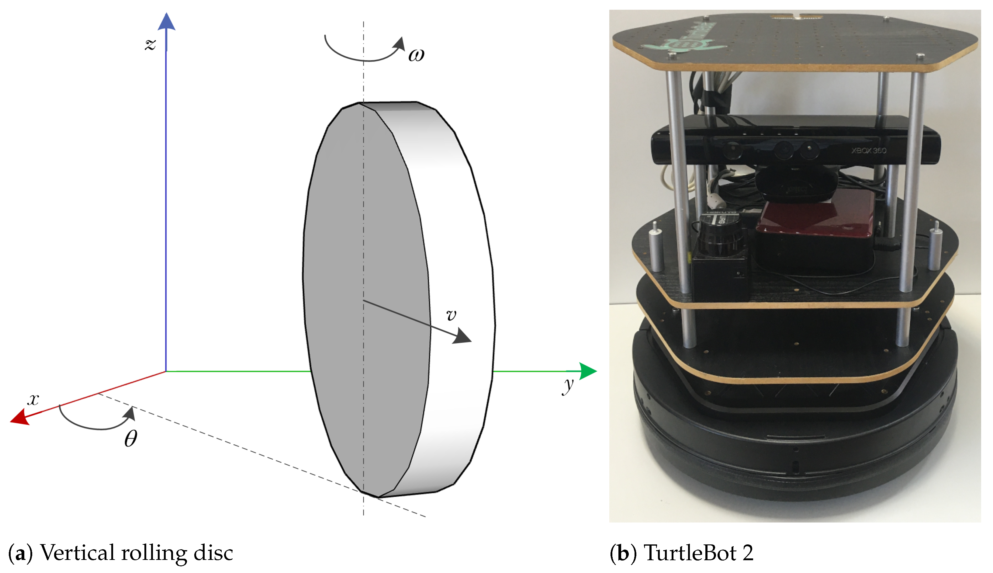
2. Description of the Mechanism

This paper discusses a differential drive wheeled mobile robot’s motion where there are two independent motors and one/two auxiliary wheels (like TurtleBot 2 (Figure 1b), Khepera robot, etc.). Let the mechanism be the homogeneous rolling disc of mass $m=1$ and radius $r=1$ in plane $xy$. Assume that the disc moves without tilting and slipping. It can change the acceleration in the forward or backward direction and the angular acceleration in the vertical axis. The position of the disc can be described by the vector $q={(x,y,\theta ,v,\omega )}^{\mathrm{T}}$, where $\theta$ is its orientation, v its velocity in the forward direction, and $\omega$ the angular velocity (Figure 1a). It gives 5-dimensional configuration space $\mathcal{C}=\{q={(x,y,\theta ,v,\omega )}^{\mathrm{T}}\}$.

2.1. Differential Kinematics of the Mechanism

In this section we want to describe differential kinematics of the mechanism [22,23,24]. The non-slip condition gives us following equation, referred to as the Pfaffian constraint:

$$\begin{array}{c}\hfill (\dot{x},\dot{y})·n=-\dot{x}sin\theta +\dot{y}cos\theta =0.\end{array}$$

(1)

This equation holds if

$$\begin{array}{cc}\hfill \dot{x}& ={\overline{u}}_{1}cos\theta ,\hfill \\ \hfill \dot{y}& ={\overline{u}}_{1}sin\theta ,\hfill \\ \hfill \dot{\theta }& ={\overline{u}}_2,\hfill \end{array}$$

(2)

where ${\overline{u}}_1=v$, ${\overline{u}}_2=\omega$ are control parameters for the kinematics. Note that any movement back and forth can be expressed by $\dot{x}={\overline{u}}_{1}cos\theta ,\dot{y}={\overline{u}}_{1}sin\theta$, and $\dot{\theta }=0$ and any change of the orientation can be expressed as $\dot{x}=0,\dot{y}=0$, and $\dot{\theta }={\overline{u}}_2$. It is obvious that we obtain two vector fields

$$\begin{array}{cc}\hfill {\overline{V}}_1& =cos\theta {\partial }_x+sin\theta {\partial }_y,\hfill \\ \hfill {\overline{V}}_2& ={\partial }_{\theta },\hfill \end{array}$$

(3)

yielding a first-order control system

$$\begin{array}{c}\hfill \dot{\overline{q}}={\overline{u}}_1{\overline{V}}_1+{\overline{u}}_2{\overline{V}}_2,\end{array}$$

(4)

where $\overline{q}={(x,y,\theta )}^{\mathrm{T}}$. The vector fields ${\overline{V}}_1$ and ${\overline{V}}_2$ generate 3-dimensional Lie algebra, where ${\overline{V}}_3=[{\overline{V}}_1,{\overline{V}}_2]=sin\theta {\partial }_x-cos\theta {\partial }_y$. The operation Lie bracket on the algebra is shown in multiplicative

Table 1. Lie bracket of Lie algebra for differential kinematics.

$[·,·]$	${\overline{V}}_1$	${\overline{V}}_2$	${\overline{V}}_3$
${\overline{V}}_1$	0	${\overline{V}}_3$	0
${\overline{V}}_2$	$-{\overline{V}}_3$	0	${\overline{V}}_1$
${\overline{V}}_3$	0	$-{\overline{V}}_1$	0

.

2.2. Dynamics of the Mechanism

The dynamics of the mechanism with respect to movement without tilting and slipping is

$$M\ddot{\overline{q}}=fB-\lambda A,$$

where

$$M=\left(\begin{array}{ccc}m& 0& 0\\ 0& m& 0\\ 0& 0& I\end{array}\right),f=\left(\begin{array}{ccc}F& 0& 0\\ 0& F& 0\\ 0& 0& M_2\end{array}\right),B=\left(\begin{array}{c}cos\theta \\ sin\theta \\ 1\end{array}\right),A=\left(\begin{array}{c}-sin\theta \\ cos\theta \\ 0\end{array}\right),$$

m is the mass of the disk, $I=\frac{1}{4}m{r}^2=\frac{1}{4}$ is the moment of inertia about the vertical axis, r is the radius, F is the force that causes forward and backward movement, $M_2$ is the moment that causes the rotation around the vertical axis, and $\lambda$ is the friction force [25].

For the first derivation of the position the following holds:

$$\dot{\overline{q}}=SV,$$

where

$$S=\left(\begin{array}{cc}cos\theta & 0\\ sin\theta & 0\\ 0& 1\end{array}\right),V=\left(\begin{array}{c}v\\ \omega \end{array}\right),$$

v is the velocity in the direction of the movement and $\omega$ is the angular velocity around the vertical axis. It gives

$$\begin{array}{ccc}\hfill \ddot{\overline{q}}& =& \dot{S}V+S\dot{V},\hfill \\ \hfill S^{\mathrm{T}}M\dot{S}V+S^{\mathrm{T}}MS\dot{V}& =& S^{\mathrm{T}}fB,\hfill \end{array}$$

and it can be derived that

$$\begin{array}{ccc}\hfill \dot{x}& =& vcos\theta ,\hfill \\ \hfill \dot{y}& =& vsin\theta ,\hfill \\ \hfill \dot{\theta }& =& \omega ,\hfill \\ \hfill \dot{v}& =& \frac{F}{m}=\frac{M_1}{mr}=M_1,\hfill \\ \hfill \dot{\omega }& =& \frac{M_2}{I}.\hfill \end{array}$$

(5)

The configuration space is $\mathcal{C}$, $dim\mathcal{C}=5$. The system (5) can be written as

$$\dot{q}=\left(\begin{array}{c}\dot{x}\\ \dot{y}\\ \dot{\theta }\\ \dot{v}\\ \dot{\omega }\end{array}\right)=V_0+u_1{V}_1+u_2{V}_2=\left(\begin{array}{c}vcos\theta \\ vsin\theta \\ \omega \\ 0\\ 0\end{array}\right)+u_1\left(\begin{array}{c}0\\ 0\\ 0\\ 1\\ 0\end{array}\right)+u_2\left(\begin{array}{c}0\\ 0\\ 0\\ 0\\ 4\end{array}\right),$$

(6)

where $u_1=M_1$, $u_2=M_2$ are control parameters for the dynamics. The vector fields $V_0,V_1,V_2$ generate infinitely dimensional Lie algebra, so for a discussion of controllability, the vector fields need to be approximated appropriately.

3. Approximation of Vector Fields Using Taylor Polynomial

An approximation by the Taylor polynomial is offered as one of the possibilities. Using a Taylor polynomial of the first order at point $\theta =0$ we get $cos\theta \approx 1$, $sin\theta \approx \theta$. Then the dynamics of the mechanism is

$$\dot{q}=\left(\begin{array}{c}\dot{x}\\ \dot{y}\\ \dot{\theta }\\ \dot{v}\\ \dot{\omega }\end{array}\right)={\tilde{V}}_0+u_1{\tilde{V}}_1+u_2{\tilde{V}}_2=\left(\begin{array}{c}v\\ v\theta \\ \omega \\ 0\\ 0\end{array}\right)+u_1\left(\begin{array}{c}0\\ 0\\ 0\\ 1\\ 0\end{array}\right)+u_2\left(\begin{array}{c}0\\ 0\\ 0\\ 0\\ 4\end{array}\right).$$

(7)

The vector fields ${\tilde{V}}_0,{\tilde{V}}_1,{\tilde{V}}_2$ generate 8-dimensional nilpotent Lie algebra, where

$$\begin{array}{ccc}\hfill {\tilde{V}}_3& =& [{\tilde{V}}_0,{\tilde{V}}_1]=-{\partial }_x-\theta {\partial }_y,\hfill \\ \hfill {\tilde{V}}_4& =& [{\tilde{V}}_0,{\tilde{V}}_2]=-4{\partial }_{\theta },\hfill \\ \hfill {\tilde{V}}_5& =& [{\tilde{V}}_0,{\tilde{V}}_3]=-\omega {\partial }_y,\hfill \\ \hfill {\tilde{V}}_6& =& [{\tilde{V}}_0,{\tilde{V}}_4]=4v{\partial }_y,\hfill \\ \hfill {\tilde{V}}_7& =& [{\tilde{V}}_3,{\tilde{V}}_4]=-4{\partial }_y.\hfill \end{array}$$

The operation Lie bracket on the algebra is shown in multiplicative

Table 2. Lie algebra of approximated vector fields using Taylor polynomial.

$[·,·]$	${\tilde{V}}_0$	${\tilde{V}}_1$	${\tilde{V}}_2$	${\tilde{V}}_3$	${\tilde{V}}_4$	${\tilde{V}}_5$	${\tilde{V}}_6$	${\tilde{V}}_7$
${\tilde{V}}_0$	0	${\tilde{V}}_3$	${\tilde{V}}_4$	${\tilde{V}}_5$	${\tilde{V}}_6$	0	0	0
${\tilde{V}}_1$	$-{\tilde{V}}_3$	0	0	0	0	0	$-{\tilde{V}}_7$	0
${\tilde{V}}_2$	$-{\tilde{V}}_4$	0	0	0	0	${\tilde{V}}_7$	0	0
${\tilde{V}}_3$	$-{\tilde{V}}_5$	0	0	0	${\tilde{V}}_7$	0	0	0
${\tilde{V}}_4$	$-{\tilde{V}}_6$	0	0	$-{\tilde{V}}_7$	0	0	0	0
${\tilde{V}}_5$	0	0	$-{\tilde{V}}_7$	0	0	0	0	0
${\tilde{V}}_6$	0	${\tilde{V}}_7$	0	0	0	0	0	0
${\tilde{V}}_7$	0	0	0	0	0	0	0	0

.

We can see that the Lie algebra is nilpotent but the dimension of the algebra is higher than the dimension of the configuration space $\mathcal{C}$. However, at point $q_0={(0,0,0,0,0)}^{\mathrm{T}}$ we get nilpotent sub-algebra of dimension 5, so the mechanism is locally controllable. In Section 4 we compute the approximation of vector fields $V_0,V_1,V_3$ using Bellaïche’s algorithm to get nilpotent algebra of dimension 5.

3.1. Optimal Control Problem

The dynamics (7) with conditions

$$\begin{array}{c}\hfill \begin{array}{cc}\hfill & q\left(0\right)=q_0,q_0={(0,0,0,0,0)}^{\mathrm{T}},\hfill \\ \hfill & q\left(T\right)=q_T,\hfill \end{array}\end{array}$$

(8)

and optimality condition

$$L={\int }_0^T(u_1^2+u_2^2)\mathrm{d}t\to min$$

(9)

gives the optimal control problem whose solution gives an energetically optimal trajectory between two points $q_0,q_T\in \mathcal{C}$, where $u_1,u_2$ are control parameters and T is the end time. The Hamiltonian of the optimal control problem is

$$H=\underset{u_1,u_2\in \mathbb{R}}{max}\left[(u_1^2+u_2^2)h_0+v{h}_1+v\theta h_2+\omega h_3+u_1{h}_4+4u_2{h}_5\right].$$

Using PMP we get the optimality conditions $\frac{\partial H}{\partial u_1}=0,\frac{\partial H}{\partial u_2}=0$. This gives

$$\begin{array}{c}\hfill \begin{array}{cc}\hfill u_1& =-\frac{h_4}{2h_0},\hfill \\ \hfill u_2& =-\frac{2h_5}{h_0},\hfill \end{array}\end{array}$$

(10)

so the Hamiltonian is in the form

$$H=-\frac{h_4^2}{4h_0}-\frac{4h_5^2}{h_0}+v{h}_1+v\theta h_2+\omega h_3.$$

The adjoint system and the dynamics of the mechanism (7) with respect to (10) gives the following system of differential equations:

$$\begin{array}{c}\hfill \begin{array}{cc}\hfill {\dot{h}}_i& =-\frac{\partial H}{\partial x_i},i\in \{0,1,\cdots ,5\},\hfill \\ \hfill \dot{q}& ={\tilde{V}}_0-\frac{h_1}{2h_0}{\tilde{V}}_1-\frac{8h_2}{h_0}{\tilde{V}}_2,\hfill \end{array}\end{array}$$

(11)

where $x_i\in \{x,y,\theta ,v,\omega \}$. The solution of the system with respect to (8) gives the optimal curve between points $q_0,q_T\in \mathcal{C}$. The corresponding control $u_1,u_2$ can be found from (10).

4. Nilpotent Approximation Using Bellaïche’s Algorithm

In this section we would like to find 5-dimensional nilpotent algebra that approximates the algebra generated by vector fields $V_0,V_1,V_2$ derived in (6). Let us introduce some notions. Define ${\Delta }^1$ to be the linear subspace generated by $X_1,\dots ,X_m,$

$${\Delta }^1=\mathrm{span}\{X_1,\cdots ,X_m\}$$

For $s\ge 1,$ define ${\Delta }^{s+1}={\Delta }^s+[{\Delta }^1,{\Delta }^s].$ Set $n_i\left(p\right)=\dim {\Delta }^i\left(p\right).$ We define weights at $p,w_i=w_i\left(p\right),i=1,\cdots ,n$ by setting $w_j=s$ if $n_{s-1}\left(p\right)<j\le n_s\left(p\right),$ where $n_0=0.$

In the construction of a nilpotent approximation of the given Lie algebra we will first proceed with the construction of privileged coordinates according to Bellaïche’s algorithm [12].

• Choose an adapted frame $Y_1,\cdots ,Y_n$ at p.
  In our case we choose frame $(Y_1:=V_0,Y_2:=V_1,Y_3:=V_2,Y_4:=V_3,Y_5:=V_4)$ at $p=(0,0,0,1,0)$.
• Choose coordinates $(y_1,\cdots ,y_n)$ centered at p such that ${\partial }_{y_i}{|}_p=Y_i\left(p\right)$.
  For our adapted frame we choose the coordinates

  $$\left(\begin{array}{c}{y}_1\\ y_2\\ y_3\\ y_4\\ y_5\end{array}\right)=\left(\begin{array}{ccccc}0& 0& 0& 1& 0\\ 0& 0& 0& 0& 4\\ 1& 0& 0& 0& 0\\ 0& 0& 4& 0& 0\\ 0& -4& 0& 0& 0\end{array}\right)\left(\begin{array}{c}x\\ y\\ \theta \\ v\\ \omega \end{array}\right).$$
• For $j=1,\cdots ,n$ set

  $$z_j=y_j-\sum _{k=2}^{w_j-1}{h}_k(y_1,\cdots ,y_{j-1}),$$

  where, for $k=2,\cdots ,w_j-1$

  $$h_k(y_1,\cdots ,y_{j-1})=\sum _{\begin{array}{c}\left|\alpha \right|=k\\ w\left(\alpha \right)<w_j\end{array}}{Y}_1^{{\alpha }_1}\cdots Y_{j-1}^{{\alpha }_{j-1}}\left(y_j-\sum _{q=2}^{k-1}{h}_q\left(y\right)\right)\left(p\right)\frac{y_1^{{\alpha }_1}}{{\alpha }_1}\cdots \frac{y_{j-1}^{{\alpha }_{j-1}}}{{\alpha }_{j-1}},$$

  with $\left|\alpha \right|={\alpha }_1+\cdots +{\alpha }_n.$ First notice that for coordinates of degree $w_i<3$ the transformation $z_i=h(y_1,\cdots ,y_i)$ degenerates [12]. Thus, we will focus on the evaluation of $z_5.$ The sum yields

  $$\begin{array}{cc}\hfill \sum _{k=2}^{w_j-1}{h}_k(y_1,\cdots ,y_{j-1})& =h_2(y_1,\cdots ,y_4)\hfill \\ & =Y_1{Y}_2\left(y_5\right)\left(p\right)y_1{y}_2+Y_1{Y}_3\left(y_5\right)\left(p\right)y_1{y}_3+\hfill \\ & +Y_1{Y}_4\left(y_5\right)\left(p\right)y_1{y}_4+Y_2{Y}_3\left(y_5\right)\left(p\right)y_2{y}_3+\hfill \\ & +Y_3{Y}_4\left(y_5\right)\left(p\right)y_3{y}_4+Y_2{Y}_4\left(y_5\right)\left(p\right)y_2{y}_4+\hfill \\ & +Y_1^2\left(y_5\right)\left(p\right)y_1^2+Y_2^2\left(y_5\right)\left(p\right)y_2^2+Y_3^2\left(y_5\right)\left(p\right)y_3^2.\hfill \end{array}$$

  Notice that $Y_2\left(y_5\right)=0$, $Y_4\left(y_5\right)=0$ and furthermore $Y_1^2\left(y_5\right)=0$, $Y_3^2\left(y_5\right)=0$, $Y_2{Y}_3\left(y_5\right)=0$. So, the transformations $z_i$ are of the form

  $$\begin{array}{cc}\hfill z_1& =y_1,\hfill \\ \hfill z_2& =y_2,\hfill \\ \hfill z_3& =y_3,\hfill \\ \hfill z_4& =y_4,\hfill \\ \hfill z_5& =y_5+\frac{1}{4}sin\left(\frac{y_4}{4}\right)\left(p\right)y_1{y}_3,\hfill \end{array}$$

  in original coordinates $(x,y,\theta ,v,\omega )$

  $$\begin{array}{cc}\hfill z_1& =v,\hfill \\ \hfill z_2& =4\omega ,\hfill \\ \hfill z_3& =x,\hfill \\ \hfill z_4& =4\theta ,\hfill \\ \hfill z_5& =-4y+\frac{1}{4}sin\left(\theta \right)\left(p\right)vx.\hfill \end{array}$$

  We can see that for the choice of $\theta =0$ the transformation degenerates, and hence from now on let us introduce a substitution $C=\frac{1}{4}{sin\left(\theta \right)|}_p.$ Now, express the base of tangent bundle of old coordinates in terms of new coordinates
  $$\begin{array}{cc}\hfill {\partial }_x& ={\partial }_{z_3}+C{z}_1{\partial }_{z_5},\hfill \\ \hfill {\partial }_y& =-4{\partial }_{z_5},\hfill \\ \hfill {\partial }_{\theta }& =4{\partial }_{z_4},\hfill \\ \hfill {\partial }_v& ={\partial }_{z_1}+C{z}_3{\partial }_{z_5},\hfill \\ \hfill {\partial }_{\omega }& =4{\partial }_{z_2}.\hfill \end{array}$$

Finally, let us express original vector fields in algebraic privileged coordinates.

$$\begin{array}{cc}\hfill {\overline{N}}_0& =z_1{\partial }_{z_3}+C{z}_1^2{\partial }_{z_5}-z_1{z}_4{\partial }_{z_3}+16z_2{\partial }_{z_4},\hfill \\ \hfill {\overline{N}}_1& ={\partial }_{z_1}+C{z}_3{\partial }_{z_5},\hfill \\ \hfill {\overline{N}}_2& =16{\partial }_{z_2},\hfill \\ \hfill {\overline{N}}_3& =16{\partial }_{z_4},\hfill \\ \hfill {\overline{N}}_4& =z_1{z}_4{\partial }_{z_3}+(C{z}_1^2{z}_4+16z_1){\partial }_{z_5}.\hfill \end{array}$$

The second step of nilpotent approximation is the approximation of the vector fields’ elements (from a function viewpoint). First let us define a weighted degree of monomial. Given a sequence of integers $\alpha =({\alpha }_1,\dots ,{\alpha }_n),$ we define the weighted degree of the monomial $z^{\alpha }=z_1^{{\alpha }_1}\dots z_n^{{\alpha }_n}$ to be $w\left(\alpha \right)=w_1{\alpha }_1+\dots +w_n{\alpha }_n$ and the weighted degree of the monomial vector field $z^{\alpha }{\partial }_{z_j}$ to be $w\left(\alpha \right)-w_j.$

For vector field X with a Taylor expansion

$$X\left(z\right)\sim \sum _{\alpha ,j}{a}_{\alpha ,j}{z}^{\alpha }{\partial }_{z_j},$$

the order of X is the least weighted degree of a monomial vector field having a nonzero coefficient in the Taylor series. Grouping together the monomial vector fields of the same weighted degree we can express each vector field as a series of monomial vector fields. A monomial vector field with the least weighted degree gives us nilpotent approximation of the Lie algebra [13], thus

$$\begin{array}{cc}\hfill N_0& ={\partial }_{z_3}-z_4{\partial }_{z_5}+16z_2{\partial }_{z_4},\hfill \\ \hfill N_1& ={\partial }_{z_1},\hfill \\ \hfill N_2& =16{\partial }_{z_2},\hfill \\ \hfill N_3& =16{\partial }_{z_4},\hfill \\ \hfill N_4& =16{\partial }_{z_5}.\hfill \end{array}$$

The operation Lie bracket on the algebra is shown in multiplicative

Table 3. Lie bracket of nilpotent Lie algebra found by Bellaïche’s algorithm.

$[·,·]$	$N_0$	$N_1$	$N_2$	$N_3$	$N_4$
$N_0$	0	0	$-16N_3$	$N_4$	0
$N_1$	0	0	0	0	0
$N_2$	$16N_3$	0	0	0	0
$N_3$	$-N_4$	0	0	0	0
$N_4$	0	0	0	0	0

.

4.1. Optimal Control Problem

The dynamics of the mechanism

$$\dot{q}=\left(\begin{array}{c}{\dot{z}}_1\\ {\dot{z}}_2\\ {\dot{z}}_3\\ {\dot{z}}_4\\ {\dot{z}}_5\end{array}\right)=N_0+u_1{N}_1+u_2{N}_2=\left(\begin{array}{c}0\\ 0\\ 1\\ 16z_2\\ -z_4\end{array}\right)+u_1\left(\begin{array}{c}1\\ 0\\ 0\\ 0\\ 0\end{array}\right)+u_2\left(\begin{array}{c}0\\ 16\\ 0\\ 0\\ 0\end{array}\right),$$

(12)

and conditions (8) and (9) define a different approximation of the same optimal control problem as in Section 3. Like in Section 3 we get that for the control the following hold:

$$\begin{array}{c}\hfill \begin{array}{cc}\hfill u_1& =-\frac{h_1}{2h_0},\hfill \\ \hfill u_2& =-\frac{8h_2}{h_0}.\hfill \end{array}\end{array}$$

(13)

The Hamiltonian is in the form

$$H=-\frac{h_4^2}{4h_0}-\frac{64h_5^2}{h_0}+h_3+16z_2{h}_4-z_4{h}_5,$$

and the system of differential equations is in the form

$$\begin{array}{c}\hfill \begin{array}{cc}\hfill {\dot{h}}_i& =-\frac{\partial H}{\partial z_i},i\in \{0,1,...,5\},\hfill \\ \hfill \dot{q}& =N_0-\frac{h_1}{2h_0}{N}_1-\frac{8h_2}{h_0}{N}_2.\hfill \end{array}\end{array}$$

(14)

The solution of the system with respect to (8) gives the optimal curve between points $q_0,q_T\in \mathcal{C}$.

5. Numerical Analysis

As stated in the previous sections, obtaining the Maxwell points of the system is crucial if our goal is to solve the optimal control problem. However, finding them analytically is not always possible, and even if an analytical solution is technically reachable it may not be a practically feasible one.

In practice, a viable alternative to analytical methods is a numerical solution to the problem. Therefore, we developed a numerical apparatus to help discover the approximate location of these Maxwell points of a dynamical system, and to be able to validate any Maxwell point candidates.

The numerical approach proposed throughout this section utilises the Maxwell point definition in the form: a Maxwell point (MP) is any state of an autonomous dynamical system such that it is the end point of (at least) two different trajectories equal in both length in the state space and time, starting at any given state. Generally, there is no guarantee that Maxwell points exist in any given case. However, when presented with a specific system, we can attempt to find them using this definition, and if the attempt fails it can be presumed that the Maxwell points do not exist.

To describe the methods used in further subsections a basic nomenclature will be described here. First, we assume that we deal with an autonomous system of ODEs—the control system, which was created by expanding the original system using the PMP as described in Section 3.1 and Section 4.1, resulting in the explicit form (15)

$$\dot{\mathit{y}}=\mathit{f}\left(\mathit{q},\mathit{h}\right)=\mathit{f}\left(\mathit{y}\right),$$

(15)

where $\mathit{y}\in {\mathbb{R}}^{2n}$ is the state space of the control system, $\mathit{q}\in {\mathbb{R}}^n$ is the state space of the original system, and $\mathit{h}\in {\mathbb{R}}^n$ is the extended space generated by the PMP with respect to a minimisation functional $L\left(\mathit{y},t\right)$ described by Equation (9).

These spaces are related as

$$\mathit{y}=\left[\begin{array}{c}\mathit{q}\\ \mathit{h}\end{array}\right],\mathit{q}=\left[\begin{array}{c}{q}_1\\ ⋮\\ q_n\end{array}\right],\mathit{h}=\left[\begin{array}{c}{h}_1\\ ⋮\\ h_n\end{array}\right]$$

(16)

Additionally, we denote a specific state at a given time instant as $\mathit{q}\left(t\right)={\mathit{q}}_t$, for example, $\mathit{q}\left(0\right)={\mathit{q}}_0$ representing the initial state or $\mathit{q}\left(T\right)={\mathit{q}}_T$ the final state, if $t\in \left(0;T\right)$. If more than one state trajectory is being described, the respective states are marked ${\mathit{q}}_i\left(t\right)={\mathit{q}}_{it}$, with i being the trajectory index. The same notation is used for vectors y, q, and h.

Given this formulation, the task of looking for a Maxwell point in the q space corresponds to solving the boundary value problem for a system described by (15) with the boundary values given by any ${\mathit{q}}_0$ and ${\mathit{q}}_T={\mathit{q}}_M$ representing the Maxwell point. Note that we only trace the position of Maxwell points in the state space of the original system q, not in the whole state space of the control system y.

Further, given an initial condition ${\mathit{y}}_0=[{\mathit{q}}_0^{\mathrm{T}},{\mathit{h}}_0^{\mathrm{T}}]={[q_{10}\dots h_{n0}]}^{\mathrm{T}}$ we can simulate the system numerically and produce a trajectory using numerical integration methods such as Runge–Kutta [26]. This allows us to acquire trajectory end points. Different system trajectories can be generated using different initial conditions. These properties allow us to effectively convert the BVP solution, which is generally a very difficult task, to an IVP coupled with an optimisation algorithm (commonly referred to as the shooting method) [27].

As stated earlier, if a point is a Maxwell point of the system, then two different trajectories from the same initial point ${\mathit{q}}_0$ will intersect at time T at this point. Based on this assumption we can now reformulate our problem as a shooting problem, where we have a fixed initial state of the system ${\mathit{q}}_0$ and we are looking for two different vectors ${\mathit{h}}_{10}$ and ${\mathit{h}}_{20}$ which generate trajectories leading to the same point ${\mathit{q}}_{1T}={\mathit{q}}_{2T}$.

Finally, viewing the trajectory end point position in the state space as a function of its initial condition ${\mathit{q}}_T={\mathit{q}}_T\left({\mathit{q}}_0,{\mathit{h}}_0\right)$ will allow us to formulate an optimisation task for both finding and validating the MPs. To solve these tasks we implement an interior point search algorithm. This constrained nonlinear optimisation algorithm is used to solve problems of the form

$$\underset{\mathit{\beta }}{arg\; min}J\left(\mathit{\beta }\right),\mathrm{s}.\mathrm{t}.\varphi \left(\mathit{\beta }\right)=0\wedge \gamma \left(\mathit{\beta }\right)\le 0$$

(17)

where $J\left(\mathit{\beta }\right)$ is the cost function, $\varphi \left(\mathit{\beta }\right)$ is the equality constraint function (which is meant to match the length of multiple trajectories if necessary), $\gamma \left(\mathit{\beta }\right)$ is the inequality constraint function (which is meant to penalise multiple similar trajectories), and $\mathit{\beta }$ is the vector of parameters that are being optimised. The optimisation algorithm itself is well-described in the literature (e.g., [28]), and we employ it using a standardised implementation in the Matlab environment [29]. The optimisation tasks utilised in later sections follow the same formulation.

5.1. Finding Trajectories Leading to Known MPs

If the position of a Maxwell point is known we may want to verify that this point is truly the Maxwell point of the system. This may seem counter-intuitive but proves to be useful when we only assume the property and need to validate it. This method will be used in the following sections to validate our assumptions made about a subset of the state space which we had assumed the MPs to lay on.

As per our previous definition, assuming a known position of an MP, we need to find two trajectories of the same length which intersect at the point at time instant T. We can look for the trajectories one at a time, adding constraints to prevent the optimisation algorithm from converging to the same solution repeatedly.

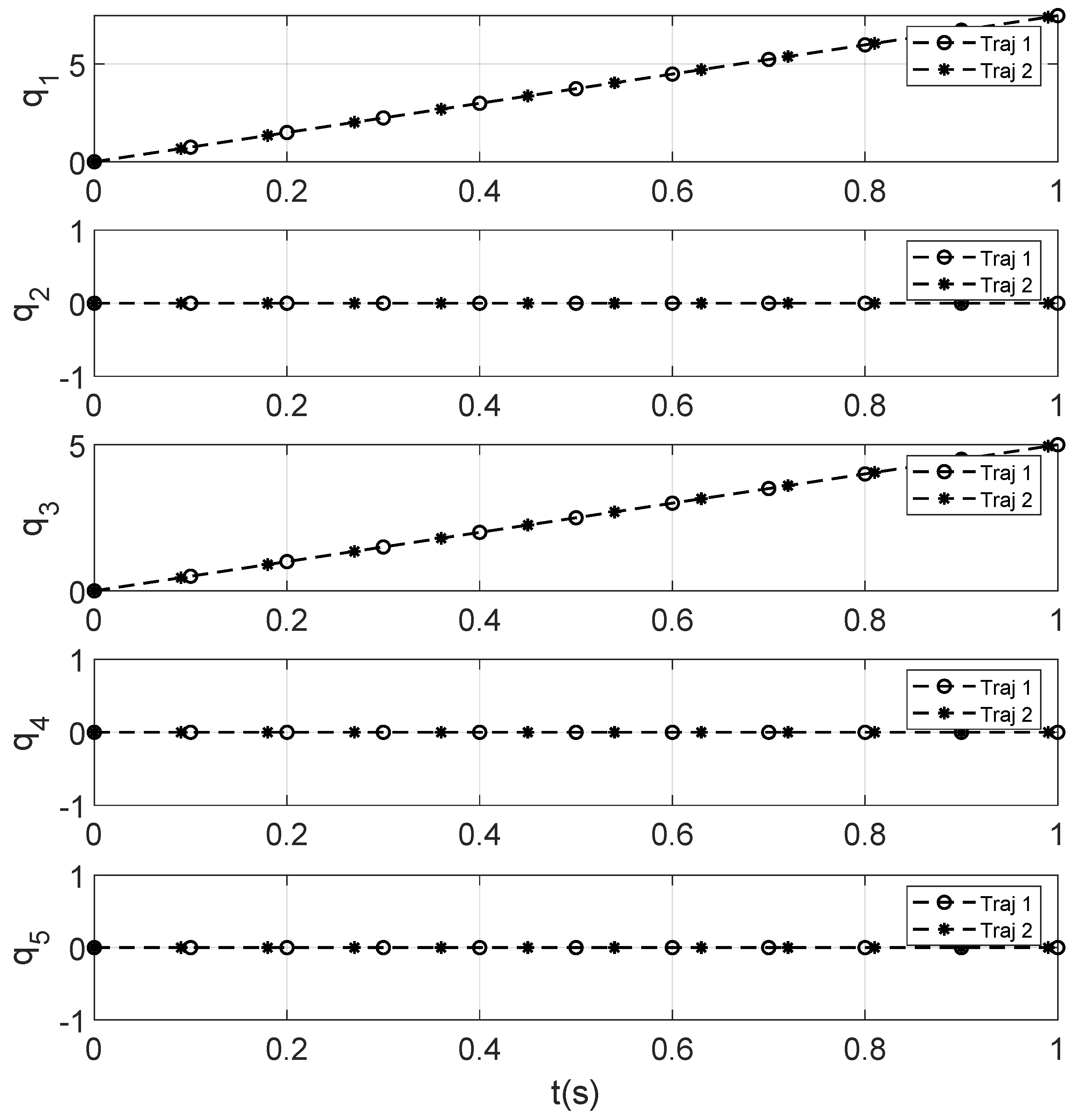
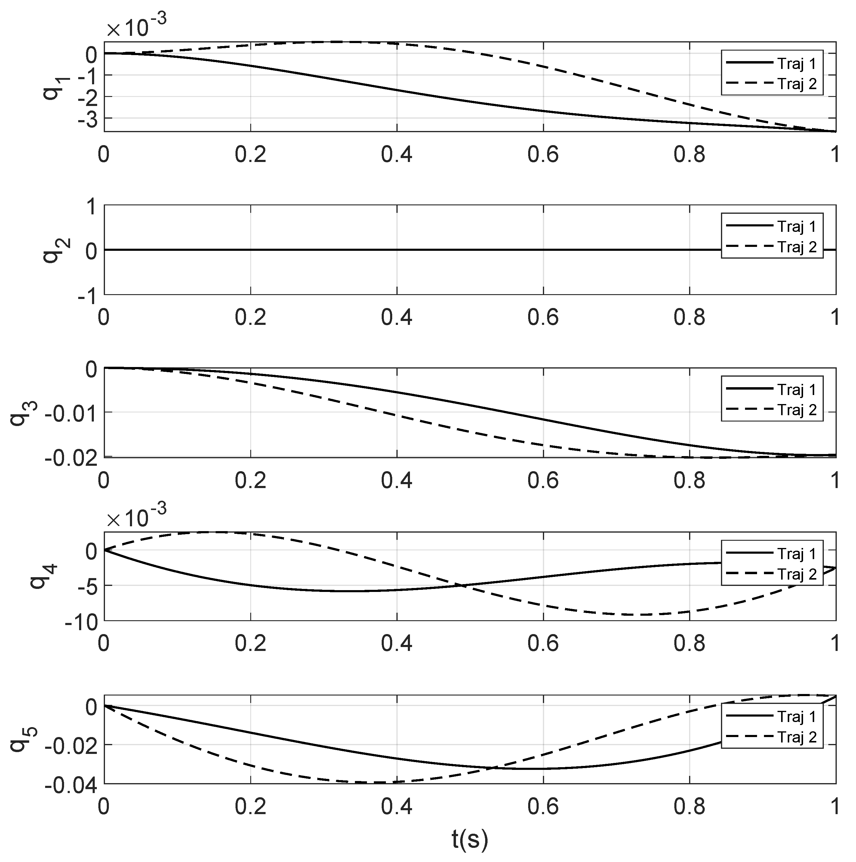
• Find the first trajectory
  Assuming the MP position is invariant to the actual trajectory length in time, we can fix the initial configuration of the system to the origin (${\mathit{q}}_{10}=\mathbf{0}$) and choose a final time $T\in {\mathbb{R}}^{+}$ as any positive real number (affecting only how fast the system passes through the optimal trajectory). We can now optimise the end point of the trajectory to be equal to the suspected Maxwell point ${\mathit{q}}_{1T}\approx {\mathit{q}}_M$. This means we choose such ${\mathit{h}}_{10}$ that drives the system to ${\mathit{q}}_M$ in time T. This is a straightforward convex minimisation task deduced from (17), since ${\mathit{q}}_{1T}$ now depends only on the choice of ${\mathit{h}}_{10}$ and no constraints are required. The cost function will take the form of a euclidean distance result in an optimisation task defined as

  $${\mathit{h}}_{10}^{*}=\underset{{\mathit{h}}_{10}\in {\mathbb{R}}^n}{arg\; min}J\left({\mathit{h}}_{10}\right)=\underset{{\mathit{h}}_{10}\in {\mathbb{R}}^n}{arg\; min}\left|\right|{\mathit{q}}_M-{\mathit{q}}_{1T}\left({\mathit{h}}_{10}\right){\left|\right|}_2^2$$

  (18)

  where ${\mathit{h}}_{10}^{*}$ is the optimal solution. The whole situation is depicted in Figure 2.
• Find the second trajectory
  Now we need to find ${\mathit{h}}_{20}^{*}$ for a second trajectory, which is different from ${\mathit{h}}_{10}^{*}$ and drives the system towards the same point ${\mathit{q}}_M$, as shown in Figure 3. We can formulate our constrained minimisation problem as (19) with constraints (20) and (21). The equality constraint (20) is meant to satisfy the same functional (9) for both trajectories.

  $${\mathit{h}}_{20}^{*}=\underset{{\mathit{h}}_{20}\in {\mathbb{R}}^n}{arg\; min}\left|\right|{\mathit{q}}_M-{\mathit{q}}_{2T}\left({\mathit{h}}_{20}\right){\left|\right|}_2^2,\mathrm{s}.\mathrm{t}.\varphi ({\mathit{y}}_1,{\mathit{y}}_2)=0\wedge \gamma ({\mathit{h}}_{10},{\mathit{h}}_{20})\le 0$$

  (19)

  $$\varphi ({\mathit{y}}_1\left({\mathit{h}}_{10}\right),{\mathit{y}}_2\left({\mathit{h}}_{20}\right))=L({\mathit{y}}_1,T)-L({\mathit{y}}_2,T)$$

  (20)

  $$\gamma ({\mathit{h}}_{10},{\mathit{h}}_{20})=-{∥\frac{{\mathit{h}}_{10}}{\left|\right|{\mathit{h}}_{10}\left|\right|}-\frac{{\mathit{h}}_{20}}{\left|\right|{\mathit{h}}_{20}\left|\right|}∥}_2^2+\rho$$

  (21)
  The parameter $\rho$ is a tuning parameter which specifies the minimal distance between the vectors ${\mathit{h}}_{10}$ and ${\mathit{h}}_{20}$, which are normalized so that the choice of this parameter is independent of their respective scales.
• Review results
  There are multiple termination conditions to the interior point algorithm. These include:
  • First-order optimality;
  • Iteration step size;
  • Number of iterations.
  Any of these can cause the algorithm to stop, but the main concern is the case where the termination occurs due to a local minimum (first-order optimality reached). If this happens, we may need to return to step 2 and restart the algorithm, giving it a different initial guess.
  To decide whether our result is valid, or if we need to restart the optimisation with a different initial guess, we can compare the value of the optimisation cost function $J\left({\mathit{h}}_{20}\right)$ with a numerical tolerance parameter. If the value is smaller than our chosen numerical tolerance, the result is valid and the Maxwell point has been confirmed.

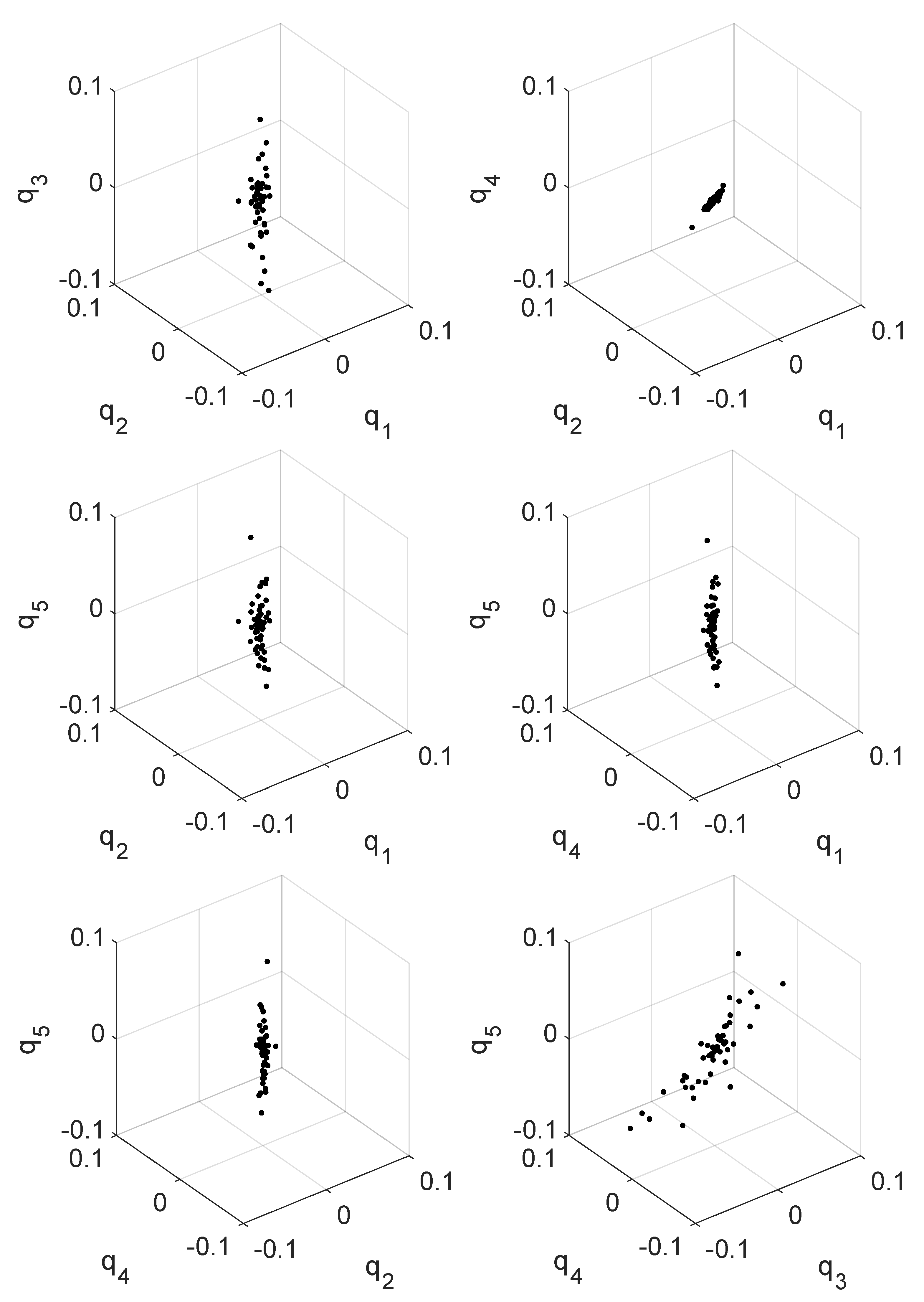
5.2. Finding MPs

In the previous section we described how to verify assumed Maxwell points, now we will describe how to find them using a similar approach. We experimented with various combinations of optimisation and random shooting and found that typical approaches such as Monte Carlo or grid search are not viable in this case because it is quite difficult to “hit” the Maxwell point exactly using shooting from random initial guesses. To overcome this issue, the task needs to be formulated as a convex optimisation problem which can converge with arbitrary precision if left iterating.

The proposed process itself is very similar to the one described in the previous section. However, in this case the location of the end point where the two trajectories intersect is unknown, so we need to optimise both ${\mathit{h}}_{10}$ and ${\mathit{h}}_{20}$ at the same time to make the end points ${\mathit{q}}_{1T}$ and ${\mathit{q}}_{2T}$ converge to a single point. This means that the dimensionality of the problem increases twofold because the number of unknown parameters is $2n$ instead of n. The whole process is shown in Figure 4, and can be described as looking for two different trajectories which start and end at the same points and have the same lengths. Based on the MP definition described earlier, if the end points do converge, we can take the end point for a Maxwell point. Formally, the optimisation task is then defined as (22), also with the constraints (20) and (21).

$$\left[\begin{array}{c}{\mathit{h}}_{10}^{*}\\ {\mathit{h}}_{20}^{*}\end{array}\right]=\underset{{\mathit{h}}_{10},{\mathit{h}}_{20}\in {\mathbb{R}}^n}{arg\; min}\left|\right|{\mathit{q}}_{1T}\left({\mathit{h}}_{10}\right)-{\mathit{q}}_{2T}\left({\mathit{h}}_{20}\right){\left|\right|}_2^2,\mathrm{s}.\mathrm{t}.\varphi ({\mathit{y}}_1,{\mathit{y}}_2)=0\wedge \gamma ({\mathit{h}}_{10},{\mathit{h}}_{20})\le 0$$

(22)

Similar to the previous section, we also need to perform an evaluation of the results through the cost function value and check whether the found minimum is truly the Maxwell point or if it is a local minimum.

After a Maxwell point is found we can restart the method with a different initial guess and repeat the process to obtain more Maxwell points. Initial guesses can be chosen randomly. It is important to note that the search process appears stochastic, and not all initial guesses are guaranteed to converge to an MP, even if they do exist. Naturally, the more initial guesses that are tried, the higher the chance of finding an MP.

When a sufficient number of Maxwell points is found, we can formulate a hypothesis about the set they form. Generally, the MPs form a subset of the full space, often a hyper-plane in linear cases. The form of the set can be analysed using standard data analysis tools such as principal component analysis or proper orthogonal decomposition (PCA) [30]. Afterwards, our hypothesis can be verified using the algorithm from the previous section applied on a new MP predicted by the hypothesis.

6. Numerical Experiments

In Section 3 and Section 4 we described the optimal control problems developed from two different approximations of the rolling disc dynamics, and in Section 5 we proposed numerical tools based on previous research [14] for analysing these control problems and finding the Maxwell points of the systems. In this section, we apply the numerical tools on both systems as case studies.

6.1. Rolling Disc—Nilpotent Approximation with Drift

Using the approximation from Section 4, based on (14), in the form of (15), the optimal control problem gives us the system of ODEs of the form

$$\dot{\mathit{q}}=\left[\begin{array}{c}\dot{q_1}\\ \dot{q_2}\\ \dot{q_3}\\ \dot{q_4}\\ \dot{q_5}\end{array}\right]=\left[\begin{array}{c}{h}_1\\ 256h_2\\ 1\\ 0\\ 0\end{array}\right],\dot{\mathbf{h}}=\left[\begin{array}{c}\dot{h_1}\\ \dot{h_2}\\ \dot{h_3}\\ \dot{h_4}\\ \dot{h_5}\end{array}\right]=\left[\begin{array}{c}0\\ -16\\ 0\\ 1\\ 0\end{array}\right]$$

(23)

This is the starting point of our numerical algorithm. We can use one more simplification based on our system of equations. The optimality functional (9) is dependent on the optimal control inputs (13). However, by calculating this we see that the resulting value of the functional is only dependent on $h_1,h_2$, which are decoupled states (states which are not dependent on any other states, only on time). This means that it is not necessary to compute the value of the resulting integral (9). If the norm of our states $h_{10},h_{20}$ is the same for both trajectories, the resulting integral value will be the same. This simplifies the constraint condition (20) into (24), where $\mathit{G}=[0,0,0,1,0]$, $\mathit{H}=[0,0,0,0,1]$.

$${\left({\mathit{G}\mathit{h}}_{10}\right)}^2+{\left({\mathit{G}\mathit{h}}_{10}\right)}^2-{\left({\mathit{H}\mathit{h}}_{20}\right)}^2-{\left({\mathit{H}\mathit{h}}_{20}\right)}^2=0$$

(24)

The algorithm was able to find some results, but the found points were not the true Maxwell points of the system. The system (23) has too many decoupled states and so there are infinitely many solutions to the minimisation problem (22) that satisfy the constraints—two trajectories have different initial vectors $\mathit{h}\left(0\right)$ and converge to the same point, but the trajectories themselves are the same. An example of such trajectories is shown in Figure 5.

6.2. Rolling Disc—Approximation Based on Taylor Linearisation

The second approximation leads us to a different set of equations (based on (11)) of the form (15).

$$\dot{\mathit{q}}=\left[\begin{array}{c}\dot{q_1}\\ \dot{q_2}\\ \dot{q_3}\\ \dot{q_4}\\ \dot{q_5}\end{array}\right]=\left[\begin{array}{c}{q}_4\\ q_3{q}_4\\ q_5\\ h_4\\ 16h_5\end{array}\right],\dot{\mathbf{h}}=\left[\begin{array}{c}\dot{h_1}\\ \dot{h_2}\\ \dot{h_3}\\ \dot{h_4}\\ \dot{h_5}\end{array}\right]=\left[\begin{array}{c}0\\ 0\\ -h_2{q}_4\\ -h_1-h_2{q}_3\\ -h_3\end{array}\right]$$

(25)

Deriving a simplification to the calculation of the optimality functional as seen in the previous section is not trivial in the case of the system (25). The final value is dependent on $h_4,h_5$, which are not decoupled, and is also dependent on other states. Therefore, in this case there is no choice but to compute the final value of the optimality functional (9) at each iteration, which increases the computational complexity.

This time, after running the optimisation, we obtain different trajectories leading to the same points (example trajectory shown in Figure 6).

In Figure 7 we can clearly see that the found points span a subspace of the original configuration space. Some dimensions in the data are numerically insignificant, forming planes or lines in specific views, see Figure 8.

To further analyse the form of the subset formed by these points, PCA analysis was performed on the data to discover the principal components in the data along with their specific latent variables which specify the amount of variance each specific component encapsulates. We can then calculated the cumulative sum of this variance for each specific number to see how many of them are needed to describe our data. This is shown in Figure 9. The calculated principal components $\widehat{\mathit{Q}}=[{\widehat{{\mathit{q}}_1}}^{\mathrm{T}}\dots {\widehat{{\mathit{q}}_5}}^{\mathrm{T}}]$ form an orthonormal basis which can be further reduced using our latent values and cumulative sum. In our case, the first 3 components describe 99.9 % of the variance in our data. So we take only the first 3 columns of the matrix $\widehat{\mathit{Q}}$ which forms a basis for our set of Maxwell points.

$${\widehat{\mathit{Q}}}_{red}=\left[\begin{array}{ccc}-0.0081& -0.0361& -0.8345\\ 0.0019& -0.0028& -0.0021\\ 0.6192& 0.7844& 0.0354\\ 0.0026& -0.0194& 0.5494\\ 0.7852& -0.6188& -0.0211\end{array}\right]$$

(26)

Note that this basis is valid only for the range of the space where the data points are available. Hypothesis based on extrapolating the data is possible but needs to be verified further.

7. Conclusions

In this paper, a numerical algorithm for finding and validating the Maxwell points of an affine control system was proposed in Section 5. The algorithm was applied to two different affine control systems, which were derived by different approximations of dynamics of the vertical rolling disc, as described in Section 6. Both of the approximations serve two purposes, that is, as a case study for the proposed numerical approach and to evaluate the effect of different approximations on the whole process of optimal control design. These numerical algorithms are the result of continuing research based on preliminary results published in [14], which proved that the Maxwell points found using numerical optimisation comply with analytical solutions.

As can be seen from the results, there are advantages and disadvantages of both derived systems. In the nilpotent-based approximation the numerical algorithm collapses to a trivial solution, as the state space trajectories are not dependent on some of the expanded states, so the optimality of the control system is lost in points different from the Maxwells ones. The problem of finding these points is much more complicated and will be part of our next research.

In opposition to this result, the common linearisation based on Taylor approximation, while still being nilpotent, yields quite different results. In this case, the numerical algorithm is able to locate a set of Maxwell points suitable for further system analyses and optimal control design. Unfortunately, the dimension of the control Lie algebra is higher than the dimension of the configuration space.

The proposed algorithms allow us, in theory, to find or validate assumed Maxwell points on any affine control system. This applies mainly in situations when analytical solutions are not available, with the only limitations being the computation power and numerical accuracy of the optimisation task. This paper only demonstrates its function on relatively simple examples, but all of the algorithm’s steps should extend well to more complicated cases, as it does not impose any insurmountable conditions on the systems being analysed. The optimisation algorithm can reach arbitrary accuracy (within reason), limited mainly by the numerical accuracy of 64-bit double precision data type. However, increasing the accuracy slows down the computation, and obtaining even a reasonable number of points can take a very long time. The task is by definition suitable for parallelisation on multiple cores of the system to reduce the computation time if needed.

Inaccuracies can also be introduced into the algorithm via integration steps of the numerical ODE solver. This is especially so if the system is stiff. For linear systems we can overcome this issue using an analytical solution to the system of ODEs, but with nonlinear systems only choosing a specialised solver or reducing the step size can solve this problem, which again trades off the computation time.

As seen in Section 6.1 there is a risk of false positives—either the system is ill defined and the constraints specified in (22) are insufficient, or a local minimum occurs when converging towards the Maxwell point. Both of these instances result in false positives and can be eliminated by checking that the point we obtained is truly a Maxwell point of the system. In the future research this problem will be addressed more concretely.

While the numerical algorithm presented in this paper is not perfect and requires understanding and interaction with the user, the results are promising and form a basis for future research.

References

- Bloch, A.M. Nonholonomic Mechanics and Control; Springer: Cham, Switzerland, 2015; p. 565. [Google Scholar]
- Frolík, S. Note on signature of trident mechanisms with distribution growth vector (4,7). In Lecture Notes in Computer Science (Including Subseries Lecture Notes in Artificial Intelligence and Lecture Notes in Bioinformatics); Springer: Cham, Switzerland, 2019; Volume 11472, pp. 82–89. [Google Scholar]
- Hildenbrand, D.; Hrdina, J.; Návrat, A.; Vašík, P. Local Controllability of Snake Robots Based on CRA, Theory and Practice. Adv. Appl. Clifford Algebras 2020, 30. [Google Scholar] [CrossRef]
- Hrdina, J.; Zalabová, L. Local geometric control of a certain mechanism with the growth vector (4,7). J. Dyn. Control Syst. 2020, 26, 199–216. [Google Scholar] [CrossRef] [Green Version]
- Hrdina, J.; Vašík, P.; Návrat, A.; Matoušek, R. Geometric Control of the Trident Snake Robot Based on CGA. Adv. Appl. Clifford Algebras 2017, 27, 633–645. [Google Scholar] [CrossRef]
- Hrdina, J.; Vašík, P.; Návrat, A.; Matoušek, R. CGA-based robotic snake control. Adv. Appl. Clifford Algebras 2016, 27, 621–632. [Google Scholar] [CrossRef]
- Hůlka, T.; Matoušek, R.; Dobrovský, L.; Dosoudilová, M. Optimization of snake-like robot locomotion using GA: Serpenoid design. Mendel 2020, 26, 1–6. [Google Scholar] [CrossRef]
- Návrat, A.; Vašík, P. On geometric control models of a robotic snake. Note Mat. 2017, 37, 119–129. [Google Scholar]
- Jurdjevic, V.; Sussmann, H.J. Control systems on Lie groups. J. Differ. Equ. 1972, 12, 313–329. [Google Scholar] [CrossRef] [Green Version]
- Agrachev, A.A.; Sachkov, Y.L. Control Theory from the Geometric Viewpoint. Encyclopaedia of Mathematical Sciences, Control Theory and Optimization; Springer: Cham, Switzerland, 2006. [Google Scholar]
- Agrachev, A.A.; Barilari, D.; Boscain, U. A Comprehensive Introduction to Sub-Riemannian Geometry; Cambridge Studies in Advanced Mathematics; Cambridge University Press: Cambridge, UK, 2019. [Google Scholar]
- Bellaïche, A.; Risler, J.J. Sub-Reimannian Geometry; Birkhäuser: Basel, Switzerland, 1996; ISBN 3034899468. [Google Scholar]
- Jean, F. Control of Nonholonomic Systems: From Sub-Riemannian Geometry to Motion Planning; Springer: New York, NY, USA, 2014; ISBN 9783319086897. [Google Scholar]
- Frolík, S.; Rajchl, M.; Stodola, M. Numerical Experiment on Optimal Control for the Dubins Car Model. In Modelling and Simulation for Autonomous Systems; Mazal, J., Fagiolini, A., Vasik, P., Turi, M., Eds.; MESAS 2020. Lecture Notes in Computer Science; Springer: Cham, Switzerland, 2021; Volume 12619. [Google Scholar] [CrossRef]
- Sachkov, Y.L.; Moiseev, I. Maxwell strata in sub-Riemannian problem on the group of motions of a plane. ESAIM Control Optim. Calc. Var. 2010, 16, 380–399. [Google Scholar] [CrossRef]
- Hrdina, J.; Návrat, A.; Zalabová, L. Symmetries in geometric control theory using Maple. Math. Comput. Simul. 2021, 190, 474–493. [Google Scholar] [CrossRef]
- Rizzi, L.; Serres, U. On the cut locus of free, step two Carnot groups. Proc. Am. Math. Soc. 2017, 145, 5341–5357. [Google Scholar] [CrossRef]
- Monroy-Pérez, F.; Anzaldo-Meneses, A. Optimal Control on the Heisenberg Group. J. Dyn. Control. Syst. 1999, 5, 473–499. [Google Scholar] [CrossRef]
- Bucolo, M.; Buscarino, A.; Famoso, C.; Fortuna, L.; Frasca, M. Control of imperfect dynamical systems. Nonlinear Dyn. 2019, 98, 2989–2999. [Google Scholar] [CrossRef]
- Najman, J.; Brablc, M.; Rajchl, M.; Bastl, M.; Spáčil, T.; Appel, M. Monte Carlo Based Detection of Parameter Correlation in Simulation Models. In Mechatronics 2019: Recent Advances towards Industry 4.0; Advances in Intelligent Systems and Computing; Springer: Cham, Switzerland, 2020; ISBN 978-3-030-29992-7. [Google Scholar] [CrossRef]
- Rubes, O.; Brablc, M.; Hadas, Z. Nonlinear vibration energy harvester: Design and oscillating stability analyses. Mech. Syst. Signal Process. 2019, 125, 170–184. [Google Scholar] [CrossRef]
- Bloch, E.D. A First Course in Geometric Topology and Differential Geometry; Birkhauser: Boston, MA, USA, 1997; ISBN 3764338407. [Google Scholar]
- Hrdina, J.; Vašík, P. Notes on differential kinematics in conformal geometric algebra approach. In Advances in Intelligent Systems and Computing; Springer: Cham, Switzerland, 2015; Volume 378, pp. 363–374. [Google Scholar] [CrossRef]
- Štefek, A.; Pham, V.T.; Křivánek, V.; Pham, K.L. Energy comparison of controllers used for a differential drive wheeled mobile robot. IEEE Access 2020, 8, 170915–170927. [Google Scholar] [CrossRef]
- Dubins, L.E. On curves of minimal Length with a constraint on average curvature, and with prescribed initial and terminal positions and tangents. Am. J. Math. 1957, 79, 497–516. [Google Scholar] [CrossRef]
- Ascher, U.M.; Petzold, L.R. Computer Methods for Ordinary Differential Equations and Differential-Algebraic Equations; Society for Industrial and Applied Mathematics: Philadelphia, PA, USA, 1998; ISBN 978-0-89871-412-8. [Google Scholar]
- Press, W.H.; Teukolsky, S.A.; Vetterling, W.T.; Flannery, B.P. Section 18.1. The Shooting Method. In Numerical Recipes: The Art of Scientific Computing, 3rd ed.; Cambridge University Press: New York, NY, USA, 2007; ISBN 978-0-521-88068-8. [Google Scholar]
- Boyd, S.; Vandenberghe, L. Convex Optimization; Cambridge University Press: Cambridge, UK, 2004. [Google Scholar]
- MathWorks, Constrained Nonlinear Optimization Algorithms. Available online: https://www.mathworks.com/help/optim/ug/constrained-nonlinear-optimization-algorithms.html (accessed on 13 March 2021).
- Jolliffe, I.T. Principal Component Analysis; Springer Series in Statistics; Springer: New York, NY, USA, 2002; ISBN 978-0-387-95442-4. [Google Scholar] [CrossRef]