Abstract
The daily lifestyle of an average human has changed drastically. Robotics and AI systems are applied to many fields, including the medical field. An autonomous wheelchair that improves the degree of independence that a wheelchair user has can be a very useful contribution to society. This paper presents the design and implementation of an autonomous wheelchair that uses LIDAR to navigate and perform SLAM. It uses the ROS framework and allows the user to choose a goal position through a touchscreen or using deep learning-based voice recognition. It also presents a practical implementation of system identification and optimization of PID control gains, which are applied to the autonomous wheelchair robot. Input/output data were collected using Arduino, consisting of linear and angular speeds and wheel PWM signal commands, and several black-box models were developed to simulate the actual wheelchair setup. The best-identified model was the NLARX model, which had the highest square error (0.1259) among the other candidate models. In addition, using MATLAB, Optimal PID gains were obtained from the genetic algorithm. Performance on real hardware was evaluated and compared to the identified model response. The two responses were identical, except for some of the noise due to the encoder measurement errors and wheelchair vibration.
1. Introduction
Nowadays, Autonomous Mobile Robots (AMRs) play an important role in a wide range of applications and fields, including, but not limited to, institutions, airports, malls, hospitals, and factories. AMR is a type of robot that is programmed to avoid obstacles and perform complex tasks in flexible and intelligent ways with little human interaction, so it can be considered an innovative technology able to improve efficiency and ensure precision, enhance speed, and increase safety in many fields [1]. AMRs usually operate in an unknown and unpredictable environment, so they are designed to be capable of understanding, scanning, and navigating the surrounding environment, thus differing from Autonomous Guided Vehicles (AGVs), which rely on a predefined path and physical guidance [2,3,4]. Multiple AMRs, called Multi-Agent Robot Systems (MARSs), can perform complex missions by distributing the tasks and sharing data between multiple collaborating robots physically engaged with each other, providing the benefits of reduced time and energy consumption, robustness, and efficiency of the system, achieving better results than each robot individually [5,6,7,8].
AMRs use a sophisticated set of sensors and actuators, and different types of control algorithms to perform various tasks, such as obstacle avoidance (OA) [9,10,11,12], navigation [13,14], and simultaneous localization and mapping (SLAM) [15,16,17,18]. SLAM is a method where the robot builds a 2D map of an unknown environment and simultaneously localizes itself in that map. Then, it can plan the shortest collision-free path to its location goal [19]. Hence, the robot’s positioning is an important aspect for the tasks AMRs can perform, either indoors or outdoors. There are various sensors used to collect data for the abovementioned tasks, such as cameras [20,21,22], depth sensors [23], LIDAR [21,24], laser range sensors [17,25], and ultrasonic sensors [26,27]. After collecting the data from the robot, then comes the issue of making it able to direct itself from the current position to the desired destination following the predefined path. This is the control algorithm’s role. Different control strategies have been proposed to control the robot’s trajectory planning. Path planning and robot motion can be controlled by classical control methods such as PID/PI controller [28,29,30]; modern control methods such as fuzzy control [31,32]; the visual odometry technique, which estimates the robot’s movement in the third dimension and updates the robot’s position continuously [1]; deep reinforcement learning (DRL), which can deal effectively with uncertain environments [2]; and several optimization algorithms, such as the Kalman filter [18,33,34] and genetic algorithms [35,36]. The construction of control rules for the angular, linear, and acceleration of the nonholonomic wheeled mobile to trace the desired path is the control problem for trajectory tracking. The control strategy seeks to reduce the discrepancy between the intended and actual track. Sensor errors that are measured from both internal and external sources are the cause. Additionally, slippage, disruptions, and noise are to blame. The nonholonomic constraint prevents the mobile robot from moving quickly in the direction orthogonal to its wheel axis.
Advanced control methods, including adaptive control, variable structure control, fuzzy control, and neural networks, can be used to solve this issue. Implementing self-tuning adaptive control systems presents many challenges, including the inability to maintain trajectory control in the midst of jarring disruptions or loud noises. This is due to the possibility that the parameter estimator could produce false findings in the face of jarring shocks or significant noise. The implementation of a variable structure controller is simple but challenging. This is due to the potential for a sudden shift in the control signal, which could have an impact on how the system functions [37]. Although it takes greater computer power and data storage space, a neural-network-based motor control system has a strong ability to solve the system’s structure uncertainty and disturbance [38]. The majority of the time, fuzzy control theory offers nonlinear controllers that can execute a variety of complicated nonlinear control actions, even for uncertain nonlinear systems [39]. An FLC does not necessitate exact knowledge of the system model, such as the poles and zeroes of the system transfer function, unlike conventional control designing [40]. Fewer calculations are required by a fuzzy logic control system based on an expert knowledge database, but it is unable to accommodate the new rules. The fundamental challenge in using conventional PID controllers is selecting the control parameters accurately [41]. Random or even manual configuration of these control parameters may result in the system not responding as anticipated, especially when there are system uncertainties [42,43]. Only when the plant model is defined as first-order with dead time is the Ziegler–Nichols method used. Algorithms for optimization have recently been created. Examples include fruit fly optimization, particle swarm optimization, and genetic algorithms (GAs) (FFO) [44]. In [45], GA optimization is used to find the optimal PID control parameters for a multi-input multi-output (MIMO) nonlinear system for the twin rotor of the helicopter.
This paper is an extension of the work in [33]. Real input/output data are collected experimentally from a six-wheel autonomous differential wheelchair that operates a SLAM task. The robot wheelchair uses different input devices, indicating its ability to operate in both manual and automatic modes, such as a joystick for speed/position control, an ultrasonic sensor for detecting and avoiding obstacles, and a PRLIDAR (SLAMTECH, Shanghai, China) sensor for map construction, and it is controlled using an ROS framework that allows the user to choose the predefined goal position by using the touchscreen or voice recognition mode. Right and left wheel PWM signals are measured using feedback encoders taken as the input data. Two system identification methods are estimated using the collected data with Matlab software version 9.9 (US). Several candidate models are designed to simulate the actual wheelchair, and a SIMULINK model is obtained to build a closed-loop form using the PID control. Two PID controllers are used where one of them is for the robot’s linear speed control and the other is for angular speed control, and their output is applied to the kinematics equations of the differential drive mobile robot. Tuning these PID controllers can be achieved using trial and error, which can consume a large amount of time, so this paper presents one of the alternative and more accurate methods, the genetic algorithm (GA) optimization method, to find the optimal PID gains, and a comparison between the performance of the estimated model and the actual robot is obtained based on experimental results.
The paper is prepared as follows. Firstly, the experimental setup is presented. Secondly, system identification is explained. Thirdly, the proposed controller techniques are demonstrated. Fourthly, the experimental results are illustrated. Finally, the conclusion is discussed. The paper is prepared as follows. Firstly, the experimental setup is presented. Secondly, system identification is explained. Thirdly, the proposed controller techniques are demonstrated. Fourthly, the experimental results are illustrated. Finally, the conclusion is discussed.
2. Autonomous Wheelchair Experimental Setup
2.1. Experimental Setup Structure
In this design, the wheelchair would be working with a six-wheel chassis to make it easier to rotate in a 360-degree circle and flexible enough to move indoors and outdoors. Some pipes are used in this design to free up space in the middle and make a box for batteries and controllers. The wheelchair contains two electrical control boxes fixed inside the chassis, as shown in Figure 1. Control box 1 consists of two lead acid batteries, a buck converter, three batteries with 3.5 volts each, and a battery charging circuit. Control box 2 encloses Arduino mega 2560, Raspberry Pi 3, motor driver, and power terminal PCB. The final design is made from a pipe system connected by joints. Two fixed wheels, four freewheels, a chair made from leather, and head support are included. In addition, the wheelchair system was enhanced with RPLIDAR sensor to allow it to make a map while moving, with eight ultrasonic sensors for obstacle avoidance purposes, and two feedback encoders coupled with the motors.
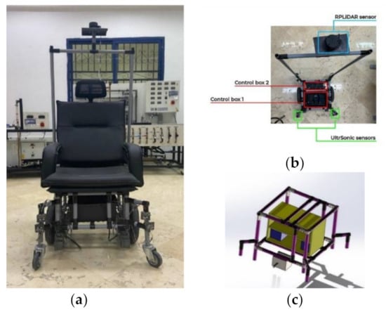
Figure 1.
The experimental wheelchair setup: (a) the front view of the experimental wheelchair; (b) the top view of the experimental wheelchair; (c) the solid work design.
Arduino Mega is used as a data acquisition device, and pulses are counted using Arduino built-in Interrupts. For each sample (50 ms), the distance that each wheel has traveled can be expressed as
where is the traveled distance, is the wheel diameter and is the pulse per revolution. Then, encoder_pulses_count is set to zero at each sample, so that the difference is only recorded in each loop to save memory, and the Int32 message is used due to the high number of pulses of the high-resolution encoder.
After determining the distance each wheel has traveled (, it is the center of the robot that is of interest. This complies with the Unicycle model kinematics illustrated in Equation (2); the distance traveled by the center of the robot is taken as the average of distance traveled by the two wheels.
The angle θ, representing the robot’s orientation, can then be defined as shown in Equation (3), where is defined as the distance between the two wheels of the robot. It is assumed that the robot always moves in a planar 2D motion so the angle θ is about the z axis.
The position and orientation of the robot can be expressed as a vector of displacements in the x and y directions, and the angle θ defines the orientation.
As follows and the absolute position of the robot can be expressed as
Velocities ( is the velocity in the x direction; is the velocity in the direction and is the rotational velocity) can be calculated accordingly by dividing the change in position vector, and substituting it will obtain
Figure 2 shows the kinematics of the differential drive mobile robots, illustrating some of the parameters used.
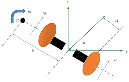
Figure 2.
Robot Kinematics.
2.2. Wheelchair Mathematical Model
Consider a nonlinear MIMO system of the form:
The MIMO system has a vector relative degree (ρ1, ρ2, ..., ρm) if the following matrix is nonsingular:
where
The system can be represented in the form:
For the trajectory tracking problem, the natural outputs of the system are:
Therefore,
Let us assume that the relative degree of the system is (ρ1, ρ2) = (1, 1).
We conclude that A(p) is singular, and the relative degree is not (1, 1). The problem is that the input u1 or v appears in the derivative of both outputs, while the input u2 (or ω) does not.
Let us try to make v appear later in a higher-order derivative of the output.
The new representation of the system is
v appears in the derivative of both outputs. ω does not appear in the derivative of any output.
The new system with the extended state is:
In a compact form
where
The inputs do not appear in the first-order derivative of the outputs. Let us see the second-order derivatives.
First, we have to calculate Lf h1(p) and Lf h2(p):
Now we calculate the entries of A(p):
Therefore, A(p) is given by
3. System Identification
Using experimental input and output data, system identification aims to establish the model system’s parameters. There are three fundamental steps in the process of developing a model. The input and output data come first. This information is gathered through the experiment. The set of candidate models comes next. From the pool of potential models, we must study the most suited model.
The general linear transfer function of the wheelchair system may be written as the following Equations (47) and (48).
where is the linear speed of the wheelchair, is the angular speed of the wheelchair, is the input voltage for the right motor, and is the input voltage for the left motor. The n is the system order and, , , and are the estimated parameters of the approximate transfer function.
It is well-known that linear models cannot accurately describe a nonlinear system [3]. By raising the order of the linear system, the model’s accuracy can be improved. However, it is frequently the case that increasing order is unable to substantially increase model accuracy. As a result, the nonlinearities (such as friction and backlash) must be explicitly included in the system [16].
In this study, we attempt to model such systems using the nonlinear ARX model structure, where AR denotes the autoregressive portion and X denotes the additional input. As seen in Figure 3, a nonlinear ARX model can be thought of as an expansion of a linear model.
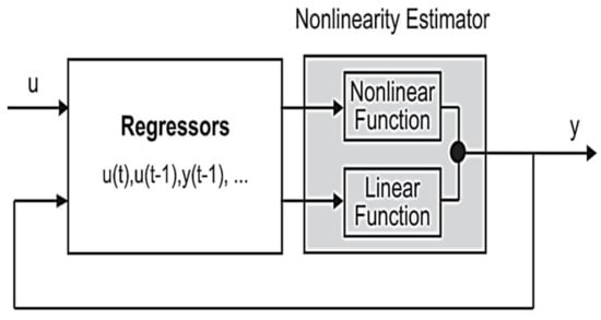
Figure 3.
The structure of a nonlinear ARX model.
These models are defined as those that have a nonlinear dependence on their parameters. For example, see Equation (49).
To illustrate how this is achieved, first the relationship between the nonlinear equation and the data can be expressed generally as
where is a measured value of the dependent variable, is a function of the independent variable and a nonlinear function of the parameters , and is a random error.
This model can be expressed in an abbreviated form by omitting the parameters
The nonlinear model can be expanded in a Taylor series around the parameter values:
where j = the initial guess, j + 1 = the prediction, , and , and substituting Equation (51) into Equation (52) will result in Equation (53).
or in matrix form
where is the matrix of partial derivatives of the function evaluated at the initial guess j,
where n = the number of data points.
The vector {D} contains the differences between the measurements and the function values,
The vector contains the changes in the parameter values,
Applying linear least-squares theory to Equation (10),
for {∆H}, which can be employed to compute improved values for the parameters, as in
Two input/two output data had been collected using Arduino and ROS. The right and left motors receive a PWM command ranging from −255 to 255 as demonstrated in Figure 4. The output position and orientation data are calculated using differential drive robot kinematics equations as follows: each motor has an Omron E6B2-CWZ6C incremental rotary encoder that provides 2000 PPR resolution with two channels 90o out of phase to determine the direction of rotation. The collected data are summarized in Figure 5.
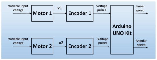
Figure 4.
Block diagram of wheelchair through open-loop mode.
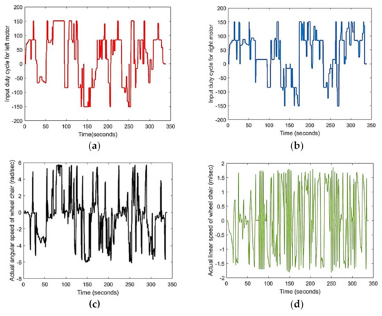
Figure 5.
The collected input/output data from the wheelchair are listed as: (a) input duty cycle for left motor; (b) input duty cycle for right motor; (c) actual angular speed of wheelchair; (d) actual linear speed of the wheelchair.
A black box that takes two inputs and two outputs is needed. A MIMO model was estimated using the system identification toolbox to adapt to the nonlinearities in the mapping from inputs to outputs. The NLARX model will be used and compared with three-transfer function models (three poles and two zeros, six poles and three zeros, twelve poles and six zeros) (Appendix A). The NLARX could achieve a lower mean squared error and was more suitable to use with SIMULINK for optimizing PID controller gains, as demonstrated in Table 1.

Table 1.
The mean square error of obtained identified model.
Figure 6 shows the four models’ comparison and fitness to training data. Transfer function models were better at estimating the angular speed output but could not capture the relation between inputs and the linear speed; thus, we used the NLARX model. It can noted that the zoomed-in area confirms that the NLARX model can track the actual behavior of the wheelchair experimental setup.
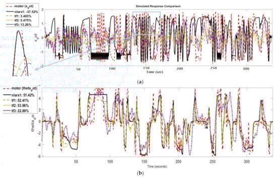
Figure 6.
The actual response of the wheelchair mobile robot and the candidate identified models’ responses: (a) the linear motion response; (b) the rotational motion response.
4. GA-Based PID Control
The transfer function of the PID controller is , where ,, are proportional, integral, and differential gains, respectively. Each component of a PID controller serves the following purpose: the proportional component lowers the system’s error reactions to disturbances, the integral component removes the steady-state error, and the derivative component dampens the dynamic response and increases system stability [8]. Selecting the three parameters for the PID controller that are appropriate for the controlled plant is a challenge. There are other ways to establish the PID controller’s parameters, such as Ziegler–Nichols and trial-and-error; however, the majority of these approaches are unreliable. The GA serves as a tool for various design processes to solve complex optimization challenges. It overcomes the problems with traditional optimization methods, such as using broad ranges rather than generating millions of probabilities to obtain the optimum function. Convergence is slow and occurs at local minima and maxima based on an educated guess. Calculation of derivatives takes time. Additionally, the GA does numerous parallel optimum point searches. So, the parameters for PID controllers were found using distinct cost function genetic algorithm techniques in this work.
This cost function as shown in Equation (60) minimizes the integrated square error e(t).
The systematic diagram for the wheelchair in a closed-loop form is illustrated in Figure 7. It can be noted that the system consists of two PID controllers. The first is for the angular speed, and the second is for the linear speed. In addition, the output of the controllers is a pulse width modulation (PMW) which can adapt to the motor speed.
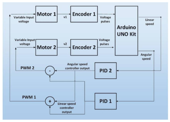
Figure 7.
The block diagram of the wheelchair in a closed-loop form.
A highly helpful technique for searching and optimizing a variety of engineering and scientific challenges is the genetic algorithm (GA). In this thesis, the GA is used to adjust the PID controller parameters in order to employ distinct cost functions to identify the best solutions. Here, we model it using the MATLAB Genetic Algorithm Toolbox. The first and most important stage is to encode the issue onto the appropriate GA chromosomes, followed by population construction. Some studies advise having 20–100 chromosomes per population. The likelihood of obtaining the best outcomes will increase with the number of chromosomes. We employ 80 chromosomes in each generation, though, because we have to take the execution time into account.
The six parameters , ,, , , and of each chromosome have different value constraints depending on the cost functions utilized. In order to achieve the best results, the starting values of , , , , , and are derived from the Ziegler–Nichols rule. According to Equation (61), the population in each generation is represented by an 80 × 7 matrix, depending on the population’s chromosomal count.
where n: number of chromosomes.
Each row is one chromosome that comprises , , , , , and values, and the last column is added to accommodate fitness values (F) of corresponding chromosomes. The final values of , , , , , and are determined by minimizing a certain cost function, as demonstrated in Figure 8.
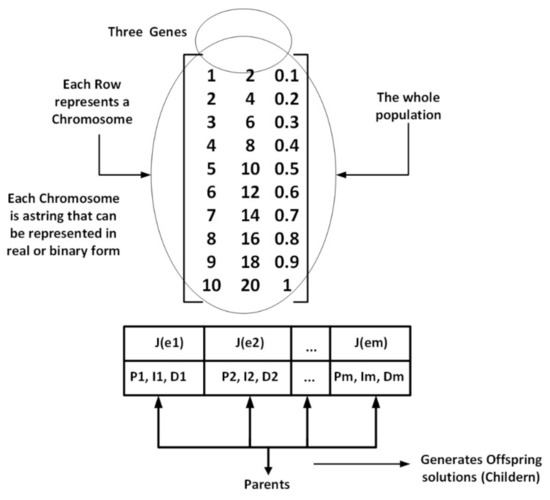
Figure 8.
The GA optimization tuning process.
The GA steps can be summarized as follows: the first step is selecting the search interval. This stage necessitates knowledge, experimentation, or assumption based on the system eigenvalues that characterize the system stability region. In the second step, the population is created at random inside the search window. In the third step, based on the cost function, chromosomes from the present generation (population) are chosen (reproduced) to be parents to the following generation. In the fourth step, children’s new chromosomes retain a lot of their parents’ traits.
Having a model to control, we applied PID controllers using the same scheme used with the Arduino; that is, one PID takes on the linear speed error, and another one handles the angular speed error. Then, the optimization was applied using the genetic algorithm and the Integral Time Weighted Absolute Error, ITAE, as an objective function.
The resulting PID gains were as follows for the linear speed PID = 64.3182, = 5.6344, = 4.0823) and for the angular speed PID = 40.061, = 24.0089, = 1.0923).
5. Experimental Results
This section illustrates the experimental results where the obtained parameters of the PID’s controllers will be applied practically and then compared with the simulated results with MATLAB Simulink to validate the identified model. In addition, the navigation experiment results will be presented. Figure 9 demonstrates a comparison between the wheelchair linear and angular speed responses in two cases. The first case considers the response of the identified model based on the NLARX model. The second case is the actual autonomous wheelchair response. It can be noted that the actual response is approximately identical to the simulated results, which ensures that the obtained identified model is accurate and can simulate the actual autonomous wheelchair. Moreover, the actual response suffers from shuttering due to the measured signal noise of the encoder and wheel vibration.
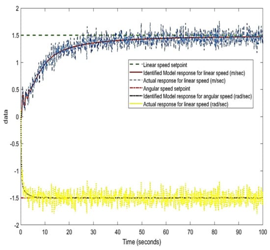
Figure 9.
The linear and angular speed for both the identified model and the actual wheelchair.
Autonomous robot navigation refers to giving the robot a goal position inside a map, and the robot should move from its initial position to the goal position without any input from the user, achieving the constraint of following the shortest and safest collision-free path, as well as parameter constraints such as when accelerations and velocities are limited within a certain range. Autonomous navigation requires a number of tasks to be performed. Figure 10 summarizes the subproblems in autonomous navigation, along with some famous algorithms that solve these problems.
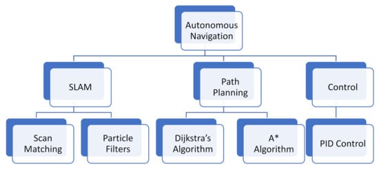
Figure 10.
The subproblems in autonomous navigation, along with some famous algorithms.
The navigation methodology steps of the wheelchair is demonstrates in Figure 11.
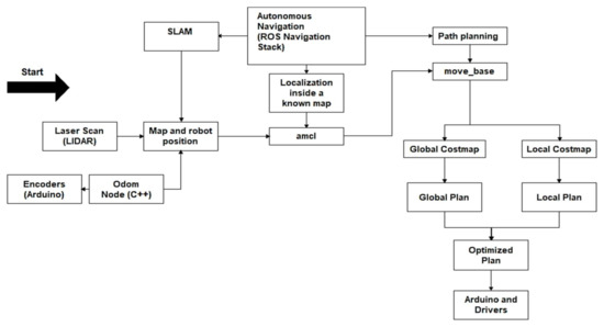
Figure 11.
The block diagram of the navigation steps for the autonomous wheelchair.
For a robot to autonomously navigate in an unknown environment, it needs to localize itself inside this environment and find out what this environment looks like at the same time, a problem referred to as the simultaneous localization and mapping problem, or SLAM for short. SLAM is a well-known problem in robotics, and many approaches to solving it have been made. Scan matching algorithms, such as hector_slam, are one of the algorithms of interest, as an implementation of this algorithm is available as an open-source ROS package. Scan matching makes use of the high scanning rate of modern laser scanners; it tries to align new scans with the existing map built from previous scans to best describe the environment and find the robot’s position. hector_slam uses Gauss–Newton optimization to align the scans with each other; the coordinates of the scan endpoints are a function of the robot’s position in the world, which is described using a rigid transformation as follows:
where represents the robot’s pose and is the vector representing the scan endpoint coordinates, in 2D. hector_slam aims to find the transformation described by which would best align the new scans to the map built from the previous scans, which also represents the robot’s position and is represented by
where returns the map value at the given coordinates of .
A famous representation of maps used in robotics is grid occupancy maps, where maps consist of grid cells that hold the probability of each cell being occupied. After the robot has built its map and found itself inside it, it is given a goal position to move to; starting from an estimated initial position, path planning algorithms find the shortest path to follow that is collision-free. A famous algorithm that is used to find the shortest path between two points is Dijkstra’s algorithm. The algorithm finds the shortest distance to all points from the starting point, which is computationally inefficient. An improvement of Dijkstra’s algorithm is the A* algorithm, which uses the same principles but adds a heuristic function to the algorithm; this allows the algorithm to find a path that may not be optimal, but is good enough, and does that much faster in terms of computational time.
With the knowledge of the set of points that the robot must follow with certain velocities, the path, there must a low-level controller that makes sure the robot’s linear and angular speeds are correctly updated and adjusted to track the given path. This is the most significant contribution of our work.
Input from the user is given using a GUI that is shown on a 5” touchscreen, which we use as our desktop environment. A photo of our simple, proof-of-concept GUI is shown next (Figure 12).
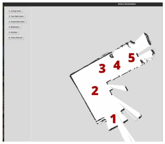
Figure 12.
Simple GUI built using the Tkinter Python library.
The user can select one of the places as the go-to destination, and predetermined position and orientation inside the destination are then sent to the ROS navigation stack as a new navigation goal. As for the ease-of-access feature, we added the ability to choose the destination number using voice recognition. We used a TensorFlow [2] deep learning library to build a speech command recognition model that recognizes digits 0–9. The model was trained on the public speech command dataset [3]. The model was converted to the tf.lite format to be able to perform inference on the Raspberry Pi.
Using the LIDAR, and after having the odometry and required transforms ready, navigation trials started. Using the hector slam package, multiple maps of different environments were created, and we faced a problem in that sometimes the map became distorted, which affected the navigation stack performance.
Figure 13 shows a map of the workshop created by hector slam. Figure 12 also shows an example of the maps becoming distorted, depending on how the robot is moved and how the scanning occurs. As a solution to this problem, we tried to use Gmapping to perform a SLAM alternative to hector slam. Although it achieved better maps, Gmapping uses Odometry as opposed to hector slam, which means it is highly affected by the encoder reading, which has noise.
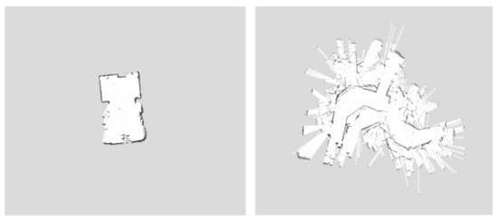
Figure 13.
Two maps created by hector_slam showing the occurrence of case distortion.
Figure 14 shows some of the experiments using the ROS navigation stack. The robot planned a global path and a local path to arrive at the given goal; however, the performance was not accurate, as the navigation stack requires many parameters to be set, and more tuning was needed.
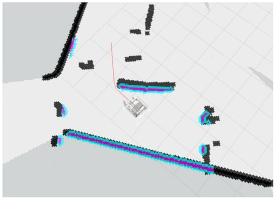
Figure 14.
RVIZ showing robot model receiving navigation goal.
Navigation testing proceeded by gathering parameters from the LIDAR (SLAMTECH, China) sensor and the encoder to properly perform navigation. An issue during testing was that once synchronization was lost between the Arduino and Raspberry Pi, the wheelchair activated recovery behavior mode. It may move in a circular path around its center or try to find the path with the least obstacles to move on. Another issue was that obstacles appearing on the map remained on the map. This issue caused the errors in navigation and the path planning process. Moreover, once in recovery mode, the wheelchair might start to rotate around itself as obstacles remain around it on the map. The autonomous mode was tested in an indoor environment. A map was built by the robot using the hector slam mapping package. It was then loaded by the map server package and received by the amcl localization package, and moved base to perform the navigation goal. Figure 15 displays the room where tests were conducted. Features of the map generated are highlighted and shown in Figure 16.
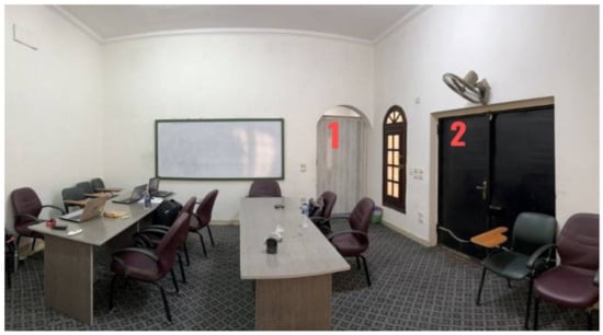
Figure 15.
The area used in testing the navigation, where positions 1 and 2 are marked.
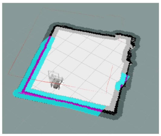
Figure 16.
Map of the area scanned.
Costmaps were performed by the move_base package. Figure 17 shows the global costmap and the local costmap, highlighted in the blue color scheme.
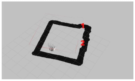
Figure 17.
Stack of the static map, global map, and the local map layers above each other.
First, navigation trials showed that move_base parameters needed more tuning, especially the speed and acceleration limits. The robot was taken to several different areas to proceed with testing. The navigation system showed great results in wide areas; however, in smaller areas and narrow paths, the results show the need for extra testing and tunning of the navigation stack parameters.
6. Conclusions
This paper presents practical steps to develop an identified model for an autonomous wheelchair system that considers a multi-input multi-output system. Input/output data were collected from an autonomous differential drive wheelchair controlled using the ROS framework, taking as input the right and left wheel PWM command. These data were used to estimate a black-box model using MATLAB, where several candidate models were obtained to find the best among them. Two methods of system identification were used; the first was linear least square with different orders while the second method was the nonlinear least square. The comparison between the candidate models made it obvious that the identified model based on the NARX was the best. A closed-loop form using two PID controllers was built where one of them controls the linear speed of the robot, and the other one controls the angular speed. The genetic algorithm (GA) was used to find the optimal PID gains based on a certain cost function. The obtained parameters were applied to the identified model and the actual system. The results show that the two responses are nearly identical. Several input devices were used as speed/position references, such as voice recognition, joystick (manual mode), and a LiDAR sensor (autonomous mode). Additionally, it uses the ROS (Version 2, US) framework and allows the user to choose a goal position. The results show that the performance of the autonomous wheelchair had been improved.
Author Contributions
Data curation, A.Y.; Formal analysis, D.M.; Investigation, A.E.; Methodology, M.A.S.; Project administration, M.A.S. and M.B.; Resources, S.A.; Software, E.K. and A.H.; Supervision, M.A.S. and M.B. All authors have read and agreed to the published version of the manuscript.
Funding
This research was funded by Future University in Egypt.
Institutional Review Board Statement
Not applicable.
Informed Consent Statement
Not applicable.
Data Availability Statement
Not applicable.
Conflicts of Interest
The authors declare no conflict of interest.
Appendix A
The first transfer function is as follows.
The second transfer function is as follows.
The third transfer function is as follows.
The fourth model, NARX, is as follows. larx1 = nonlinear ARX model with two outputs and two inputs. Inputs: vr, vl, Outputs: x_dot, theta_dot Standard regressors corresponding to the orders: na = [2 0; 0 2], nb = [2 2; 2 2], nk = [1 1; 1 1]. For output 1: x_dot(t−1), x_dot(t−2), vr(t−1), vr(t−2), vl(t−1), vl(t−2). For output 2: theta_dot(t−1), theta_dot(t−2), vr(t−1), vr(t−2), vl(t−1), vl(t−2). Nonlinearities: For output 1: wavenet with 38 units, For output 2: wavenet with 3 units. Sample time: 0.05 s
References
- Raharja, N.; Ma’arif, A.; Adiningrat, A.; Nurjanah, A.; Rijalusalam, D.; Sánchez-López, C. Empowerment of mosque community with ultraviolet light sterilisator robot. J. Pengabdi. Dan Pemberdaya. Masy. 2021, 1, 95–102. [Google Scholar]
- Paola, D.D.; Milella, A.; Cicirelli, G.; Distante, A. An autonomous mobile robotic system for surveillance of indoor environments. Int. J. Adv. Robot. Syst. 2010, 7, 19–26. [Google Scholar] [CrossRef]
- Murthy, V.M.; Kumar, S.; Singh, V.; Kumar, N.; Sain, C. Autonomous mobile robots designing. J. Glob. Res. Comput. Sci. 2011, 2, 126–129. [Google Scholar]
- Nurmaini, S.; Tutuko, B. Intelligent Robotics Navigation System: Problems, Methods, and Algorithm. Int. J. Electr. Comput. Eng. 2017, 7, 3711–3726. [Google Scholar] [CrossRef][Green Version]
- He, W.; Krupa, A.; Li, Z.; Chen, C.P. A Survey of Human-centered Intelligent Robots: Issues and Challenges. IEEE/CAA J. Autom. Sin. 2017, 4, 602–609. [Google Scholar] [CrossRef]
- Boudra, S.; Berrached, N.-E.; Dahane, A. Efficient and secure real-time mobile robots cooperation using visual servoing. Int. J. Electr. Comput. Eng. (IJECE) 2019, 10, 3022–3034. [Google Scholar] [CrossRef]
- Rasheed, A.A.A.; Abdullah, M.N.; Al-Araji, A.S. A review of multi-agent mobile robot systems applications. Int. J. Electr. Comput. Eng. (IJECE) 2022, 12, 3517–3529. [Google Scholar] [CrossRef]
- Manikandan, N.; Kaliyaperuma, G. Collision avoidance approaches for autonomous mobile robots to tackle the problem of pedestrians roaming on campus road. Pattern Recognit. Lett. 2022, 160, 112–121. [Google Scholar] [CrossRef]
- Alatise, M.B.; Hancke, G. A Review on Challenges of Autonomous Mobile Robot and Sensor Fusion Methods. IEEE Access 2020, 8, 39830–39846. [Google Scholar] [CrossRef]
- Wahyono, E.P.; Ningrum, E.S.; Dewanto, R.S.; Pramadihanto, D. Stereo vision-based obstacle avoidance module on 3D point cloud data. Telecommun. Comput. Electron. Control. 2020, 18, 1514–1521. [Google Scholar] [CrossRef]
- DAS, S.K. Local path planning of mobile robot using critical-point bug algorithm avoiding static obstacles. IAES Int. J. Robot. Autom. (IJRA) 2016, 5, 182–187. [Google Scholar] [CrossRef]
- Hayet, T.; Jilani, K. A navigation model for a multi-robot system based on client/server model. In Proceedings of the International Conference on Control, Decision and Information Technologies 2016, Saint Julian’s, Malta, 6–8 April 2016. [Google Scholar]
- Abdulredah, S.H.; Kadhim, D.J. Developing a real time navigation for the mobile robots at unknown environments. Indones. J. Electr. Eng. Comput. Sci. (IJEECS) 2020, 20, 500–509. [Google Scholar] [CrossRef]
- Ryc, M.D.; Versteyhe, M.; Debrouwere, F. Automated guided vehicle systems, state-of-the-art control algorithms and techniques. J. Manuf. Syst. 2020, 54, 152–173. [Google Scholar] [CrossRef]
- Le-AnhM, T.; Koster, B. A review of design and control of automated guided vehicle systems. Eur. J. Oper. Res. 2006, 171, 1–23. [Google Scholar] [CrossRef]
- Ravankar, A.A.; Hoshino, Y.; Ravankar, A.; Jixin, L.; Emaru, T.; Kobayashi, Y. Algorithms and a Framework for Indoor Robot Mapping in a Noisy Environment Using Clustering in Spatial and Hough Domains. Int. J. Adv. Robot. Syst. 2015, 12, 27. [Google Scholar] [CrossRef]
- Ravankar, A.; Ravankar, A.A.; Hoshino, Y.; Emaru, T.; Emaru, T. On a Hopping-Points SVD and Hough Transform-Based Line Detection Algorithm for Robot Localization and Mapping. Int. J. Adv. Robot. Syst. 2016, 13, 98. [Google Scholar] [CrossRef]
- MathWorks 2022. Available online: https://www.mathworks.com/discovery/slam.html (accessed on 6 June 2022).
- Köseoğlu, M.; Çelik, O.M.; Pektaş, Ö. Design of an autonomous mobile robot based on ROS. In Proceedings of the International Artificial Intelligence and Data Processing Symposium (IDAP), Malatya, Turkey, 16–17 September 2017. [Google Scholar]
- Moreno, L.E.; Armingol, J.; Garrido, S.; de la Escalera, A.; Salichs, M.A. A Genetic Algorithm for Mobile Robot Localization Using Ultrasonic Sensors. J. Intell. Robot. Syst. 2002, 34, 135–154. [Google Scholar] [CrossRef]
- Davison, A.J.; Reid, I.D.; Molton, N.D.; Stasse, O. MonoSLAM: Real-Time Single Camera SLAM. IEEE Trans. Pattern Anal. Mach. Intell. 2007, 29, 1052–1067. [Google Scholar] [CrossRef]
- Liang, J.; Qiao, Y.-L.; Guan, T.; Manocha, D. OF-VO: Efficient Navigation Among Pedestrians Using Commodity Sensors. IEEE Robot. Autom. Lett. 2021, 6, 6148–6155. [Google Scholar] [CrossRef]
- Mart’ınez, F.; Jacinto, E.; Mart´ınez, F. Obstacle detection for autonomous systems using stereoscopic images and bacterial behaviour. Int. J. Electr. Comput. Eng. (IJECE) 2020, 10, 2164–2172. [Google Scholar] [CrossRef]
- Wang, Y.-T.; Peng, C.-C.; Ravankar, A.A.; Ravankar, A. A Single LiDAR-Based Feature Fusion Indoor Localization Algorithm. Sensors 2018, 18, 1294. [Google Scholar] [CrossRef] [PubMed]
- Engelhard, N.; Endres, F.; Hess, J.; Sturm, J.; Burgard, W. Real-Time 3d Visual Slam with a Hand-Held Camera. In Proceedings of the RGB-D Workshop on 3D Perception in Robotics at the European Robotics Forum, Vasteras, Sweden, 13–15 April 2021. [Google Scholar]
- Cox, I. Blanche-an experiment in guidance and navigation of an autonomous robot vehicle. IEEE Trans. Robot. Autom. 1991, 7, 193–204. [Google Scholar] [CrossRef]
- Fankhauser, P.; Bloesch, M.; Rodriguez, D.; Kaestner, R.; Hutter, M.; Siegwart, R. Kinect v2 for Mobile Robot Navigation: Evaluation and Modeling. In Proceedings of the International Conference on Advanced Robotics (ICAR), Istanbul, Turkey, 27–31 July 2015. [Google Scholar]
- Tan, G.; Zeng, Q.; Li, W. Intelligent PID controller based on ant system algorithm and fuzzy inference and its application to bionic artificial leg. J. Cent. South Univ. Technol. 2004, 11, 316–322. [Google Scholar] [CrossRef]
- Kantawong, S. Smart Wheelchair Stair Lift Using RFID Detection Method and Fuzzy-PI with PLC Ladder Control. Adv. Mater. Res. 2014, 931, 1313–1317. [Google Scholar] [CrossRef]
- Zhao, B.; Wang, H.; Li, Q.; Li, J.; Zhao, Y. PID Trajectory Tracking Control of Autonomous Ground Vehicle Based on Genetic Algorithm. In Proceedings of the Chinese Control and Decision Conference (CCDC), Nanchang, China, 3–5 June 2019. [Google Scholar]
- Omrane, H.; Masmoudi, M.S.; Masmoudi, M. Fuzzy Logic Based Control for Autonomous Mobile Robot Navigation. Comput. Intell. Neurosci. 2016, 2016, 9548482. [Google Scholar] [CrossRef]
- Mac, T.T.; Copot, C.; De Keyser, R.; Tran, T.D.; Vu, T. MIMO Fuzzy Control for Autonomous Mobile Robot. J. Autom. Control. Eng. 2016, 4, 65–70. [Google Scholar] [CrossRef][Green Version]
- Elkodama, A.; Saleem, D.; Ayoub, S.; Potrous, C.; Sabri, M.; Badran, M. Design, Manufacture, and Test a ROS Operated Smart Obstacle Avoidance Wheelchair. Int. J. Mech. Eng. Robot. Res. 2020, 9, 931–936. [Google Scholar] [CrossRef]
- Thrun, S.; Burgard, W.; Fox, D. Probabilistic robotics. Commun. ACM 2002, 45, 52–57. [Google Scholar] [CrossRef]
- Hajiyev, C.; Soken, H.; Vura, S. State Estimation and Control for Low-Cost Unmanned Aerial Vehicles; Springer: Cham, Switzerland, 2015; p. 51. [Google Scholar]
- Liu, F.; Liang, S.; Xian, D.X. Optimal path planning for mobile robot using tailored genetic algorithm. Indones. J. Electr. Eng. 2014, 12, 206–213. [Google Scholar] [CrossRef]
- Harun, S.; Ibrahim, M.F. A genetic algorithm based task scheduling system for logistics service robots. Bull. Electr. Eng. Inform. (BEEI) 2019, 8, 206–213. [Google Scholar] [CrossRef]
- Shamseldin, M.A. An Efficient Single Neuron PID—Sliding Mode Tracking Control for Simple Electric Vehicle Model. J. Appl. Nonlinear Dyn. 2022, 11, 1–15. [Google Scholar] [CrossRef]
- Xu, X.; Zhang, Y.; Luo, Y.; Chen, D. Robust bio-signal based control of an intelligent wheelchair. Robotics 2013, 2, 187–197. [Google Scholar] [CrossRef]
- Shamseldin, M.A. Optimal COVID-19 Based PD/PID Cascaded Tracking Control for Robot Arm Driven by BLDC Motor. WSEAS Trans. Syst. 2021, 20, 217–227. [Google Scholar] [CrossRef]
- Copot, C.; Muresan, C.; Ionescu, C.M.; Vanlanduit, S.; de Keyser, R. Calibration of UR10 robot controller through simple auto-tuning approach. Robotics 2018, 7, 35. [Google Scholar] [CrossRef]
- Guardeño, R.; López, M.J.; Sánchez, V.M. MIMO PID controller tuning method for quadrotor based on LQR/LQG theory. Robotics 2019, 8, 36. [Google Scholar] [CrossRef]
- Carpio, M.; Saltaren, R.; Viola, J.; García, C.; Guerra, J.; Cely, J.; Calderón, C. A simulation study of a planar cable-driven parallel robot to transport supplies for patients with contagious diseases in health care centers. Robotics 2021, 10, 111. [Google Scholar] [CrossRef]
- Shamseldin, M.A. Optimal Coronavirus Optimization Algorithm Based PID Controller for High Performance Brushless DC Motor. Algorithms Artic. 2021, 14, 193. [Google Scholar] [CrossRef]
- Juang, J.G.; Huang, M.T.; Liu, W.K. PID control using presearched genetic algorithms for a MIMO system. IEEE Trans. Syst. Man Cybern. Part C Appl. Rev. 2008, 38, 716–727. [Google Scholar] [CrossRef]
Publisher’s Note: MDPI stays neutral with regard to jurisdictional claims in published maps and institutional affiliations. |
© 2022 by the authors. Licensee MDPI, Basel, Switzerland. This article is an open access article distributed under the terms and conditions of the Creative Commons Attribution (CC BY) license (https://creativecommons.org/licenses/by/4.0/).